Noncollinear Magnetic Order Stabilized by Entangled Spin-Orbital Fluctuations

Abstract

Quantum phase transitions in the two-dimensional Kugel-Khomski model on a square lattice are studied using the plaquette mean field theory and the entanglement renormalization ansatz. When $3z^{2}-r^{2}$ orbitals are favored by the crystal field and Hund’s exchange is finite, both methods give a noncollinear exotic magnetic order which consists of four sublattices with mutually orthogonal nearest neighbor and antiferromagnetic second neighbor spins. We derive effective frustrated spin model with second and third neighbor spin interactions which stabilize this phase and follow from spin-orbital quantum fluctuations involving spin singlets entangled with orbital excitations.

Introduction.— Almost 40 years ago Kugel and Khomskii realized that spins and orbitals should be treated on equal footing in Mott insulators with active orbital degrees of freedom Kug73 . Their model explains qualitatively the magnetic and orbital order in KCuF₃ which is a well known example for spinon excitations in a one-dimensional (1D) Heisenberg antiferromagnet Bella . This archetypal compound is usually given as an example of the spin-orbital physics Tok00 , which covers a broad class of transition metal compounds, including perovskite manganites Fei99 , titanates Kha00 , vanadates Kha01 , ruthenates Fan05 , 1D cuprates Sch12 , layered ruthenates Mario , and pnictide superconductors Jan09 . In all these compounds strong intraorbital Coulomb repulsion $U$ dominates over electron hopping $t$ ($t\ll U$) and charge fluctuations are suppressed. On the one hand, spin degrees of freedom may separate from the orbitals when the coupling to the lattice is strong, as in LaMnO₃ Fei99 and recently shown to happen also in KCuF₃ Lee12 . On the other hand, the spin-orbital quantum fluctuations are strongly enhanced for low $S=\frac{1}{2}$ spins, as in the three-dimensional (3D) Kugel-Khomskii (KK) model Fei97 ; Kha97 , and lead to a spin-orbital liquid phase in LaTiO₃ Kha00 . Geometrical frustration Bal10 was also suggested as a stabilizing mechanism for a spin-orbital liquid phase Kri05 , with examples on a triangular lattice in $e_{g}$ (LiNiO₂ Ver04 ) and $t_{2g}$ (LiNiO₂ Nor08 ) orbital systems. Frustrated spin-orbital interactions to further neighbors may also destabilize long-range magnetic order Nak12 . An opposite case when orbital excitations determine the spin order was not reported until now.

The phase diagram of the 3D KK model remains controversial in the regime of strongly frustrated interactions — it has been suggested that either spin-orbital fluctuations destabilize long-range spin order Fei97 , or an orbital gap opens and stabilizes spin order Kha97 . This difficulty is typical for systems with spin-orbital entanglement Ole12 which may occur both in the ground state Ole06 and in excited states You12 . The best known examples are the 1D Li98 or two-dimensional (2D) Wan09 SU(4) models, where spin and orbital operators appear in a symmetric way. Instead, the symmetry in the orbital sector is much lower and orbital excitations measured in KCuF₃ Ish11 are expected to be inherently coupled to spin fluctuations Woh11 .

In this Letter we present a surprising noncollinear spin order in the 2D KK model which goes beyond mean field (MF) studies Cha08 , and explain its origin. So far, noncollinear spin order was obtained for frustrated exchange in Kondo-lattice models on square lattices, without Nor01 and with Lor08 orbital degeneracy, or at finite spin-orbit coupling Fis11 . In MnV₂O₄ spinel it is accompanied by a structural distortion and the orbital order Gar08 . Here we find yet a different situation — when frustrated nearest neighbor (NN) exchange terms almost compensate each other and orbitals are in ferro-orbital (FO) state, the spin order follows from further neighbor spin interactions triggered by entangled spin-orbital excitations.

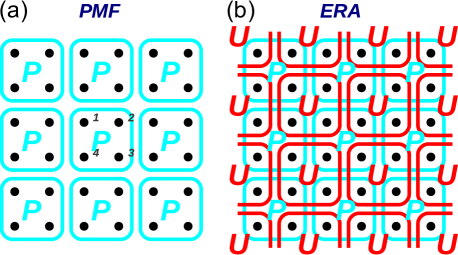
Figure 1: (color online). Two variational ansätze used in the present paper: (a) PMF, and (b) ERA. Black dots are lattice sites, ${\cal P}$’s are variational wave functions on $2\times 2$ plaquettes, and ${\cal U}$’s are variational $2\times 2$ unitary disentanglers.

Variational approach.— We begin with presenting two general variational methods for spin-orbital systems: (i) the plaquette MF (PMF) ansatz, see Fig. 1(a), and (ii) the entanglement renormalization ansatz (ERA) ERA , see Fig. 1(b). In the PMF, adapted here from a similar method for the bilayer KK model Brz11 , one employs a variational ansatz in a form of a product of plaquette $2\times 2$ wave functions ${\cal P}$’s plaq . Energy is minimized with respect to ${\cal P}$’s to obtain the best approximation to the ground state. ERA is a refined version of the PMF, where the product of ${\cal P}$’s is subject to an additional unitary transformation, being a product of $2\times 2$ “disentanglers” ${\cal U}$. They introduce entanglement between different plaquettes and make ERA more accurate.

Kugel-Khomskii model and methods.— The perturbation theory for a Mott insulator with active $e_{g}$ orbitals in the regime of $t\ll U$ leads to the spin-orbital model Ole00 , with the Heisenberg SU(2) spin interactions coupled to the orbital operators for the holes in the $d^{9}$ ionic states,

$${\cal H} = -\frac{1}{2}J\sum_{\langle ij\rangle||\gamma}\left\{\left(r_{1}\,\Pi_{t}^{(ij)}+r_{2}\,\Pi_{s}^{(ij)}\right)\left(\frac{1}{4}-\tau_{i}^{\gamma}\tau_{j}^{\gamma}\right)\right.$$ (1)

$$+ \left.\left(r_{3}+r_{4}\right)\Pi_{s}^{(ij)}\left(\frac{1}{2}-\tau_{i}^{\gamma}\right)\left(\frac{1}{2}-\tau_{j}^{\gamma}\right)\right\}+{\cal H}_{0}\,,$$

Each bond $\langle ij\rangle$ connects NN sites $\{i,j\}$ along one of the orthogonal axes $\gamma=a,b$ in the $ab$ plane. The model describes the spin-orbital superexchange in K₂CuF₄ Mos04 , with the superexchange constant $J=4t^{2}/U$. The coefficients $r_{1}\equiv 1/(1-3\eta)$, $r_{2}=r_{3}\equiv 1/(1-\eta)$, $r_{4}\equiv 1/(1+\eta)$ refer to the $d_{i}^{9}d_{j}^{9}\rightleftharpoons d_{i}^{8}d_{j}^{10}$ charge excitations to the upper Hubbard band Ole00 and depend on Hund’s exchange parameter

$$\eta=\frac{J_{H}}{U}.$$ (2)

The spin projection operators $\Pi_{ij}^{s}$ and $\Pi_{ij}^{t}$ select a singlet ($\Pi_{ij}^{s}$) or triplet ($\Pi_{ij}^{t}$) configuration for spins $S=1/2$ on the bond $\langle ij\rangle$, respectively,

$$\Pi_{s}^{(ij)}=\left(\frac{1}{4}-{\bf S}_{i}\cdot{\bf S}_{j}\right),\hskip 14.22636pt\Pi_{t}^{(ij)}=\left(\frac{3}{4}+{\bf S}_{i}\cdot{\bf S}_{j}\right).$$ (3)

Here $\tau_{i}^{\gamma}$ act in the subspace of $e_{g}$ orbitals occupied by a hole $\{|x\rangle,|z\rangle\}$, with $|z\rangle\equiv(3z^{2}-r^{2})/\sqrt{6}$ and $|x\rangle\equiv(x^{2}-y^{2})/\sqrt{2}$ — they can be expressed in terms of Pauli matrices $\{\sigma_{i}^{x},\sigma_{i}^{z}\}$ in the following way Ole00 :

$$\tau_{i}^{a(b)}\equiv\frac{1}{4}\left(-\sigma_{i}^{z}\pm\sqrt{3}\sigma_{i}^{x}\right),\quad\tau_{i}^{c}=\frac{1}{2}\,\sigma_{i}^{z}.$$ (4)

The term ${\cal H}_{0}$ in Eq. (1) is the crystal field splitting of two $e_{g}$ orbitals induced by the lattice geometry or pressure,

$${\cal H}_{0}=-E_{z}\sum_{i}\tau_{i}^{c}.$$ (5)

When $|E_{z}|\gg J$ it dictates the FO order with either $z$ or $x$ orbitals as long as we stay in the AF regime. This ground state can be further improved using perturbation theory in a dimensionless parameter $|\varepsilon_{z}|^{-1}\equiv J/|E_{z}|$.

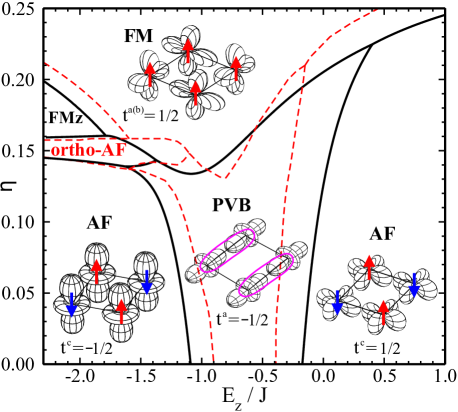
Figure 2: (color online). Phase diagram of the 2D KK model in the PMF (solid lines) and ERA (dashed lines) variational approximation. Insets show representative spin and orbital configurations on a $2\times 2$ plaquette — $x$-like ($t^{c}\!=\!\frac{1}{2}$) and $z$-like ($t^{a,c}\!=\!-\frac{1}{2}$) orbitals t_vals are accompanied either by AF spin order (arrows) or by spin singlets in the PVB phase (ovals). The FM phase has a two-sublattice AO order (with $t^{a(b)}\!=\!\frac{1}{2}$ at $E_{z}=0$) or FO$z$ order (FM$z$). In between the AF and FM (FM$z$) phase on finds an exotic ortho-AF phase — it has a noncollinear spin order, see text.

In the PMF one finds self-consistently MFs: $s_{i}^{\alpha}\equiv\langle S_{i}^{\alpha}\rangle$, $t_{i}^{\gamma}\equiv\langle\tau_{i}^{\gamma}\rangle$, and $v_{i}^{\alpha,\gamma}\equiv\langle S_{i}^{\alpha}\tau_{i}^{\gamma}\rangle$. Here $\gamma=a,b$, $\alpha=x,z$, and $i=1,\cdots,4$ labels sites of a single plaquette, see Fig. 1(a). We assume that either all plaquettes are the same, or that the neighboring plaquettes are rotated by $\pi/2$ with respect to each other in the $ab$ plane. In the latter case the order parameters are interchanged ($a\leftrightarrow b$) between neighboring plaquettes and transform as: $\{t_{i}^{a(b)}\}\to\{t_{i}^{b(a)}\}$ and $\{v_{i}^{\alpha,a(b)}\}\to\{v_{i}^{\alpha,b(a)}\}$. In the ERA treatment we either assume that all ${\cal P}$’s and ${\cal U}$’s are the same, like in Fig. 1(b), or divide the plaquette lattices of ${\cal P}$’s and ${\cal U}$’s into four sublattices with four independent ${\cal P}$’s and ${\cal U}$’s. One finds that the energy found in the ERA, when optimized with respect to both ${\cal U}$ and ${\cal P}$, is typically $5...15\%$ lower than the one in the PMF.

Phase diagram.— The phase diagram in $(\varepsilon_{z},\eta)$ plane contains six phases, see Fig. 2. The same phases appear in both the PMF and ERA — this suggests that the phase diagram is complete. At large $\eta$ one finds two FM phases: either with alternating orbital (AO) order as observed in K₂CuF₄ Ish96 ; Ish98 or with FO$z$ order (FM$z$). At $E_{z}<-1.8J$ a second order transition occurs from the FM to the FM$z$ phase (all other transitions involve both spins and orbitals are first order) at $\varepsilon_{z}/r_{1}=-0.934$ $(0.837)$ in the PMF (ERA). In these phases $\Pi^{(ij)}_{t}=1$ and the Hamiltonian (1) reduces to the $e_{g}$ orbital model You07 or to the generalized compass model Cin10 , in transverse field $E_{z}$. At $E_{z}=0$ one finds AO order with $\langle\sigma^{x}\rangle\neq 0$, while finite $E_{z}$ induces transverse polarization $\langle\sigma^{z}\rangle\neq 0$.

The phase diagram includes also two AF phases. They have uniform FO order with $\langle\sigma^{z}\rangle>0$ for $E_{z}>0$ and $\langle\sigma^{z}\rangle<0$ for $E_{z}<0$. The spin interactions in two AF phases are nonequivalent and are much weaker for $E_{z}<0$ than for $E_{z}>0$ — this difference increases up to a factor of 9 for fully polarized orbitals Ez>0 . These two phases are separated by the plaquette valence bond (PVB) phase with pairs of parallel spin singlets, horizontal or vertical and alternating between NN plaquettes. Note that the PVB phase is an analog of spin liquid phases found before for the 3D KK model Fei97 and for the bilayer Brz11 .

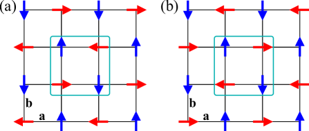
Figure 3: (color online). Schematic view of two nonequivalent spin configurations (a) and (b) of the classical ortho-AF phase $|\mathrm{AF}_{\perp}\rangle$ which cannot be transformed one into the other by lattice translations. Four spin directions (arrows) correspond to four spin sublattices — up/down arrows stand for eigenstates of $\left\langle S_{i}^{z}\right\rangle=\pm\frac{1}{2}$, while right/left arrows for $\left\langle S_{i}^{x}\right\rangle=\pm\frac{1}{2}$.

Finally, at $E_{z}<0$ and $\eta\sim 0.15$ we find a novel exotic "orthogonal AF" (“ortho-AF”) phase with entanglement ($v_{i}^{\alpha,\gamma}\neq 0$) which emerges in between the AF and the FM (FM$z$) phase. This state is characterized by the noncollinear magnetic order, see Fig. 3, with NN spins being orthogonal to each other and next-nearest neighbor (NNN) spins being AF. This phase is robust and has a somewhat extended range of stability in the ERA. In contrast to the frustrated spin $J_{1}$-$J_{2}$ interactions on a square lattice J1J2 , one finds here that $J_{1}$ is negligible and spin order follows from further neighbor couplings.

Effective spin model.— To explain the exotic magnetic order in the ortho-AF phase shown in Fig. 3 we derive an effective spin model for this phase. We show that NNN and third NN (3NN) spin interactions emerge here from the frustrated spin-orbital superexchange, ${\cal V}\equiv{\cal H}-{\cal H}_{0}$, treated as perturbation of the orbital ground state $|0\rangle$ of the unperturbed Hamiltonian ${\cal H}_{0}$ (5). Note an analogy to hidden multiple-spin interactions derived recently for frustrated Kondo lattice models Mot12 .

For negative $\varepsilon_{z}<0$ the ground state $|0\rangle$ of ${\cal H}_{0}$ is the FO$z$ state with $z$ orbitals occupied by a hole at each site, $\tau_{i}^{c}\left|0\right\rangle=-\frac{1}{2}\left|0\right\rangle$, and the energy $\varepsilon_{0}=-\frac{1}{2}|\varepsilon_{z}|$ per site. A finite gap that occurs for orbital excitations helps to remove high spin degeneracy in $|0\rangle$ by effective spin interactions in the Hamiltonian $H_{s}$ that can be constructed using the expansion in powers of $|\varepsilon_{z}|^{-1}$,

$$H_{s}\simeq J\left\{N\varepsilon_{0}+H_{s}^{(1)}+H_{s}^{(2)}+H_{s}^{(3)}\right\},$$ (6)

where $N$ is the number of sites. The first order term is an average $H_{s}^{(1)}\equiv\langle 0|{\cal V}|0\rangle$. Similarly, to evaluate $H_{s}^{(2)}$ and $H_{s}^{(3)}$ we determine the matrix elements $\langle n|{\cal V}|0\rangle$ for the excited states $|n\rangle$ with certain number of $z$-orbitals flipped to $x$-orbitals. All the averages are taken between orbital states and the spin model Eq. (6) follows.

The first order yields the Heisenberg Hamiltonian

$$H_{s}^{(1)}=\frac{1}{2^{5}}\left(-3r_{1}+4r_{2}+r_{4}\right)\sum_{\left\langle ij\right\rangle}\left({\bf S}_{i}\cdot{\bf S}_{j}\right).$$ (7)

The NN interaction $J_{1}\equiv(-3r_{1}+4r_{2}+r_{4})J/2^{5}$ changes sign at $\eta_{0}\simeq 0.155$ implying a direct AF-FM transition. However, this turns out to be a premature conclusion because the vanishing of $H_{s}^{(1)}$ at $\eta_{0}$ makes higher order terms in Eq. (6) relevant. Indeed, $\eta_{0}$ nicely falls into the ortho-AF area of the phase diagram in Fig. 2, where the NN interaction $J_{1}$ is small and frustrated.

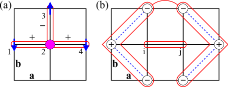
Figure 4: (color online). Artist’s views of the effective spin interactions obtained in: (a) second order $H_{s}^{(2)}$, with NNN term (123) and 3NN term (124), and (b) third order $H_{s}^{(3)}$. The frames in (a) indicate Heisenberg bonds multiplied along $a$ or $b$ axes with $\pm$ sign depending on the bond direction; the dot in the center stands for an orbital flip in $\left|0\right\rangle$. In (b) the dashed lines symbolize sums of three spins which enter each effective spin, ${\bf S}_{{\cal N}_{\gamma}(i)}$ and ${\bf S}_{{\cal N}_{\bar{\gamma}}(j)}$; the phase factors $s_{\gamma}$ (circles) and their scalar product are marked with connected frames.

Higher order terms.— Higher order terms arise by flipping orbitals from the ground state $|0\rangle$. Given that ${\cal V}$ has non-zero overlap only with states having one or two NN orbitals flipped from $z$ to $x$, one finds in second order,

$$H_{s}^{(2)}=\frac{\xi(\eta)}{|\varepsilon_{z}|}\left\{\sum_{\left\langle\left\langle ij\right\rangle\right\rangle}\!\left({\bf S}_{i}\cdot{\bf S}_{j}\right)-\tfrac{1}{2}\!\sum_{\left\langle\left\langle\left\langle ij\right\rangle\right\rangle\right\rangle}\!\left({\bf S}_{i}\cdot{\bf S}_{j}\right)\right\},$$ (8)

with $\xi(\eta)=(r_{1}+2r_{2}+3r_{4}){}^{2}/2^{10}$. Here $\langle\langle ij\rangle\rangle$ and $\langle\langle\langle ij\rangle\rangle\rangle$ stand for NNN and 3NN sites $i$ and $j$, see Fig. 4(a) for the origin and sign of these interactions. Apart from this, the second order also brings the $|\varepsilon_{z}|^{-1}$ correction to the Heisenberg interactions of $H_{s}^{(1)}$ (7), moving the transition point from $\eta_{0}$ to $\eta_{0}+O\left(\varepsilon_{z}^{-1}\right)$.

The NNN AF interaction in $H_{s}^{(2)}$ (8) alone would give two quantum antiferromagnets on interpenetrating sublattices spiral , but the additional 3NN FM term makes these AF states more classical than in the 2D Heisenberg model Suppl . This “double-AF” configuration is already similar to the ortho-AF phase in Fig. 3. However, the second order does not explain why the spins in the ortho-AF phase prefer to be orthogonal on NN bonds, and we have to proceed to the third order.

The third order in Eq. (6) produces many contributions to the spin Hamiltonian, but we are interested only in qualitatively new terms comparing to the lower orders. The terms bringing potentially new physics are the ones with connected products of three different Heisenberg bonds Suppl . The final result is a four-spin coupling,

$$H{}_{\perp}^{(3)}=\frac{1}{\varepsilon_{z}^{2}}\,\chi(\eta)\xi(\eta)\sum_{\langle ij\rangle||\gamma}\left({\bf S}_{i}\cdot{\bf S}_{j}\right)\left({\bf S}_{{\cal N}_{\gamma}(i)}\cdot{\bf S}_{{\cal N}_{\bar{\gamma}}(j)}\right),$$ (9)

where $\bar{\gamma}=-\gamma$ and ${\bf S}_{{\cal N}_{\gamma}(i)}\equiv\sum_{\alpha\not=\gamma}s_{\alpha}{\bf S}_{i+\alpha}$ is an effective spin around site $i$ in the direction $\gamma$, see Fig. 4(b). Here $\chi(\eta)=9(r_{1}+r_{4})/2^{7}$, $\alpha\in\{\pm a,\pm b\}$, and $s_{\alpha}=-1$ for $\alpha=\pm b$ and $s_{\alpha}=1$ otherwise. In the limit of two interpenetrating classical antiferromagnets $H_{\perp}^{(3)}$ gives the energy per site, $\varepsilon_{\perp}^{(3)}\approx\varepsilon_{z}^{-2}\chi(\eta)\xi(\eta)(\frac{3}{4}\cos\varphi)^{2}$, where $\varphi$ is an angle between the NN spins Suppl . This classical energy is minimized for $\varphi=\pi/2$ which explains the exotic magnetic order in the ortho-AF phase, shown in Fig. 3.

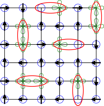
Figure 5: (color online). Artist’s view of the ortho-AF state $\left|\Psi_{\rm SO}\right\rangle$ (10), with spin order (arrows) of Fig. 3 and FO$z$ orbital order (circles) in the $ab$ plane. The state is dressed with spin singlets (ovals) entangled with either one or two orbital excitations from $|z\rangle$ to $|x\rangle$ orbitals (clovers) on NN bonds.

Spin-orbital entanglement.— The ground state $\left|\mathrm{AF}_{\perp}\right\rangle$ of $H_{s}$ (6) is nearly classical, except for small quantum corrections obtained within the spin-wave expansion Suppl . Thus one might expect that the spins are not entangled with orbitals. However, this argument overlooks that the resulting spins in $H_{s}$ are dressed with orbital and spin-orbital fluctuations. Indeed, within the perturbative treatment we obtain the full spin-orbital ground state,

$$\left|\Psi_{\rm SO}\right\rangle\propto\left(1-\sum_{n\not=0}\frac{{\cal V}_{n}}{\varepsilon_{n}}+\sum_{n,m\not=0}\frac{{\cal V}_{n}{\cal V}_{m}}{\varepsilon_{n}\varepsilon_{m}}-\dots\right)\left|\Phi_{0}\right\rangle,$$ (10)

where ${\cal V}_{n}\equiv\left|n\right\rangle\left\langle n\right|{\cal V}$, $\varepsilon_{n}$ are excitation energies, and $\left|\Phi_{0}\right\rangle\equiv|\mathrm{AF}_{\perp}\rangle|0\rangle$ is the disentangled classical state (Fig. 3). The operator sum in front of $\left|\Phi_{0}\right\rangle$ dresses this state with both orbital and spin-orbital fluctuations. When the purely orbital fluctuations are neglected and density of spin-orbital defects is assumed to be small, one finds

$$\left|\Psi_{\rm SO}\right\rangle\simeq\,\exp\left(-\frac{1}{|\varepsilon_{z}|}\sum_{\langle ij\rangle||\gamma}{\cal D}_{ij}^{\gamma}\right)\left|\Phi_{0}\right\rangle,$$ (11)

where

$${\cal D}_{ij}^{\gamma}=\left\{-A\,\sigma_{i}^{x}\sigma_{j}^{x}+B\left(\sigma_{i}^{x}+\sigma_{j}^{x}\right)s_{\gamma}\right\}\Pi_{ij}^{s}$$ (12)

is the spin-orbital excitation operator on the bond $\langle ij\rangle$, with $A=3(r_{1}+r_{4})/2^{6}$ and $B=\sqrt{3}(r_{1}+2r_{2}+3r_{4})/2^{5}$. Both terms in Eq. (12) project on a NN spin singlet, but the first one flips two NN $z$-orbitals while the second one generates only one flipped orbital. In short, the exponent $e^{-D/|\varepsilon_{z}|}$ dresses the classical ortho-AF state $|{\rm AF}_{\perp}\rangle$ in Fig. 3 with the entangled (spin-singlet/flipped-orbital) defects, see Fig. 5. The density of such entangled defects increases when $|\varepsilon_{z}|$ is decreased towards the PVB phase.

Topological defects.— The order parameter of the ortho-AF phase has non-trivial topology. The ground state is degenerate with respect to different orientations of its order parameter that consists of two orthogonal unit vectors defining orientation of each antiferromagnet. The first vector lives on the whole sphere $S^{2}$, but the second one is restricted to a circle $S^{1}$ because it is orthogonal to the first. In addition to spin-wave excitations, this $S^{2}\times S^{1}$ topology allows for skyrmions (textures) Wil83 and $\mathbb{Z}_{2}$-vortices (hedgehogs) as two types of topological defects. The hedgehog is stabilized by the orthogonality of the antiferromagnets. For instance, when one of them has fixed uniform orientation of its Néel order in space, the orthogonal orientation of the other one is free to make a hedgehog-like rotation.

Summary.— We have found surprising noncollinear spin order that arises from the NN spin-orbital superexchange when ferromagnetic and antiferromagnetic interactions almost compensate each other in the 2D KK model away from orbital degeneracy. It is stabilized by further neighbor spin exchange generated by entangled spin-orbital fluctuations which involve spin singlets and orbital flips. Similar mechanism works in the 3D KK model where it leads to a rich variety of spin-orbital phases to be reported elsewhere.

Finally, we note that magnetic order in spin-orbital systems may be changed by applying pressure Goode — indeed a transition from ferromagnetic to antiferromagnetic order was observed in K₂CuF₄ Ish96 ; Ish98 . Such a transition is also found here for a realistic value of $\eta\simeq 0.15$, and one could induce it in the antiferromagnetic phase by external magnetic field. Whether the antiferromagnetic order could be noncollinear as predicted here remains an experimental challenge.

Acknowledgments.— We thank G. Khaliullin, R. Kremer and B. Normand for insightful discussions. This work was supported by the Polish National Science Center (NCN) under Projects No. N202 069639 (W.B. and A.M.O.) and 2011/01/B/ST3/00512 (J.D.).

Supplemental Material

This supplement presents the technical details of the analysis employed in the paper. We first consider the third order terms in the perturbative expansion in section A. They justify the angle $\varphi=\pi/2$ obtained for the nearest neighbor (NN) spins in the regime of the noncollinear orthogonal antiferromagnetic (ortho-AF) phase. In section B we develop the spin-wave theory for the ortho-AF phase and calculate the quantum corrections to the order parameter. These calculations show that the noncollinear ortho-AF phase is stable with respect to the Gaussian fluctuations and the quantum corrections are here weaker than for the two-dimensional (2D) AF Heisenberg model.

.1 Third order terms in the perturbative expansion

The second order in the perturbation theory in $|\varepsilon_{z}|^{-1}$ results in two antiferromagnets on interpenetrating sublattices, but the angle $\varphi$ between the nearest neighbor (NN) spins remains undetermined, see Fig. 6(a). Thus we have to consider third order contributions to the effective spin Hamiltonian $H_{s}$ of the form:

$$H^{(3)}_{s}\! = \!\frac{1}{\varepsilon_{z}^{2}}\sum_{i,\gamma^{\prime}}s_{\gamma^{\prime}}\left[-J^{xz}\!(\eta){\bf S}_{i}\cdot{\bf S}_{i+\gamma^{\prime}}+K^{xz}\!(\eta)\right]$$ (13)

$$\times \!\sum_{\gamma\not=\gamma^{\prime}}\left[J^{xx}\!(\eta){\bf S}_{i}\cdot{\bf S}_{i+\gamma}\!+K^{xx}\!(\eta)\right]$$

$$\times \!\sum_{\gamma^{\prime\prime}\not=-\gamma}s_{\gamma^{\prime\prime}}\left[-J^{xz}\!(\eta){\bf S}_{i+\gamma}\cdot{\bf S}_{i+\gamma+\gamma^{\prime\prime}}\!+K^{xz}\!(\eta)\right]$$

$$+ \!\frac{1}{2\varepsilon_{z}^{2}}\sum_{i,\gamma}\left[J^{xx}(\eta){\bf S}_{i}\cdot{\bf S}_{i+\gamma}\!+K^{xx}\!(\eta)\right]$$

$$\times \!\sum_{\gamma^{\prime}\not=\gamma}s_{\gamma^{\prime}}\left[-J^{xz}(\eta){\bf S}_{i}\cdot{\bf S}_{i+\gamma^{\prime}}+K^{xz}\!(\eta)\right]$$

$$\times \!\!\sum_{\gamma^{\prime\prime}\not=-\gamma}\!s_{\gamma^{\prime\prime}}\left[-J^{xz}\!(\eta){\bf S}_{i+\gamma}\cdot{\bf S}_{i+\gamma+\gamma^{\prime\prime}}\!+K^{xz}\!(\eta)\right],$$

where: $J^{xz}(\eta)=2^{-5}\sqrt{3}\left(r_{1}\!+2r_{2}\!+3r_{4}\right)$, $K^{xz}(\eta)=2^{-7}\sqrt{3}\left(2r_{2}\!-3r_{1}+\!3r_{4}\right)$, $J^{xx}(\eta)=2^{-5}3\left(r_{1}+r_{4}\right)$ and $K^{xx}(\eta)=2^{-7}3\left(3r_{1}-r_{4}\right)$. Here and in all other equations in this Section a sum over $\gamma$ means the sum over all directions in the square lattice, i.e., $\gamma=\pm a,\pm b$.

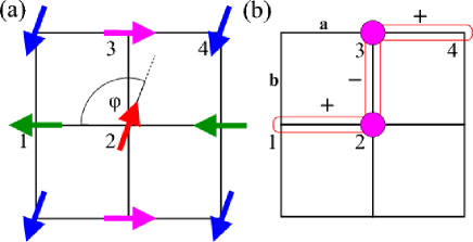
Figure 6: Panel (a): two independent AF orders realized by effective spin Hamiltonian $H_{s}$ up to second order. Angle $\varphi$ between the two neighboring spins is undetermined. Panel (b): exemplary third order correction to $H_{s}$ fixing the angle $\varphi$ as $\varphi=\pi/2$. Red frames stand for Heisenberg bond with $\pm$ sign depending on the bond’s direction and magenta dots indicate the single-site orbital excitations in the ground state.

The spin chains with less than three scalar products do not contribute with any qualitatively new terms. Once they are omitted we obtain:

$$H_{{\rm chain}}^{(3)}\! = \!\frac{9}{2^{16}\varepsilon_{z}^{2}}\left(r_{1}\!+\!r_{4}\right)\left(r_{1}\!+\!2r_{2}\!+\!3r_{4}\right)^{2}\sum_{i,\gamma}\sum_{{\gamma^{\prime}\not=\gamma\atop\gamma^{\prime\prime}\not=-\gamma}}$$

$$\!\left\{2s_{\gamma}s_{\gamma^{\prime\prime}}\left({\bf S}_{i+\gamma}\cdot{\bf S}_{i}\right)\left({\bf S}_{i}\cdot{\bf S}_{i+\gamma^{\prime}}\right)\!\left({\bf S}_{i+\gamma^{\prime}}\cdot{\bf S}_{i+\gamma^{\prime}+\gamma^{\prime\prime}}\right)\right.$$

$$+ \!s_{\gamma^{\prime}}s_{\gamma^{\prime\prime}}\left.\left({\bf S}_{i}\cdot{\bf S}_{i+\gamma}\right)\!\left({\bf S}_{i+\gamma^{\prime}}\cdot{\bf S}_{i}\right)\!\left({\bf S}_{i+\gamma}\cdot{\bf S}_{i+\gamma+\gamma^{\prime\prime}}\right)\right\},$$

where $s_{\gamma}$ is a sign factor depending on bond’s direction $\gamma$ originating from the definition of operators $\tau_{i}^{a,b}$ [see Fig. 6(b)], i.e.,

$$s_{\gamma}=\left\{\begin{array}[]{ccc}1&{\rm if}&\gamma=\pm a\\ -1&{\rm if}&\gamma=\pm b\end{array}\right..$$ (15)

We transform the second term of Eq. (LABEL:eq:3tild) using the vector identity:

$$\left({\bf S}_{i}\cdot{\bf S}_{i+\gamma}\right)\left({\bf S}_{i+\gamma^{\prime}}\cdot{\bf S}_{i}\right) =$$

$$\left({\bf S}_{i+\gamma^{\prime}}\cdot{\bf S}_{i}\right)\left({\bf S}_{i}\cdot{\bf S}_{i+\gamma}\right) + i{\bf S}_{i+\gamma}({\bf S}_{i+\gamma^{\prime}}\times{\bf S}_{i}).$$ (16)

The antihermitian term with a cross product cancels out under the sum in Eq. (LABEL:eq:3tild), thus we obtain:

$$H{}_{{\rm chain}}^{(3)}\! = \!\frac{9}{2^{16}\varepsilon_{z}^{2}}\left(r_{1}\!+\!r_{4}\right)\left(r_{1}\!+\!2r_{2}\!+\!3r_{4}\right)^{2}\sum_{i,\gamma}\sum_{{\gamma^{\prime}\not=\gamma\atop\gamma^{\prime\prime}\not=-\gamma}}$$

$$\!\left\{2s_{\gamma}s_{\gamma^{\prime\prime}}\!\left({\bf S}_{i+\gamma}\cdot{\bf S}_{i}\right)\!\left({\bf S}_{i}\cdot{\bf S}_{i+\gamma^{\prime}}\right)\left({\bf S}_{i+\gamma^{\prime}}\cdot{\bf S}_{i+\gamma^{\prime}+\gamma^{\prime\prime}}\right)\right.$$

$$+ \!s_{\gamma^{\prime}}s_{\gamma^{\prime\prime}}\left.\left({\bf S}_{i+\gamma^{\prime}}\cdot{\bf S}_{i}\right)\left({\bf S}_{i}\cdot{\bf S}_{i+\gamma}\right)\left({\bf S}_{i+\gamma}\cdot{\bf S}_{i+\gamma+\gamma^{\prime\prime}}\right)\right\}.$$

Now all the scalar products are ordered along the lines: $\left(i+\gamma\right)\to\left(i\right)\to\left(i+\gamma^{\prime}\right)\to\left(i+\gamma^{\prime}+\gamma^{\prime\prime}\right)$ and $\left(i+\gamma^{\prime}\right)\to\left(i\right)\to\left(i+\gamma\right)\to\left(i+\gamma+\gamma^{\prime\prime}\right)$. Next we use another spin identity, namely

$$\left({\bf S}_{1}\cdot{\bf S}_{2}\right)\left({\bf S}_{2}\cdot{\bf S}_{3}\right)\left({\bf S}_{3}\cdot{\bf S}_{4}\right)=$$

$$\frac{1}{16}\left({\bf S}_{1}\cdot{\bf S}_{4}\right)+\frac{1}{4}\left({\bf S}_{1}\cdot{\bf S}_{4}\right)\left({\bf S}_{2}\cdot{\bf S}_{3}\right)-\frac{1}{4}\left({\bf S}_{1}\cdot{\bf S}_{3}\right)\left({\bf S}_{2}\cdot{\bf S}_{4}\right)$$

$$+\frac{i}{8}\,{\bf S}_{1}\left({\bf S}_{3}\times{\bf S}_{4}\right)+\frac{i}{8}\,{\bf S}_{1}\left({\bf S}_{4}\times{\bf S}_{2}\right).$$ (18)

Again, the antihermitian cross-product terms cancel out under the sums in $H{}_{{\rm chain}}^{(3)}$.

To analyze the relevance of other terms in Eq. (18) we have to take into account that, to second order in the perturbation theory, there is nearly classical AF order on the two sublattices. We observe that:
(i) the first term is an AF interaction between the sublattices which is not compatible with the antiferromagnetism on the sublattices that is ${\cal O}(E_{z})$ stronger,
(ii) depending on its sign the second term may favour orthogonality of the two AF orders which is compatible with the order on sublattices, and
(iii) the third term brings no new information about the order.
Taking into account all three above arguments we argue that the relevant type-(ii) third order perturbative contributions of the form given by Eq. (18) may favour orthogonality of the two AF orders. Now we have to extract all such contributions from Eq. (18) and check if their overall sign is indeed positive.

After transforming Eq. (LABEL:eq:3tild2) we obtain

$$H_{\perp}^{(3)} = \frac{9}{2^{18}\varepsilon_{z}^{2}}\left(r_{1}\!+\!r_{4}\right)\left(r_{1}\!+\!2r_{2}\!+\!4r_{4}\right)^{2}\sum_{i,\gamma}\sum_{{\gamma^{\prime}\not=\gamma\atop\gamma^{\prime\prime}\not=-\gamma}}$$ (19)

$$\left[2s_{\gamma}s_{\gamma^{\prime\prime}}\!\left({\bf S}_{i+\gamma}\cdot{\bf S}_{i+\gamma^{\prime}+\gamma^{\prime\prime}}\right)\left({\bf S}_{i}\cdot{\bf S}_{i+\gamma^{\prime}}\right)\right.$$

$$+ s_{\gamma^{\prime}}s_{\gamma^{\prime\prime}}\left.\left({\bf S}_{i+\gamma^{\prime}}\cdot{\bf S}_{i+\gamma+\gamma^{\prime\prime}}\right)\!\left({\bf S}_{i}\cdot{\bf S}_{i+\gamma}\right)\right],$$

or in a more compact form

$$H_{\perp}^{(3)} = \frac{27}{2^{18}\varepsilon_{z}^{2}}\left(r_{1}\!+\!r_{4}\right)\left(r_{1}\!+\!2r_{2}\!+\!4r_{4}\right)^{2}\sum_{i,\gamma}\left({\bf S}_{i\cdot}{\bf S}_{i+\gamma}\right)$$ (20)

$$\times \left(\sum_{\gamma^{\prime}\not=\gamma}s_{\gamma^{\prime}}{\bf S}_{i+\gamma^{\prime}}\right)\!\!\cdot\!\!\left(\sum_{\gamma^{\prime\prime}\not=-\gamma}s_{\gamma^{\prime\prime}}{\bf S}_{i+\gamma+\gamma^{\prime\prime}}\right).$$

For two interpenetrating classical antiferromagnets $H_{\perp}^{(3)}$ gives the energy per site,

$$\varepsilon_{\perp}^{(3)}\approx\frac{1}{\varepsilon_{z}^{2}}\chi(\eta)\xi(\eta)\left(\frac{3}{4}\cos\varphi\right)^{2}\leavevmode\nobreak\ .$$ (21)

This classical energy is minimized for $\varphi=\pi/2$, i.e., when the NN spins on the bonds are orhogonal. This completes the argument that the orders in the two antiferromagnets prefer to be orthogonal.

.2 Spin wave expansion in the noncollinear ortho-AF phase

We start from the general form of the effective spin Hamiltonian:

$$H_{s} = \!A\sum_{\langle ij\rangle}{\bf S}_{i}\cdot{\bf S}_{j}+2B\!\sum_{\langle\langle ij\rangle\rangle}\!{\bf S}_{i}\cdot{\bf S}_{j}-B\!\sum_{\langle\langle\langle ij\rangle\rangle\rangle}\!{\bf S}_{i}\cdot{\bf S}_{j}$$

$$+ \!C\sum_{\langle ij\rangle||\gamma}\left({\bf S}_{i}\cdot{\bf S}_{j}\right)\!\!\sum_{{\gamma^{\prime}\not=\gamma\atop\gamma^{\prime\prime}\not=-\gamma}}\!s_{\gamma^{\prime}}s_{\gamma^{\prime\prime}}\left({\bf S}_{i+\gamma^{\prime}}\cdot{\bf S}_{i+\gamma+\gamma^{\prime\prime}}\right),$$

with coeffcients $A$, $B$ and $C$ being the functions of $\eta$ and $\varepsilon_{z}$, i.e.,

$$A = \frac{1}{2^{5}}\left(-3r_{1}+4r_{2}+r_{4}\right)$$ (23)

$$+ \frac{1}{\varepsilon_{z}}\frac{3}{2^{11}}\left\{3\left(r_{1}^{2}-r_{4}^{2}\right)-2\left(r_{1}+2r_{2}+3r_{4}\right)^{2}\right\},$$

$$B = -\frac{1}{\varepsilon_{z}}\frac{3}{2^{11}}\!\left(r_{1}+2r_{2}\!+3r_{4}\right){}^{\!2},$$ (24)

$$C = \frac{27}{2^{17}\varepsilon_{z}^{2}}\left(r_{1}+r_{4}\right)\left(r_{1}+2r_{2}+3r_{4}\right)^{2}.$$ (25)

To describe the ortho-AF order we divide the lattice into four sublattices as follows

$${\bf S}_{i,j}^{pq}\equiv{\bf S}_{p+2i,q+2j},\quad p,q\in\left\{1,2\right\},$$ (26)

where $p$ and $q$ form the sublattice label. In what follows all the sums over $p$ and $q$ run over the set $\{1,2\}$. Now, in each sublattice we do the linearized Holstein-Primakoff transformation around the ortho-AF order, i.e.,

$$\begin{array}[]{cccccc}S_{i,j}^{x,11}\!\!&\mathbf{=}\!\!&\frac{1}{2}\!\!\left(a_{i,j}^{11\dagger}+a_{i,j}^{11}\right),&S_{i,j}^{x,22}&\!\!\mathbf{=}\!\!&\frac{1}{2}\left(a_{i,j}^{22\dagger}+a_{i,j}^{22}\right),\\ S_{i,j}^{y,11}\!\!&\mathbf{=}\!\!&\frac{1}{2i}\!\!\left(a_{i,j}^{11}-a_{i,j}^{11\dagger}\right),&S_{i,j}^{y,22}&\!\!\mathbf{=}\!\!&\frac{1}{2i}\left(a_{i,j}^{22\dagger}-a_{i,j}^{22}\right),\\ S_{i,j}^{z,11}\!\!&\mathbf{=}\!\!&\left(\frac{1}{2}-a_{i,j}^{11\dagger}a_{i,j}^{11}\right),&S_{i,j}^{z,22}&\!\!\mathbf{=}\!\!&\left(a_{i,j}^{22\dagger}a_{i,j}^{22}-\frac{1}{2}\right),\end{array}$$ (27)

and

$$\begin{array}[]{cccccc}S_{i,j}^{x,12}\!\!&\mathbf{=}&\!\!\left(a_{i,j}^{12\dagger}a_{i,j}^{12}-\frac{1}{2}\right),&S_{i,j}^{x,21}&\!\!\mathbf{=}\!\!&\left(\frac{1}{2}-a_{i,j}^{21\dagger}a_{i,j}^{21}\right),\\ S_{i,j}^{y,12}\!\!&\mathbf{=}&\!\!\frac{1}{2}\!\!\left(a_{i,j}^{12\dagger}+a_{i,j}^{12}\right),&S_{i,j}^{y,21}&\!\!\mathbf{=}\!\!&\frac{1}{2}\!\!\left(a_{i,j}^{21\dagger}+a_{i,j}^{21}\right),\\ S_{i,j}^{z,12}\!\!&\mathbf{=}&\!\!\frac{1}{2i}\!\!\left(a_{i,j}^{12\dagger}-a_{i,j}^{12}\right),&S_{i,j}^{z,21}&\!\!\mathbf{=}\!\!&\frac{1}{2i}\!\!\left(a_{i,j}^{21}-a_{i,j}^{21\dagger}\right).\end{array}$$ (28)

Next step is the Fourier transform (FT):

$$a_{ij}^{pq}=\sum_{{\bf k}}e^{i(ik_{b}+jk_{a})}a_{{\bf k}}^{pq},$$ (29)

followed by the phase transformation, in order to get rid of imaginary parts in $H_{s}$ of Eq. (.2) after FT,

$$a_{{\bf k}}^{11\dagger}\to a_{{\bf k}}^{11\dagger}e^{-i\frac{k_{a}}{2}}, a_{{\bf k}}^{12}\to ia_{k}^{12},$$

$$a_{{\bf k}}^{21}\to-ia_{{\bf k}}^{21}e^{i\frac{k_{a}}{2}}e^{-i\frac{k_{b}}{2}}, a_{{\bf k}}^{22\dagger}\to a_{{\bf k}}^{22\dagger}e^{i\frac{k_{b}}{2}}.$$ (30)

Finally, the interactions in the $H_{s}$ Hamiltonian take the following form:

$$\sum_{\left\langle ij\right\rangle}\!{\bf S}_{i}\cdot{\bf S}_{j}\! = \!\frac{1}{2}\!\sum_{{\bf k}}\cos\frac{k{}_{b}}{2}\left(a_{-{\bf k}}^{21\dagger}\!-a_{{\bf k}}^{21}\right)\left(a_{{\bf k}}^{11\dagger}\!-a_{-{\bf k}}^{11}\right)$$

$$+ \!\frac{1}{2}\!\sum_{{\bf k}}\cos\frac{k{}_{b}}{2}\!\!\left(a_{-{\bf k}}^{12\dagger}\!-a_{{\bf k}}^{12}\right)\left(a_{{\bf k}}^{22\dagger}\!-a_{-{\bf k}}^{22}\right)$$

$$- \!\frac{1}{2}\!\sum_{{\bf k}}\cos\frac{k{}_{a}}{2}\!\!\left(a_{-{\bf k}}^{12\dagger}\!-a_{{\bf k}}^{12}\right)\left(a_{{\bf k}}^{11\dagger}\!-a_{-{\bf k}}^{11}\right)$$

$$- \!\frac{1}{2}\!\sum_{{\bf k}}\cos\frac{k{}_{a}}{2}\!\left(a_{-{\bf k}}^{21\dagger}\!-a_{{\bf k}}^{21}\right)\left(a_{{\bf k}}^{22\dagger}\!-a_{-{\bf k}}^{22}\right),$$

for the NN interactions,

$$\sum_{\langle\langle ij\rangle\rangle}\!{\bf S}_{i}\cdot{\bf S}_{j}\! = 2\sum_{{\bf k}}\left\{\gamma^{\prime}_{{\bf k}}\left(a_{{\bf k}}^{11\dagger}a{}_{-{\bf k}}^{22\dagger}+a_{{\bf k}}^{12\dagger}a_{-{\bf k}}^{21\dagger}\right)+H.c.\right\}$$ (32)

$$+ 2\sum_{{\bf k}}\sum_{p,q}a_{{\bf k}}^{pq\dagger}a_{{\bf k}}^{pq},$$

for the NNN interactions,

$$\sum_{\left\langle\left\langle\left\langle i,j\right\rangle\right\rangle\right\rangle}{\bf S}_{i}\cdot{\bf S}_{j}=2\sum_{{\bf k}}\sum_{p,q}a_{{\bf k}}^{pq\dagger}a_{{\bf k}}^{pq}\left(\gamma_{{\bf k}}-1\right)$$ (33)

for the 3NN interactions, and

$$\sum_{i,\gamma}\left({\bf S}_{i}\cdot{\bf S}_{i+\gamma}\right)s_{\gamma^{\prime}}s_{\gamma^{\prime\prime}}\sum_{{\gamma^{\prime}\not=\gamma\atop\gamma^{\prime\prime}\not=-\gamma}}\left({\bf S}_{i+\gamma^{\prime}}\cdot{\bf S}_{i+\gamma+\gamma^{\prime\prime}}\right)=$$ (34)

$$12\sum_{\bf k}\sum_{p,q}\gamma_{\bf k}\left(a_{\bf k}^{pq\dagger}+a_{-\bf k}^{pq}\right)\left(a_{-\bf k}^{pq\dagger}+a_{\bf k}^{pq}\right)$$

$$- 48\sum_{\bf k}\gamma^{\prime}_{k}\left(a_{\bf k}^{12\dagger}+a_{-\bf k}^{12}\right)\left(a_{-\bf k}^{21\dagger}+a_{\bf k}^{21}\right)$$

$$- 48\sum_{\bf k}\gamma^{\prime}_{\bf k}\left(a_{\bf k}^{11\dagger}+a_{-\bf k}^{11}\right)\left(a_{-\bf k}^{22\dagger}+a_{\bf k}^{22}\right)$$

$$+ 36\sum_{\bf k}\left(a_{\bf k}^{11\dagger}+a_{-\bf k}^{11}\right)\left(a_{-\bf k}^{21\dagger}+a_{\bf k}^{21}\right)\cos\frac{k_{b}}{2}$$

$$+ 36\sum_{\bf k}\left(a_{\bf k}^{12\dagger}+a_{-\bf k}^{12}\right)\left(a_{-\bf k}^{22\dagger}+a_{\bf k}^{22}\right)\cos\frac{k_{b}}{2}$$

$$- 36\sum_{\bf k}\left(a_{\bf k}^{11\dagger}+a_{-\bf k}^{11}\right)\left(a_{-\bf k}^{12\dagger}+a_{\bf k}^{12}\right)\cos\frac{k_{a}}{2}$$

$$- 36\sum_{\bf k}\left(a_{-\bf k}^{21\dagger}+a_{\bf k}^{21}\right)\left(a_{\bf k}^{22\dagger}+a_{-\bf k}^{22}\right)\cos\frac{k_{a}}{2},$$

for the third order interactions between the two AF sublattices. The coefficients $\{\gamma_{\bf k},\gamma^{\prime}_{\bf k}\}$ are defined as:

$$\gamma_{\bf k} \equiv \frac{1}{2}\left(\cos k{}_{b}+\cos k{}_{a}\right),$$ (35)

$$\gamma^{\prime}_{\bf k} \equiv \frac{1}{2}\left(\cos\frac{k_{a}+k_{b}}{2}+\cos\frac{k_{a}-k_{b}}{2}\right).$$ (36)

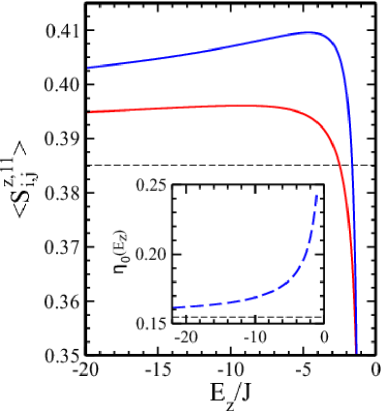
Figure 7: The sublattice magnetization $\left\langle S_{i,j}^{z,11}\right\rangle$ as function of $\varepsilon_{z}$ in the ortho-AF phase for: $\eta_{0}$ constant such that $A\left(\eta_{0}\right)=0$ for $\varepsilon_{z}\to-\infty$ (lower-red curve), and $\eta_{0}\left(\varepsilon_{z}\right)$ such that $A\left(\eta_{0}\right)=0$ for any $\varepsilon_{z}$ (upper-blue curve). The inset shows the function $\eta_{0}(E_{z})$ with its asymptote for $\varepsilon_{z}\to-\infty$ marked with the black dashed line.

The last step is the Bogoliubov transformation of the block-diagonal Hamiltonian $H_{s}$ in the momentum space. The most general form of this transformation is:

$$\left(\begin{array}[]{c}\bm{b}_{\bf k}^{\dagger}\\ \bm{b}_{-\bf k}\end{array}\right)=\bm{{\cal B}}_{\bf k}\!\left(\begin{array}[]{c}\bm{a}_{\bf k}^{\dagger}\\ \bm{a}_{-\bf k}\end{array}\right).$$ (37)

Here $\bm{b}_{\bf k}^{\dagger}\equiv\{b_{\bf k}^{pq\dagger}\}$ are the new boson operators and $\bm{{\cal B}}_{\bf k}$ is an $8\times 8$ transformation matrix to be determined from the Bogoliubov-de Gennes eigenequation,

$$[H_{s},b_{\bf k}^{pq\dagger}]=E_{\bf k}^{pq}\,b_{\bf k}^{pq\dagger},$$ (38)

equivalent to an $8\times 8$ matrix eigenproblem with hyperbolic normalization conditions typical for bosons. The resulting eigen-vectors form the rows $\bm{{\cal B}}_{\bf k}$ and the excitation energies $E_{\bf k}^{pq}$ can be expressed analytically as,

$$\left(E_{\bf k}^{pq}\right)^{2} = 2^{4}\left(1-\gamma_{\bf k}^{pq}\right)\left\{B-6C+\left(B-24C\right)\gamma_{\bf k}^{pq}\right\}$$

$$\times \left\{3B+A\gamma_{\bf k}^{pq}-B\left(\gamma_{\bf k}-2\left(-1\right){}^{p+q}\gamma^{\prime}_{\bf k}\right)\right\},$$

with

$$\gamma_{\bf k}^{pq}=\frac{1}{2}\left\{\left(-1\right)^{p}\cos\frac{k_{a}}{2}+\left(-1\right)^{q}\cos\frac{k_{b}}{2}\right\}.$$ (40)

As might have been expected, in addition to the three gapless Goldstone modes for $\left(p,q\right)=\left(2,2\right),\left(1,2\right),\left(2,1\right)$, there is one gapped branch $E_{\bf k}^{11}$, with $E_{\bf k=0}^{11}=24\sqrt{\left(4B-A\right)C}$, related to the rigidity of the angle $\varphi$ between the two antiferromagnets.

Another important quantity is the magnetization on a sublattice which quantifies quantum fluctuations. For instance, the ground state expectation value of $S_{i,j}^{z,11}$ can be expressed by the elements of $\bm{{\cal B}}_{\bf k}^{-1}$,

$$\left\langle S_{i,j}^{z,11}\right\rangle=\frac{1}{2}-\frac{1}{4\pi^{2}}\intop_{-\pi}^{\pi}\sum_{p=5}^{8}\left\{\bm{{\cal B}}_{\bf k}^{-1}\right\}_{1,p}^{2}d^{2}k.$$ (41)

The integrand in the above formula can be obtained analytically whereas the integration is non-algebraic. In Figs. 7 and 8 we show the behavior of $\left\langle S_{i,j}^{z,11}\right\rangle$ along different cuts of the ortho-AF phase.

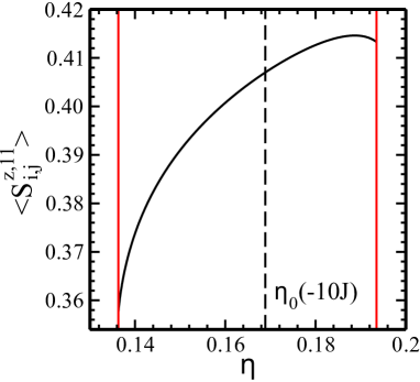
Figure 8: The sublattice magnetization $\left\langle S_{i,j}^{z,11}\right\rangle$ as function of $\eta$ in the ortho-AF phase for $\varepsilon_{z}=-10$ (solid line). Dashed line marks the value of $\eta_{0}$ where $A=0$. The vertical solid (red) lines are boundaries of the spin-wave expansion, where the integral (41) becomes divergent.

Both cuts in Fig. 7 take the same value of $\left\langle S_{i,j}^{z,11}\right\rangle\simeq 0.385$ in the limit of $\varepsilon_{z}\to-\infty$ when the coupling between the two antiferromagnets is negligible. This magnetization is markedly higher than that for the 2D AF Heisenberg model, where $\left\langle S^{z}\right\rangle\simeq 0.303$. This confirms that the NNN FM interactions in $H_{s}$ make the AF order more robust against quantum fluctuations. What is more, along the line $\eta_{0}(\varepsilon_{z})$ (blue curve) the third order term $\propto C$ enhances the order parameter up to $\left\langle S_{i,j}^{z,11}\right\rangle\simeq 0.405$ near $\varepsilon_{z}=-4$. Deviations from the path $\eta_{0}\left(\varepsilon_{z}\right)$ that introduce nonzero coefficient $A$ of the NN AF coupling can either impair or enhance the ortho-AF order. For instance, the red curve lies below the blue one in Fig. 7. In contrast, the cut along the line $\varepsilon_{z}=-10$ in Fig. 8 shows that a small increase of $\eta$ above $\eta_{0}$ can increase the magnetization (at this value of $\varepsilon_{z}$). This reflects the proximity to the ferromagnetic phase where the quantum fluctuations reducing the order parameter $\left\langle S_{i,j}^{z,11}\right\rangle$ are suppressed.

The sudden collapse of the blue and red curves in Fig. 7 terminates the ortho-AF phase in the spin wave approach. However, this is not a definitive conclusion because the perturbative Hamiltonian $H_{s}$ underlying the spin wave expansion is not self-consistent for $\varepsilon_{z}>-4$, where the third order term $\propto C$ in $H_{s}$ dominates over the second order term $\propto B$. In the non-perturbative plaquette MF the ortho-AF phase extends far beyond the perturbative regime, and it is even more extended in the more accurate ERA approach.