Iterative unfolding with the Richardson-Lucy algorithm

Abstract

The Richardson-Lucy unfolding approach is reviewed. It is extremely simple and excellently performing. It efficiently suppresses artificial high frequency contributions and permits to introduce known features of the true distribution. An algorithm to optimize the number of iterations has been developed and tested with five different types of distributions. The corresponding unfolding results were very satisfactory independent of the number of events, the number of bins in the observed and the unfolded distribution, and the experimental resolution.

1 Introduction

In many experiments the measurements are deformed by limited acceptance, sensitivity or resolution of the detectors. To be able to compare and combine results from different experiments and to compare the published data to a theory, the detector effects have to be unfolded. While acceptance losses can be corrected for, unfolding resolution effects is quite involved. Naive methods produce oscillations in the unfolded distribution that have to be suppressed by regularization schemes.

Various unfolding methods have been proposed in particle physics [1, 2, 3]. The data are usually treated in form of histograms. This is also the case in the Richardson-Lucy (R-L) method [4, 5] which is especially simple, reliable, independent of the dimension of the histogram and independent of the underlying metric.

Iterative unfolding with the R-L algorithm has initially been used for picture restoration. Shepp and Vardi [6, 7], and independently Kondor, [8] have introduced it into physics. It corresponds to a gradual unfolding. Starting with a first guess of the smooth true distribution, this distribution is modified in steps such that the difference between its smeared version and the observed distribution is reduced. With increasing number of steps, the iterative procedure develops oscillations. These are avoided by stopping the iterations as soon as the unfolded distribution, when folded again, is compatible with the observed data within the uncertainties. We will discuss the details below. The R-L algorithm originally was derived using Bayesian arguments [4] but it can also be interpreted in a purely mathematical way [9, 10]. It became finally popular in particle physics after it had been promoted by D’Agostini [11] with the label “Bayesian unfolding”. In Ref. [12] it was adapted to unbinned unfolding. In Ref. [13] the R-L algorithm was applied to a 4-dimensional distribution.

The present situation in particle physics is unsatisfactory for two reasons: i) There is a lack of comparative systematic studies of the different unfolding methods and ii) the way to fix the degree of smoothing, the regularization strength, is usually only vaguely defined.

In the following section we introduce the notation and formulate the mathematical relations. In Section 3 we discuss regularization and the problem of assigning errors to the unfolded distribution. In Section 4 the R-L iterative approach is described. A criterion is developed to fix the number of iterations that have to be applied and which determine the degree of regularization. Section 5 contains examples. We conclude with a summary and recommendations.

2 Definitions and basic relations

An event sample with variables $\{x_{1},\ldots,x_{n}\}$, the input sample is produced according to a statistical distribution $f(x)$. It is observed in a detector. The observed sample $\{x_{1}^{\prime},\ldots,x_{n^{\prime}}^{\prime}\}$ is distorted due the finite resolution of the detector and reduced because of acceptance losses. We distinguish between four different histograms: The true histogram with content $\theta_{j}$, $j=1,\ldots,N$ of bin $j$. $\theta_{j}\propto\int_{bin\text{ }j}f(x)dx$ corresponds to $f(x)$. The input histogram contains the input sample. The content of its bin $j$ is drawn from a Poisson distribution with mean value $\theta_{j}$. The observed histogram contains the observed sample with $d_{i}$ events in bin $i$, $i=1,\ldots,M$. The expected number of events $t_{i}$ in bin $i$ is given by $t_{i}\propto\int_{bin\text{ }i}f^{\prime}(x^{\prime})dx^{\prime}$ where  the functions $f^{\prime}$ and $f$ are related through $f^{\prime}(x^{\prime})=\int g(x^{\prime},x)f(x)dx$ with the response function $g(x^{\prime},x)$. We choose $M>N$  to constrain the problem. The result of the unfolding procedure is again a histogram, the unfolded histogram, with bin content $\hat{\theta}_{j}$. We are confronted with a standard inference problem where the wanted parameters are the bin contents $\theta_{j}$ of the true histogram. It is to be solved by a least square (LS) or a maximum likelihood (ML) fit. We discuss only one-dimensional histograms but the corresponding array may represent a multi-dimensional histogram with arbitrarily numbered cells as well.

The numbers $t_{i}$ and $\theta_{j}$ are related by the linear relation

$$t_{i}=\sum_{j=1}^{N}A_{ij}\theta_{j}$$ (1)

with the response matrix $A_{ij}$

$$A_{ij}=\frac{\int_{bin\text{ }i}f^{\prime}(x^{\prime})dx^{\prime}}{\int_{bin\text{ }j}f(x)dx}\;.\;$$

$A_{ij}$  is the probability to observe an event in bin $i$ that belongs to the true bin $j$. We calculate $A_{ij}$ by a Monte Carlo simulation, but as we do not know $f(x)$, we have to use a first guess of it. If the size of the bins is smaller than the experimental resolution, the elements of the response matrix show little dependence on the distribution that is used to generate the events.

We assume that the observed values $d_{i}$ fluctuate according to the Poisson distribution with the expectation $t_{i}$ and the variance $\delta_{i}^{2}=t_{i}$.

The representation of the unfolded distribution by a histogram is a first smoothing step. We call it implicit regularization. With wide enough bins, strong oscillations in the unfolded histogram are avoided. LS or ML fits will produce the parameter estimates $\hat{\theta}_{j}$ together with reliable error estimates. With the prediction $t_{i}$ for $d_{i}$ we can define $\chi^{2}$,

$$\chi^{2}={\displaystyle\sum\limits_{i=1}^{M}}\frac{\left[d_{i}-t_{i}\right]^{2}}{t_{i}}\;,$$ (2)

and the log-likelihood $\ln L$ derived from the Poisson distribution,

$$\ln L=\sum_{i=1}^{M}\left[d_{i}\ln t_{i}-t_{i}\right]\;.$$ (3)

Minimizing $\chi^{2}$ or maximizing $\ln L$ determines the estimates of the parameters $\hat{\theta}_{j}$. The ML fit is applicable also with small event numbers $d_{i}$ and suppresses negative estimates of the parameter values. Negative values can occur in rare cases.

3 The regularization and the error assignment

In particle physics the data are often distorted by resolution effects. This means that without regularization the number of events in neighboring bins of the unfolded histogram are negatively correlated and as a consequence local fluctuations are observed. More precisely, the fitted parameters $\hat{\theta}_{j},\hat{\theta}_{j^{\prime}}$ in two true bins $j,j^{\prime}$ are anti-correlated if their events have sizable probabilities $A_{ij},A_{ij^{\prime}}$ to fall into the same observed bin $i$. These specific correlations are taken into account in most unfolding methods. An exception is entropy regularization [14, 15, 16] which also penalizes fluctuations between distant bins.

The $\chi^{2}$ surface of the unregularized fit near its minimum $\chi_{0}^{2}$ is rather shallow and large correlated parameter changes produce only small changes $\Delta\chi^{2}$ of $\chi^{2}$ of the fit. The location of the true parameter point in the parameter space is badly known but the surfaces of $\chi_{0}^{2}+\Delta\chi^{2}$ for not too small values of $\Delta\chi^{2}$ are well defined and fix the error intervals which should not be affected by the regularization. We are allowed to move the point estimate but the error intervals should not be shifted. The regularization should lead only to a small increase of $\chi^{2}$. The increase $\Delta\chi^{2}=\chi^{2}-\chi_{0}^{2}$ defines an $N$ dimensional error interval around the fitted point in the parameter space. It can be converted to a $p$-value

$$p=\int_{\Delta\chi^{2}}^{\infty}u_{N}(z)dz$$ (4)

where $u_{N}$ is the $\chi^{2}$ distribution for $N$ degrees of freedom. Strictly speaking, $p$ is a proper $p$-value only in the limit where the test quantity $\chi^{2}$ is described by a $\chi^{2}$ distribution. Fixing $p$ fixes the regularization strength. A large value of $p$ corresponds to a weak regularization and means that the unfolding result is well inside the commonly used error interval of the likelihood fit. The optimal value of a cut in  $p$ depends on the unfolding method. Remark that here the value of $\chi_{0}^{2}$ of the fit is irrelevant; what is relevant is its change due to the regularization. A large value $\chi_{0}^{2}$ could indicate that something is wrong with the model.

In most applications outside physics, like picture restoration, the uncertainties of the unfolded distribution are of minor concern. Of interest are mainly the point estimates which are obtained with a regularization that the user chooses according to his personal experience. In physics problems, the error bounds are as important as the point estimates. The manipulations related to the regularization in most methods constrain the fit and therefore reduce the errors of the unfolded histogram as provided by the unconstrained fit [17, 18]. As a consequence, these errors depend on the regularization strength and do not cover the true distribution with a fixed probability. Distributions with narrow structures that are compatible with the data may be excluded. An example for such a behavior is presented in Appendix 1. It is not possible to associate classical confidence intervals to explicitly regularized solutions. As stated above, standard error intervals are provided by fits without regularization.

In the iterative method the errors could in principle be calculated by error propagation but these errors would not be constrained and therefore usually be large and strongly correlated. Furthermore their interpretation would be difficult. Therefore it does not make sense to include them in the graphical representation. A very qualitative way to indicate the errors is presented in Appendix 2.

To document quantitatively the precision of the data, a fit with a small number of bins and without explicit regularization of the unfolded histogram should be done, such that by a wide enough binning artificial oscillations are sufficiently suppressed. The result together with the corresponding error matrix estimate contain the information that is necessary for a comparison with theoretical predictions or other experiments. An example is given in Appendix 2. Alternatively, the data vector and the response matrix could be kept. These items, however, require some explanation to non-experts.

In case we have a theoretical prediction in analytic form, depending on unknown parameters, we should avoid unfolding and the regularization problem and estimate the parameters directly [19]. A direct fit does not require the construction of a response matrix and is independent of assumptions about the shape of the distribution used to simulate the experiment, parameter inference is possible even with very low event numbers where unfolding is problematic, the results are unbiased and the full information contained in the experimental data can be explored.

4 The Richardson-Lucy iteration

4.1 The method

Replacing the expected number $t_{i}$ in relation (1) by the observed number $d_{i}$, the corresponding matrix relation $d=A\hat{\theta}$ can be solved iteratively for the estimate $\hat{\theta}$. The idea behind the iteration algorithm is the following: Starting with a preliminary guess $\hat{\theta}^{(0)}$of $\theta$, the corresponding prediction for the observed distribution $d^{(0)}$ is computed. It is compared to $d$ and for a bin $i$ the ratio $d_{i}/d_{i}^{(0)}$ is formed which ideally should be equal to one. To improve the agreement, all true components are scaled proportional to their contribution $A_{ij}\hat{\theta}_{j}^{(0)}$ to $d_{i}^{(0)}$. This procedure when iterated corresponds to the following steps:

The prediction $d^{(k)}$ of the iteration $k$ is obtained in a folding step from the true vector $\hat{\theta}^{(k)}$:

$$d_{i}^{(k)}=\sum_{j=1}^{N}A_{ij}\hat{\theta}_{j}^{(k)}\;.$$ (5)

In an unfolding step, the components $A_{ij}\hat{\theta}_{j}^{(k)}$ are scaled with $d_{i}/d_{i}^{(k)}$ and added up into the bin $j$ of the true distribution from which they originated:

$$\hat{\theta}_{j}^{(k+1)}=\sum_{i=1}^{M}A_{ij}\hat{\theta}_{j}^{(k)}\frac{d_{i}}{d_{i}^{(k)}}\left/\alpha_{j}\right.\;.$$ (6)

Dividing by the acceptance $\alpha_{j}=\sum_{i}A_{ij}$ corrects for acceptance losses.

The result of the iteration converges to the maximum likelihood solution as was proven by Vardi et al. [7] and Mülthei and Schorr [9] for Poisson distributed bin entries. Since we start with a smooth initial distribution, the artifacts of the unregularized ML estimate (MLE) occur only after a certain number of iterations.

The regularization is performed simply by interrupting the iteration sequence. As explained above, the number of applied iterations should be based on a $p$-value criterion which measures the compatibility of the regularized unfolding solution with the MLE.

To this end, first the number of iterations is chosen large enough to approach the asymptotic limit with the ML solution which provides the best estimate of the true histogram if we put aside our prejudices about smoothness. Folding the result and comparing it to the observed histogram, we obtain $\chi_{0}^{2}$ of the fit.

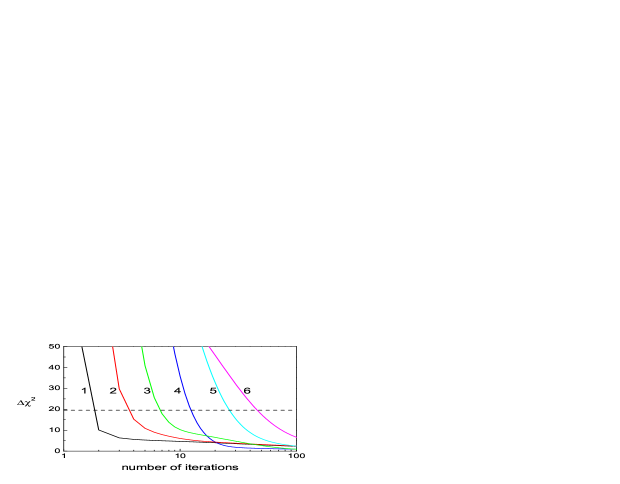
Figure 1: Convergence of the iterative unfolding for distributions with 1 to 6 oscillations.

Of course, the MLE does not depend on the starting distribution but the regularized solution obtained by stopping the iteration does. We may choose it according to our expectation. In most cases the detailed shape of it does not matter, and a uniform starting distribution will provide reasonable results.

As may be expected, the speed of convergence decreases with the spatial frequency of the true distribution if we consider a Gaussian type of smearing described by a point spread function. This is shown in Fig. 1. Here the true distributions consisting of a superposition of a uniform distribution of $1000$ events and a squared sine/cosine distributions of $9000$ events with $1$ to $6$ oscillations is smeared and distributed into $40$ bins. The corresponding histogram is unfolded to a $20$ bin histogram starting with a uniform histogram. The statistic $\Delta\chi^{2}$ for $20$ degrees of freedom is plotted as a function of the number of iterations. The discrete points are connected by a line. The horizontal line corresponds to a $p$-value of $0.5$. As expected, the number of required iteration steps that are needed to reach the $p=0.5$ value increases with the frequency of the distribution. This means that high frequency contributions and artificial fluctuations of correlated bins are strongly suppressed in the R-L approach. The reason can be inferred from Relation (6): The parameters $\theta_{j},\theta_{j^{\prime}}$ of bins $j,j^{\prime}$ that are correlated in that they have similar values $A_{ij}$, $A_{ij^{\prime}}$ are scaled in a similar way and relative fluctuations develop only slowly with increasing number of iterations.

Remark: By construction, the R-L method is invariant against an arbitrary re-ordering of the bins. A multidimensional histogram can be transformed to a one-dimensional histogram. A rather general class of distortions can be treated. This is also true for entropy regularization and methods based on truncation of the eigenvalue sequence in singular value decomposition (SVD) [17] but not for local regularization schemes like curvature suppression [20] which is difficult to apply in higher dimensions.

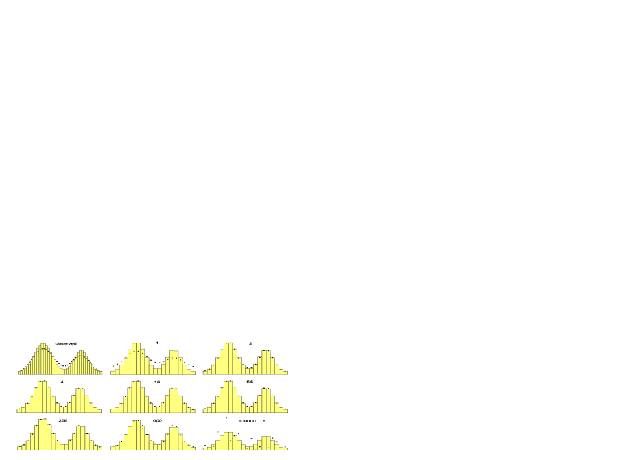
Figure 2: Observed histogram and unfolded histograms (squares) for different number of iterations compared to the input histogram (shaded).

4.2 The regularization strength

Without recipes how to fix the regularization strength, unfolding methods are incomplete and the results are to a certain extent arbitrary. In most of the proposed methods a recommendation is missing or rather vague. In the iterative method, we have to find a criterion, based on a $p$-value, when to stop the iteration process. The optimum way may depend on several parameters: the number of events, the number of bins, the resolution and the shape of the true distribution. Not all combinations of these parameters can be investigated in detail. We will study some specific Monte Carlo examples to derive a stopping criterion and then test it with further distributions. It will be shown that a general prescription works reasonably well for all studied examples.

The unfolded histogram is compared to the input histogram. In all examples we take care that the estimates of the elements of the response matrix have negligible statistical uncertainties. If not stated differently, the iteration starts with a uniform distribution as a first guess for the true distribution. The observed histogram has, with two exceptions, $40$ bins and the unfolded histogram usually comprises $20$ bins. With the standard settings the value of $\chi_{0}^{2}$ should be compatible with the $\chi^{2}$ distribution with $20$ degrees of freedom because we have $40$ measurements and $20$ estimated parameters.

Example 1: Two peaks

We start with a two-peak distribution, a superposition of two normal distributions $N(x|0.3;0.10)$, $N(x|0.75;0.08)$ and a uniform distribution $U(x)$ in the interval $0<x<1$. Here $N(x|\mu;\sigma$) is the normal distribution of $x$ with the mean value $\mu$ and the standard deviation $\sigma$. The number of events attributed to the three distributions is $25,000$, $15,000$ and $10,000$, respectively. The experimental distribution is observed with a Gaussian resolution $\sigma=0.07.$ It is of the same order as the width of the peaks. Events are accepted in the interval $0<x,x^{\prime}<1$.

In Fig. 2 unfolding results for different values of the number of iterations are shown. The shaded histograms (input histograms) correspond to the observation with an ideal detector and are close to the true histogram. The left top plot displays the observed histogram as squares. With increasing number of iterations the unfolded histogram (squares) quickly approaches the true histogram. The agreement is quite good in a wide range of the number of iterations. It deteriorates slowly when increasing the number of iterations beyond $32$. At $1000$ iterations oscillations are visible and after $100,000$ iterations the sequence has approached the maximum likelihood solution with strong fluctuations and no explicit regularization. We find $\chi_{0}^{2}=23.4$ for $20$ degrees of freedom.

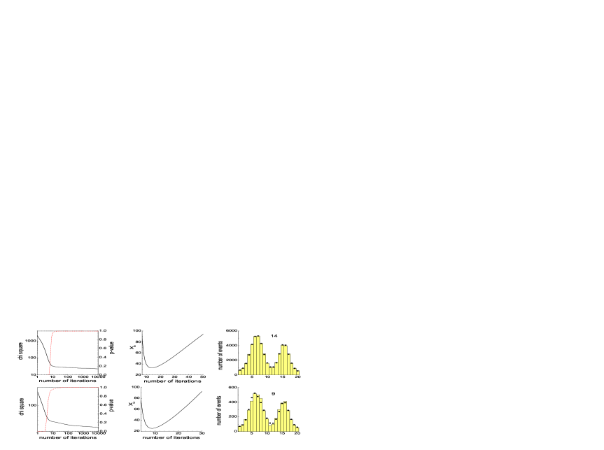
Figure 3: $\chi^{2}$ and $p$-value as a function of the number of iterations (left), $X^{2}$ as a function of the number of iterations (center) and unfolding result after the optimal number of iterations (right). The upper plots correspond to $50,000$ the lower ones to $5,000$ events.

The variation of $\chi^{2}$ as a function of the number of iterations is shown in Fig. 3 top, left hand scale. The corresponding $p$-value (right hand scale) jumps within a few iterations from a negligible value to a value close to one. To judge the quality of the unfolding, we compute the quantity $X^{2}=\Sigma_{i}(\hat{\theta}_{i}-\theta_{i})^{2}/\theta_{i}$ which is available in toy experiments. It is difficult to estimate the range of values of $X^{2}$ that correspond to acceptable solutions, but qualitatively the agreement of the unfolded histogram with the true histogram improves with decreasing $X^{2}$. The dependence of $X^{2}$ from the iteration number is displayed at the top center of the same figure. The minimum is reached at $14$ iterations with a $p$-value of $0.98$ but there is little change between $8$ and $16$ iterations. The corresponding unfolding result is shown on the right hand side. Repeating the same experiment with ten times less events, i.e. $5,000$, we obtain the results displayed at the bottom of Fig. 3. Here the best agreement is reached after $9$ iterations.

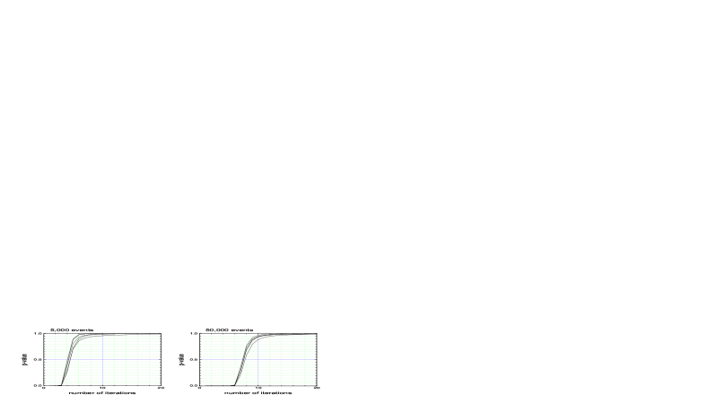
Figure 4: $P$-value as a function of the number of iterations.

The study is repeated for $5$ different samples. The $p$-values are shown as a function of the number of iterations in Fig. 4. All curves start rising nearly at the same iteration, remain close to each other at the beginning but separate at large $p$-values. With $5,000$ events the lowest value of the test quantity $X^{2}$ is always obtained for $8$ or $9$ iterations, while the corresponding $p$-values vary because of the small slopes near $p$-values of one. Therefore, we should base the cut of the chosen number of iterations on a lower $p$-value. The following choice has proven to be quite stable and efficient: We stop the iteration at twice the value at which the $p$-value crosses the $0.5$ line. For the left hand plot with $5,000$ events the crossing is close $4.5$ and thus $9$ iterations should be performed. With $50,000$ events this criterion leads to a choice of $15$ iterations. Actually, from the $X^{2}$ variation, acceptable values are located between $11$ and $16$ iterations. In Table 1 the results for the same distribution but different number of bins of the observed and the unfolded histogram and for different resolutions $\sigma$ are summarized. From left to right the columns contain the number of generated events, the number of bins in the observed and the true histograms, the standard deviation of the Gaussian response function, the number of applied iterations as based on the stopping criterion, $X^{2}$, the corresponding $p$-value, the number of iterations that minimizes $X^{2}$ and the minimal value of $X^{2}$. In each case two independent toy experiments have been performed. The results from the second one are given in parentheses. They are close to those of the first one. In all cases the recipe for the choice of the number of iterations leads in most cases to very sensible results. The $p$-values are close to $1$ in most cases and always above $0.95$.

For the resolution $0.1$ the optimal number of iterations and also the $X^{2}$ values differ considerably from the those found by the stopping criterion. The visual inspection shows however that the unfolded distributions that correspond to the stopping prescription agree qualitatively well with the true distributions. For comparison, the example with $50,000$ events and resolution $0.1$ has also been repeated with a likelihood fit and entropy penalty regularization. The regularization constant was varied until the minimum of $X^{2}$ was obtained. The results was $X^{2}=159$ significantly larger than the value $91$ obtained with iterative unfolding. With the prescription $\Delta\chi^{2}=1$ [15], $X^{2}=873$ was obtained. Regularization with a curvature penalty is not suited for this example. Here the best value of $X^{2}$ is $700$.

Table 1: Test of the $p$-value cut

events	bins	$\sigma$	$\#$	$X^{2}$	$p$-value	$\#_{best}$	$X_{best}^{2}$
50000	40/20	0.07	15 (15)	33 (40)	0.989 (0.986)	15 (14)	33 (40)
5000	40/20	0.07	9 (8)	25 (39)	0.958 (0.980)	9 (9)	25 (39)
50000	40/14	0.07	18 (16)	25(32)	0.978 (0.989)	16 (17)	25 (32)
5000	40/14	0.07	9 (10)	27 (40)	0.997 (0.971)	10 (8)	26 (38)
50000	40/30	0.07	13 (13)	44 (45)	1.000 (1.000)	14 (15)	44 (44)
5000	40/30	0.07	7 (7)	28 (39)	0.997 (1.000)	8 (8)	27 (39)
50000	40/20	0.05	8 (8)	31 (21)	1.000 (1.000)	7 (11)	31 (21)
5000	40/20	0.05	5 (6)	9 (22)	0.997 (0.971)	6 (5)	9 (20)
50000	40/20	0.10	33 (33)	143 (148)	1.000 (1.000)	205 (176)	91 (108)
5000	40/20	0.10	15 (18)	100 (57)	1.000 (0.985)	23 (23)	77 (52)
50000	80/20	0.7	15 (15)	32 (37)	0.991 (0.985)	14 (15)	32 (37)
5000	80/20	0.7	8 (8)	26 (36)	0.970 (0.999)	7 (8)	26 (36)

4.2.1 Interpolation for fast converging iterations

In situations where the response function is narrow, usually the iteration sequence converges quickly to a reasonable unfolded histogram, sometimes after a single iteration. Then one might want to stop the sequence somewhere between two iterations. This is possible with a modified unfolding function. We just have to introduce a parameter $\beta>0$ into (6):

$$\hat{\theta}_{j}^{(k+1)}=\left[\sum_{i=1}^{M}A_{ij}\hat{\theta}_{j}^{(k)}\frac{\hat{d}_{i}}{d_{i}^{(k)}}\left/\alpha_{j}\right.+\beta\hat{\theta}_{j}^{(k)}\right]\;\left/(1+\beta)\right..$$ (7)

The value $\beta=0$ produces the original sequence (6), with $\beta=1$ the convergence is slowed down by about a factor of two and in the limit where $\beta$ approaches infinity, there is no change. It is proposed to choose $\beta$ such that at least $5$ iteration steps are performed.

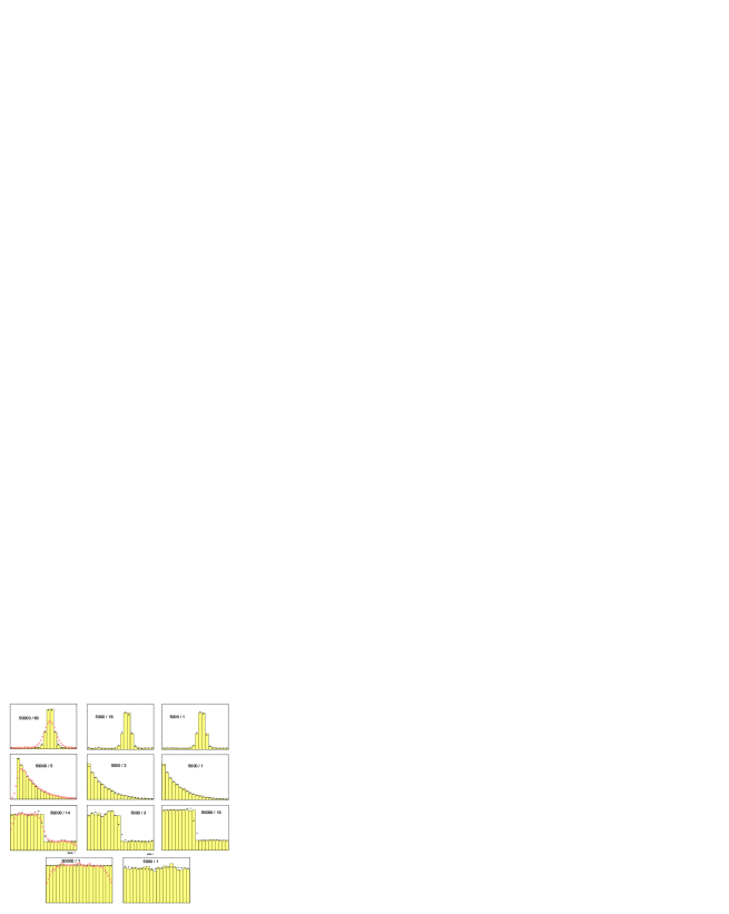
Figure 5: Unfolding results (squares) for different distributions. The shaded histogram corresponds to the input to the detector, the hollow circles to the observed histogram. The number of generated events and the number of applied iterations are indicated.

4.3 Subjective elements

Unfolding is not an entirely objective procedure. The choice of the method and the kind of regularization depend at least partially on personal taste. For a given value of $\chi^{2}$ there exist an infinite number of unfolded histograms. There is no objective criterion which would allow us to choose the best solution. Given the R-L iterative unfolding, with the stopping criterion as defined above and a uniform starting distribution all parameters are fixed, but in some rare situations it may make sense to modify the standard method.

4.3.1 Choice of the starting distribution

Instead of a uniform histogram we may choose a different starting histogram. As long as the corresponding distribution shows little structure, the unfolding result will not be affected very much. If we start in our Example 1 ($50,000$ events) with an exponential distribution $f(x)=e^{-x}$ the unfolded histogram is hardly distinguishable from that with a uniform starting distribution. The difference is less than  $1\%$ in all bins except for the two border bins with only about $60$ entries where it amounts to $2\%$. In both cases $15$ iterations are required.

For an input distribution that is close to the true distribution, the results are in most cases again very similar to those of the uniform input distribution, but of course the number of required iterations is reduced to one ore two. The situation is different for distribution with sharp structures, for instance, if there is a narrow peak with a small smooth background. Starting with a uniform distribution a large number of iterations is required which may lead to oscillations in the background region. This unpleasant effect is avoided if we start with a distribution that includes a peak structure and where only few iterations are necessary.

We have to be careful when choosing a starting distribution different from a monotone function. Only statistically well established structures should be modeled in the starting distribution.

The starting distribution can be obtained by fitting a polynomial, spline functions or another sensible parametrization to the data with the method described in Ref. [19].

4.3.2 Manual smoothing

In the specific example with a narrow peak which we discuss below, starting with a uniform distribution we can also avoid the oscillations if we replace the oscillating part in the true input histogram by a smooth distribution before the last iteration step.

5 Examples with various distributions

We test the R-L unfolding and the stopping criterion with four different distributions, a single peak distribution, an exponential distribution, a step distribution and a uniform distribution. The results are displayed in Fig. 5. The number of events and the number of iterations are indicated in the plots. The starting true function is uniform, except for the last column where a rough guess of the true distribution is used. The input histogram is shaded, the unfolded histogram is indicated by squares and the observed histogram is plotted as circles in the left hand graphs.

Example 2: Single narrow peak

We turn now to a more difficult problem and consider a distribution of $40,000$ events distributed according to $N(x|0.6;0.05)$ and $10,000$ events distributed uniformly. The Gaussian response function with $\sigma=0.07$ is wider than the peak. There is a problem because for the flat region we would be satisfied with few iterations while the peak region requires many iterations. Here $\operatorname{about}$ $60$ iterations are needed because relatively high frequencies are required to model the narrow peak. We get $\chi^{2}=27$ while the value of $\chi_{0}^{2}$ after $100,000$ iterations is $20.6$. The unfolded histogram is shown in Fig. 5 top left together with the smeared histogram and the true histogram. The peak is well reproduced. The corresponding results for $5,000$ events is shown at the center of the first row. The right hand plot is obtained with a modified input distribution for the last iteration. The unfolding result after $18$ iterations is used as input, but the flat region is replaced by a uniform distribution and one additional iteration is applied. In this way the artificial oscillations in the background region are reduced.

To test the effect of an improved starting distribution, a superposition of a quadratic basic spline function (b-spline) and a uniform distribution was fitted to the data. Four parameters were adjusted, two normalization parameters, the location and the width of the b-spline bump. With this starting distribution, after a single iteration the input distribution is almost perfectly reproduced. The test quantity $X^{2}$ is $47$ compared to $216$ with a uniform starting distribution.

Example 3: Exponential distribution

$50,000$ events are generated in the interval $1<x<5$ according to an exponential distribution $f(x)=e^{-x}$ and $\sqrt{x}$ is smeared with a Gaussian resolution of $\sigma=0.1$ which means that the smearing of $x$ increases proportional to $\sqrt{x}$. The events are observed in the interval $0.5<x^{\prime}<5$ and distributed into $40$ bins. The convergence is rather fast because the distribution is smooth even though we start with a uniform true distribution. We stop after $5$ iterations and get $\chi^{2}=31.5$ which corresponds to a $p$-value of $0.996$. The results are shown in the second row of Fig. 5. In fact the agreement of the unfolded distribution improves slightly with additional iterations and is optimum after $7$ iterations. With $5,000$ events the convergence is faster and a reasonable agreement is obtained after $3$ iterations. Starting with a first guess of an exponential distribution the result slightly improves (right hand plot).

Example 4: Step function

A step function is rather exotic. The sharp edge is not easy to reconstruct. We locate the edge at the center of the interval and superpose two uniform distributions containing $40,000$ events in the interval $0<x<0.5$ and $10,000$ events in the interval $0.5<x<1$ with the resolution $\sigma=0.05$. The unfolding results shown in the third row of Fig. 5 are disappointing. The $p$-value of $\ 0.99$ is reached after $25$ iterations with $\chi^{2}=20.63$ ($\chi_{0}^{2}=12.42$). A problem is that to model the sharp edge, many iterations are required while for the flat regions oscillations start after a few iterations. However if we replace the uniform starting distribution by the result displayed in the left hand plot replacing the $16$ bins of the flat region by uniform distributions the result (right hand plot) near the edge is not improved

Example 5: Uniform distribution

A uniform distribution is easy to unfold. $50,000$ events generated in the interval $0<x<1$ with a Gaussian resolution of $\sigma=0.1$ and observed in the same interval are unfolded. As the iteration starts with a uniform distribution, no iteration is necessary and the result is optimal with a $p$-value close to one. The initial value of $\chi^{2}$ is $26.4$ and the minimum value is $19.3$ corresponding to the strongly oscillating ML solution. In the case of $5,000$ events $1$ iteration is applied.

Table 2: Test of the stopping criterion

case	1 peak			2 peak			exponential			step			uniform
	$\chi^{2}$	$X^{2}$	#	$\chi^{2}$	$X^{2}$	#	$\chi^{2}$	$X^{2}$	#	$\chi^{2}$	$X^{2}$	#	$\chi^{2}$	$X^{2}$	#
50,000	27	216	60	31	33	15	29	20	10	24	600	14	26	3	0
50,000 best	29	209	51	31	33	15	30	19	7	18	488	48	26	3	0
5,000	32	167	18	37	25	9	43	7	2	37	104	3	45	6	1
5,000 best	29	71	70	37	25	9	43	7	2	33	96	6	45	6	1

5.0.1 Test of the stopping criterion

In Table 2 we compare the result obtained with the stopping criterion to the result obtained with the optimal number of iterations (denoted by best in the table). In all cases the iteration starts with a uniform distribution. The agreement with the observed distribution, indicated by $\chi^{2}$, the compatibility of the unfolded distribution with the input distribution, measured with $X^{2}$ and the number of applied iterations are given. The stopping criterion produces very satisfactory results in all cases. With the exception of the single peak distribution with $5,000$ events, it is close to the optimum. Here the observed discrepancy between the number of iterations from the stopping criterion and the number derived from the minimum of $X^{2}$ is due to the fact that the distribution consists of a flat region where few iteration are needed and the peak region which requires many iteration to converge to an optimal result. Nevertheless also the solution with $18$ iteration is satisfactory.

6 Summary, conclusions and recommendations

Iterative unfolding with the R-L approach is extremely simple, independent of the number of dimensions, efficiently damps oscillations of correlated histogram bins and needs little computing time. A general stopping criterion has been introduced that fixes the number of iterations, e.g. the regularization strength, that should be applied. It has a simple statistical interpretation. Its stability has been demonstrated for five different distributions, two different event numbers, two different experimental resolutions and three binnings. The results are very satisfactory. The present study should be extended to more distributions with varying statistics and binning and also be applied to higher dimensions.

In most problems a uniform distribution should be used as starting distribution, but the dependence on its shape is negligible as long as this distribution does not contain pronounced structures. In cases where the observed distribution indicates that there are sharp structures in the true distribution, the iterative method permits to implement these in the input distribution. In this way the number of iterations is reduced and oscillations are avoided.

Standard errors, as we associate them commonly in particle physics to measurements, cannot be attributed to explicitly regularized unfolded histograms. We propose to indicate the precision of the graphical representation of the result qualitatively in a way that is independent of the regularization strength. For a quantitative documentation, the unfolding results without explicit regularization should be published together with an error matrix or its inverse. The widths of the bins of the corresponding histogram have to be large enough to suppress excessive fluctuations.

A quantitative comparison of the R-L unfolding with other unfolding methods is difficult, because in most of them a clear prescriptions for the choice of the regularization strength is missing or doubtful. A sensible comparison requires similar binning and regularization strengths in all methods. The latter could be measured with the $p$-value. Independent of the unfolding method that is used, in publications the values of $\chi^{2}$ obtained with and without regularization should be given to indicate the regularization strength and the reliability of the unfolded distribution.

Whenever it is possible to parametrize the true distribution, the parameters should be fitted directly.

Appendix 1: The problem of the error assignment

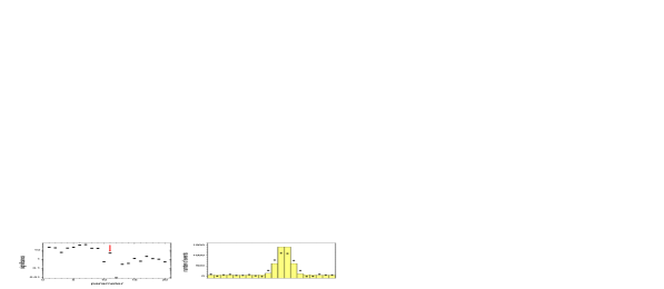
Figure 6: Error assignment in regularized LSFs.

In most unfolding schemes the oscillations are suppressed, either by introduction of a penalty term in the fit, or by reduction of the effective number of parameters [22]. Both approaches constrain the fit and thus reduce the errors. As a consequence the assigned uncertainties do not necessarily cover the true distribution. An example is shown in Fig. 6 right hand side. The parameters of the LS fit have been orthogonalized with a singular value decomposition (SVD) [17]. The left hand plot shows the significance of the parameters which is defined as the ratio of the parameter and its error as assigned by the fit. The $20$ parameters are ordered with decreasing eigenvalues. A smooth cut is applied at parameter $\varepsilon_{c}=11$. Contributions are then weighted by $\phi(\varepsilon)=\varepsilon/(\varepsilon+\varepsilon_{c)}$. In this way oscillations are suppressed that might be caused by an abrupt cut, similar to Gibbs oscillations as observed with Fourier approximations [17, 22]. Obviously the number of $11$ effectively used parameters is insufficient to reproduce the peak and the true distribution is excluded. With the addition of further parameters oscillations start to develop. The problem is especially severe with low event numbers. With $10$ times more events the discrepancy between the true distribution and the unfolded one is considerably reduced.

Regularization with a curvature penalty reduces the statistical errors even in the limit where the resolution is perfect. The errors presented by an experiment that suffers from a limited resolution may be smaller than those of a corresponding experiment with an ideal detector where unfolding is not required.

Appendix 2: The documentation of the results

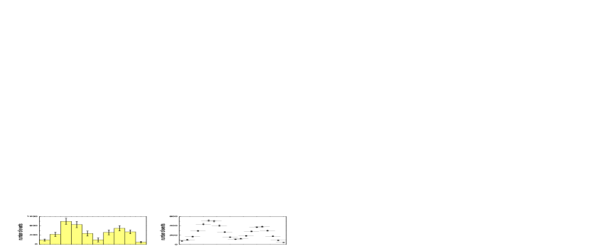
Figure 7: Presentation of an unfolding result.

In the following we present a possible way to document unfolding results such that they can be compared to theoretical predictions and to other experiments.

The left hand plot of Fig. 7 shows the result of a ML fit of the content of the $10$ bins of a histogram without explicit regularization for Example 1 with $5,000$ events. The errors are indicated. They are large due to the strong negative correlation between adjacent bins which amounts to $80\%$. The fitted values together with the error matrix can be used for a quantitative comparison with predictions. Instead of the error matrix its inverse could be presented. The inverse is in fact the item that is required for parameter fitting. Even more information is contained in the combination of the data vector and the response matrix. These items, however, require some explanation to non-experts.

The right hand side of Fig. 7 shows a possibility to indicate the precision of an explicitly regularized unfolded histogram. The plot is based on the same data as in the left hand plot. The vertical error bar corresponds to the uncertainty of the bin content neglecting correlations and the horizontal bars indicate the uncertainty in the location of the events. In the absence of acceptance corrections the vertical error of bin $i$ is simply equal to the square root of the bin content, $\sqrt{\theta_{i}}$. If the average acceptance of the events in the bin is $\alpha_{i}$, the error is $\theta_{i}/\sqrt{\alpha_{i}\theta_{i}}$. The horizontal bar indicates the experimental resolution. Such a graph is intended to show the likely shape of the distribution but is not to be used for a quantitative comparison with other results or predictions. It usually overestimates the uncertainties but for an experienced scientist it indicates quite well the precision of a result.

References

- [1] V. B. Anykeev, A. A. Spiridonov and V. P. Zhigunov, Comparative investigation of unfolding methods, Nucl. Instr. and Meth. A303 (1991) 350.
- [2] Proceedings of the PHYSTAT 2011 Workshop on Statistical Issues Related to Discovery Claims in Search Experiments and Unfolding, CERN, Geneva, Switzerland, ed. H. B. Prosper and L. Lyons (2011).
- [3] G. Cowan, A Survey of Unfolding Methods for Particle Physics, http://www.ippp.dur.ac.uk/old /Workshops/02/statistics/proceedings/cowan.pdf
- [4] W. H. Richardson, Bayesian-Based Iterative Method of Image Restoration, JOSA 62 (1972) 55.
- [5] L. B. Lucy, An iterative technique for the rectification of observed distributions, Astronomical Journal 79 (1974) 745.
- [6] L. A Shepp, Y. Vardi, Maximum Likelihood Reconstruction for Emission Tomography, IEEE transactions on Medical Imaging 1 (1982) 113.
- [7] Y. Vardi, L. A. Shepp and L. Kaufmann, A statistical model for positron emission tomography, J. Am. Stat. Assoc. 80 (1985) 8.
- [8] A. Kondor, Method of converging weights - an iterative procedure for solving Fredholm’s integral equations of the first kind, Nucl. Instr. and Meth. 216 (1983) 177.
- [9] H. N. Mülthei and B. Schorr, On an iterative method for the unfolding of spectra, Nucl. Instr. and Meth. A257 (1987) 371.
- [10] H. N. Mülthei, B. Schorr, On properties of the iterative maximum likelihood reconstruction method, Math. Meth. Appl. Sci. 11 (1989) 331.
- [11] G. D’Agostini, A multidimensional unfolding method based on Bayes’ theorem, Nucl. Instr. and Meth. A 362 (1995) 487.
- [12] L. Lindemann and G. Zech, Unfolding by weighting Monte Carlo events, Nucl. Instr. and Meth. A354 (1995) 516.
- [13] M. C. Abreu et al. A 4-dimensional deconvolution method to correct Na38 experimental data, Nucl. Instr. and Meth.A 405 (1998) 139.
- [14] R. Narayan, R. Nityananda, Maximum entropy image restoration in astronomy, Ann. Rev. Astron. and Astrophys. 24 (1986) 127.
- [15] M. Schmelling, The method of reduced cross-entropy - a general approach to unfold probability distributions, Nucl. Instr. and Meth. A340 (1994) 400.
- [16] P. Magan, F. Courbin and S. Sohy, Deconvolution with correct sampling, Astrophys. J. 494 (1998) 472.
- [17] A. Hoecker and V. Kartvelishvili, SVD approach to data unfolding, Nucl. Instr. and Meth. A 372 (1996), 469.
- [18] N. Milke et al. Solving inverse problems with the unfolding program TRUEE: Examples in astroparticle physics, Nucl. Instr. and Meth. A 697 (2013) 133.
- [19] G. Bohm, G. Zech, Introduction to Statistics and Data Analysis for Physicists, Verlag Deutsches Elektronen-Synchrotron (2010), http://www-library.desy.de/elbook.html. G. Bohm and G. Zech, Comparing statistical data to Monte Carlo simulation with weighted events, Nucl. Instr. and Meth. A691 (2012) 171.
- [20] A. N. Tikhonov,On the solution of improperly posed problems and the method of regularization, Sov. Math. 5 (1963) 1035.
- [21] G. D’Agostini, Improved iterative Bayesian unfolding, arXiv:1010.0632v1 (2010).
- [22] V. Blobel, Unfolding methods in particle physics, Proceedings of the PHYSTAT 2011 Workshop on Statistical Issues Related to Discovery Claims in Search Experiments and Unfolding, CERN, Geneva, Switzerland, ed. H. B. Prosper and L. Lyons (2011).