Abstract

A ladder structure of operators is presented for the associated Legendre polynomials and the spherical harmonics showing that both belong to the same irreducible representation of $so(3,2)$. As both are also bases of square-integrable functions, the universal enveloping algebra of $so(3,2)$ is thus shown to be isomorphic to the space of linear operators acting on the $L^{2}$ functions defined on $(-1,1)\times{\mathbb{Z}}$ and on the sphere $S^{2}$, respectively.

The presence of a ladder structure is suggested to be the general condition to obtain a Lie algebra representation defining in this way the “algebraic special functions” that are proposed to be the connection between Lie algebras and square-integrable functions so that the space of linear operators on the $L^{2}$ functions is isomorphic to the universal enveloping algebra.

Keywords: special functions, Lie algebras, square-integrable functions

1 Introduction

Almost all functions with a name have been sometimes included in the category of special functions. Indeed “special” functions as opposed to the “standard” ones could be defined as the functions that are relevant for applications such that someone has given a name to them [1]. In this approach “special” is simply a synonymous of useful.

Following Talman [2] and Truesdell [3] we are restricting here to special functions that belong to a wide but not so inclusive class. Talman relates special functions to representations of elementary groups, showing that in some cases many of their properties have a group representation origin, while Truesdell introduces the idea of “familiar special functions” as a subclass related to a set of formal properties.

We consider thus a set of formal properties in a similar way of Truesdell but taking into account Talman’s ideas too. Special functions we consider depend from one or more continuous variables and one or more discrete variables, they satisfy ordinary linear differential equations of second order and this equation can be factorized by means of ladder operators. In particular, Hermite, Laguerre and Legendre polynomials verify the above properties allowing to prove that: (i) they are unitary irreducible representations (UIR) of a rank one simple Lie algebra, (ii) they determine an orthogonal complete basis of square-integrable functions defined on the same domain and (iii), because of (i) and (ii), the space of linear operators acting on these ${L}^{2}$ functions is isomorphic to the universal enveloping algebra (UEA) of the corresponding Lie algebra [4].

The goal of this paper is to show that these properties are not restricted to the above mentioned one-dimensional cases since the associated Legendre polynomials (ALP) and the spherical harmonics (SH) satisfy the same conditions and verify the same relations (i)-(iii) with an underlying Lie algebra of rank two. Thus, a subclass of special functions, that we call “algebraic special functions”, can be introduced satisfying the above mentioned conditions and properties.

The paper is organized as follows. Section 2 is devoted to present the main properties of the ALP relevant for our discussion. In section 3 we consider the ALP with fixed $m$ and with $l\geq|m|$, that allows us to build up by using of a set of ladder operators a family of UIR of $so(2,1)$ labelled by the parameter $m$. In section 4 we construct, by means of a different set of ladder operators with fixed $l$ the $so(3)$ UIR of dimension $2l+1$, well known in the case of the spherical harmonics $Y_{l}^{m}(x)$. In section 5, starting from the results of the previous sections, the whole Lie algebra $so(3,2)$ and the UIR supported by the complete set of ALP are constructed. Section 6 is devoted to extend the preceeding results to the SH: like for the ALP the defining equation of the SH is related to the Laplace-Beltrami equation of $so(3,2)$ obtained from the differential realization of its second order Casimir and of all its three-dimensional subalgebras. In section 7 the isomorphism between the space of the operators on the $L^{2}$ functions and the UEA of $so(3,2)$ is discussed. Finally, in section 8, some conclusions and comments are included.

2 Associated Legendre polynomials: a selective view

The starting point of the discussion is the factorization method [5, 6] that relates the second order differential equations defining the special functions to the recurrence formulae with first order derivatives. However, the fundamental limitation of this approach is that the problem has been considered from the point of view of differential equations where the indices (normally only one) are considered as parameters [7]. The dependence of the formulas from the indices in iterated applications must thus be introduced by hand.

As proposed in [4] a consistent vector space framework -where the indices are related to operators- allows to define recurrence formulas in an operator way and is more effective in the description of the underlying mathematical structure.

Hermite, Laguerre and Legendre polynomials have been thus consistently reformulated, showing that they are a basis of a well defined unitary representation of a Lie algebra of rank one. At the same time, these functions are a basis of the $L^{2}$ functions defined on the appropriate open connected subsets of the real line [8]. These $L^{2}$ functions belong thus to the same Lie algebra representation such that the space of linear operators acting on them is isomorphic to the UEA (i.e., to the space that has as a basis the ordered monomials constructed on the generators) [4]. Recurrence formulae are related with the algebra generators, while the defining second order differential equation is obtained as a second order Casimir operator $C_{2}$ of the symmetry algebra.

If these properties can be generalized to all those objects having a ladder structure, a global class of familiar special functions could be considered, where the defining differential equation depends on as many parameters as the rank of the underlying algebra.

In this paper we show that at least two relevant 2-dimensional generalizations are possible: the SH and the ALP (for brevity we consider in detail only the ALP and extend at the end the discussion to the SH). Both are found to be UIR of the real form $so(3,2)$ of the rank two Lie algebra $B_{2}$ with $C_{2}=-5/4$.

The ALP we consider are solutions of the general Legendre equation

$$(1-x^{2})\;y^{\prime\prime}-2x\,y^{\prime}+\left(l(l+1)-\frac{m^{2}}{1-x^{2}}\right)\;y=0,$$ (2.1)

with integers (degree) $l\in{\mathbb{Z}}^{\geq 0}$ and (order) $m\in{\mathbb{Z}},$  with $0\leq|m|\leq l$ and $x\in(-1,1)$. The extension from the interval $(-1,1)$ to a generic interval $(a,b)\subset{\mathbb{R}}$ is trivial and will not be discussed here.

Because the ALP are defined with different conventions by different authors, we adopt here the ones of [9], i.e. with $m\geq 0$:

$$P_{l}^{m}(x)\;\;=\;(-1)^{m}(1-x^{2})^{m/2}\frac{d^{m}}{dx^{m}}P_{l}(x)\;,\quad\quad P_{l}^{-m}=(-1)^{m}\;\frac{(l-m)!}{(l+m)!}P_{l}^{m}(x)\,,$$ (2.2)

where the $P_{l}(x)$ are the Legendre polynomials. Many recurrence relations are supported by the ALP suggesting the presence of a hidden large symmetry[10, 9, 11]. Our starting point is the following set of formulae that include first order derivatives:

$$\begin{array}[]{lll}(x^{2}-1)\;P_{l}^{{}^{\prime}m}(x)&=&\sqrt{1-x^{2}}\;P_{l}^{m+1}(x)+m\,x\;P_{l}^{m}(x),\\[8.5359pt] (x^{2}-1)\;P_{l}^{{}^{\prime}m}(x)&=&-(l+m)(l-m+1)\sqrt{1-x^{2}}\;P_{l}^{m-1}(x)-m\,x\;P_{l}^{m}(x),\\[8.5359pt] (x^{2}-1)\;P_{l}^{{}^{\prime}m}(x)&=&-(l+1)\,x\,P_{l}^{m}(x)+(l-m+1)\;P_{l+1}^{m}(x),\\[8.5359pt] (x^{2}-1)\;P_{l}^{{}^{\prime}m}(x)&=&l\,x\;P_{l}^{m}(x)-(l+m)\;P_{l-1}^{m}(x).\end{array}$$ (2.3)

While eq. (2.1) depends from $m^{2}$  only, eqs. (2.2) exhibit a different normalization of the $\{P_{l}^{m}(x)\}$ for  $m>0$  and  $m<0$ . As all the twentieth century physics has shown, symmetry is fundamental in understanding phenomena. Hence, we eliminate this asymmetric normalization rescaling the $P_{l}^{m}(x)$, in partial agreement with the usual normalization of spherical harmonics, defining:

$$T_{l}^{m}(x):=\sqrt{\frac{(l-m)!}{(l+m)!}}\;P_{l}^{m}(x)$$ (2.4)

that will be the basic objects of this paper. This change is essential to highlight the Lie algebra structure hidden behind (2.3). The elements $T_{l}^{m}(x)$  and  $T_{l}^{-m}(x)$  are equal up to a phase in the configuration space, as

$$T_{l}^{-m}(x)=(-1)^{m}\;T_{l}^{m}(x)\;,$$

but –as discussed in the following– they are eigenvectors of different eigenvalues of the Hermitian operator $M$ and thus different vectors in the vector space $\{T_{l}^{m}(x)\}$. Note that, for $m=0$, $T_{l}^{m}(x)$ –as well as $P_{l}^{m}(x)$– coincide with the Legendre polynomials $P_{l}(x)$ .

In terms of $\{T_{l}^{m}(x)\}$ orthogonality and completeness of ALP for fixed $m$ are [11]

$$\int_{-1}^{1}T_{l}^{m}(x)\;\left(l+1/2\right)\;T_{l^{\prime}}^{m}(x)\;dx=\delta_{l\,l^{\prime}}\qquad(l,l^{\prime}\geq|m|),$$ (2.5)

$$\sum_{l=|m|}^{\infty}T_{l}^{m}(x)\left(l+1/2\right)T_{l}^{m}(y)=\delta(x-y).$$ (2.6)

Let us now display the complete operator structure on the set $\{T_{l}^{m}(x)\}$ we need. In consistency with the quantum theory approach, we have to introduce not only the operators $X$ and $D_{X}$ of the configuration space, such that

$$X\,f(x)=x\,f(x),\qquad D_{x}\,f(x)=f^{\prime}(x),\qquad[X,D_{x}]=-1\,,$$

but also two other operators $L$ and $M$ such that

$$L\;T_{l}^{m}(x)=l\;T_{l}^{m}(x)\,,\qquad M\;T_{l}^{m}(x)=\,m\;T_{l}^{m}(x).$$ (2.7)

These operators $L$ and $M$ allow to take into account the changes in the value of the parameters $m$ and $l$ after subsequent applications of eqs. (2.3) (see Ref. [4]). Thus, the operators

$$J_{\pm} := \mp\sqrt{1-X^{2}}\;D_{x}-\frac{X}{\sqrt{1-X^{2}}}\;M,$$ (2.8)

$$K_{+} := -(1-X^{2})\;D_{x}+X\;(L+1),$$ (2.9)

$$K_{-} := (1-X^{2}\,)\;D_{x}+XL$$ (2.10)

give a formal expression of the eqs. (2.3) rewritten as:

$$J_{+}\;T_{l}^{m}(x)\, = \,\sqrt{(l-m)(l+m+1)}\;T_{l}^{m+1}(x),$$ (2.11)

$$J_{-}\;T_{l}^{m}(x) = \,\sqrt{(l+m)(l-m+1)}\;T_{l}^{m-1}(x),$$ (2.12)

$$K_{+}\;T_{l}^{m}(x) = \,\sqrt{(l-m+1)(l+m+1)}\;T_{l+1}^{m}(x),$$ (2.13)

$$K_{-}\;T_{l}^{m}(x) = \,\sqrt{(l+m)(l-m)}\;T_{l-1}^{m}(x).$$ (2.14)

As shown in next sections, consecutive applications of the operators $J_{\pm}$ and $K_{\pm}$ (that in the course of the procedure modify the values of the parameters $l$ and $m$) allow to recover the equation (2.1). The introduction of the operator $L$ and $M$ in (2.8)–(2.10) is irrelevant in eqs. (2.11)–(2.14) since they are diagonal on the $T_{l}^{m}(x)$ and we have taken care to write them always to the right but, as they do not commute with $J_{\pm}$ and $K_{\pm}$, a more complex algebraic scheme appears:

$$[M,L]=0,\quad[M,J_{\pm}]=\pm J_{\pm},\quad[M,K_{\pm}]=0,\quad[L,J_{\pm}]=0,\quad[L,K_{\pm}]=\pm K_{\pm}.$$

The main result of this paper is that factorization is only the first step of a more formal algebraic approach where eq. (2.1) can be reconstructed not only as product of operators but also as Casimir operator of a Lie algebra. Indeed, starting from the operators $J_{\pm}$ and $K_{\pm}$ and their commutators, we obtain a Lie algebra representation of $so(3,2)$ with $C_{2}=-5/4$. The operators $L$ and $M$, above introduced, belong to the Cartan subalgebra and the ALP (as well as the SH) are a basis of this UIR.

The relevance of this result is related from one side to the role of intertwining between differential equations and Lie algebras played by these algebraic special functions and from the other to the fact that the UEA (i.e., the vector space that has as a basis the ordered monomials of the generators) of $so(3,2)$ is isomorphic to the space of the linear operators acting on the corresponding space of square-integrable functions.

3 so(2,1) and associated Legendre polynomials

In this section we prove that the set of APL  $T_{l}^{m}(x)$ with fixed  $m$  and $l\in{\mathbb{Z}}^{\geq|m|}$ supports a $m$-dependent UIR of the discrete series of $so(2,1)$.

First of all let us consider, starting from eqs. (2.13)–(2.14), the factorization approach. The two operators $K_{\pm}$ act on the $\{T_{l}^{m}(x)\}$ by rising and lowering the label $l$ keaping fix the label $m$. Taking into account that the operator $L$ (2.7) takes different values on $T_{l}^{m}(x)$ and $T_{l\pm 1}^{m}(x)$, recurrence relations allow to recover eq. (2.1) by reiterated application. Indeed remembering eqs. (2.9) and (2.10), the relations

$$K_{+}K_{-}\;\,T_{l}^{m}(x)=(l^{2}-m^{2})\;T_{l}^{m}(x)\;,\qquad K_{-}K_{+}\;\,T_{l}^{m}(x)=((l+1)^{2}-m^{2})\;T_{l}^{m}(x)\;,$$

allow to write

$$\,-(1-X^{2})\;\left((1-X^{2})D_{x}^{2}-2XD_{x}+L(L+1)-\frac{1}{1-X^{2}}\;M^{2}\right)\equiv 0,$$ (3.1)

that, disregarding the irrelevant factor $-(1-X^{2})$, never zero in the domain $(-1,+1)$, is the operator form of eq.(2.1).

Alternatively we can introduce the Lie algebra generated by $K_{\pm}$. The commutator and the anticommutator of $K_{\pm}$ act on the space $\{T_{l}^{m}(x)\}$ as

$$[K_{+},K_{-}]\;T_{l}^{m}(x) = -2\left(l+1/2\right)\;\;T_{l}^{m}(x),$$ (3.2)

$$\{K_{+},K_{-}\}\;T_{l}^{m}(x) = 2\left(l(l+1)-m^{2}+1/2\right)\;T_{l}^{m}(x).$$

Defining, as suggested by eq. (3.2),

$$K_{3}:=L+1/2$$ (3.3)

we see that $K_{3}$ togheter with $K_{\pm}$ close a $so(2,1)$ Lie algebra

$$[K_{3},K_{\pm}]=\pm K_{\pm},\qquad[K_{+},K_{-}]=-2K_{3},$$ (3.4)

with Casimir operator related to $m$:

$${\cal C}_{2}\;T_{l}^{m}(x)\equiv\left(K_{3}^{2}-\frac{1}{2}\{K_{+},K_{-}\}\right)\;\,T_{l}^{m}(x)=(m^{2}-1/4)\;T_{l}^{m}(x)\;.$$ (3.5)

As $m=0,\pm 1,\pm 2\dots$ the double valued discrete UIR of $so(2,1)$ are obtained with ${\cal C}_{2}\equiv m^{2}-1/4=\,-1/4,\,3/4,\,15/4,\dots$ [12]. As $l\geq|m|$ the spectrum of the operator $K_{3}$ is related to the parameter $m$, and has the eigenvalues $1/2+|m|,3/2+|m|,5/2+|m|,\dots$

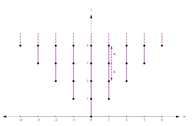
Figure 1: Classification of the ALP  $T_{l}^{m}(x)$ (black points) in terms of the UIR, $U^{m}$, of $so(2,1)$ labeled by $m$ (vertical lines). The operator $K_{3}$ is diagonal with eigenvalue $l+1/2$. The action of the operators $K^{\pm}$ on $T_{3}^{1}(x)$ is also displayed. Note that $U^{m}$ and $U^{-m}$ are equivalent.

Summarizing, the set of ALP  $T_{l}^{m}(x)$ with any fixed $m\in{\mathbb{Z}}$ and $l=|m|,|m|+1,|m|+2,\dots$ supports the double valued UIR, $U^{m}$, of $so(2,1)$ of the discrete series (Figure 1).

Taking now into account the differential representation of the operators (2.9) and (2.10) we see also that the Casimir (3.5) of the $so(2,1)$ algebra reproduces eq. (3.1), i.e., up to the irrelevant global factor $(1-X^{2})$, the operator form of the generalized Legendre equation (2.1):

$${\cal C}_{2}-(M^{2}-1/4)=\,(1-X^{2})\;\left((1-X^{2})D_{x}^{2}-2XD_{x}+L(L+1)-\frac{1}{1-X^{2}}\;M^{2}\right)\equiv 0.$$

4 so(3) and associated Legendre polynomials

Let us now consider the structure related with the operators $J_{\pm}$. They do not change the value of  $l$ but they are, as shown by eqs. (2.11)–(2.12), the well known rising and lowering operators of the rotation algebra $so(3)$ in the representation $l$.

Again the Legendre equation can be easily recovered from the recurrence relations. Indeed, we have from eqs. (2.11) and (2.12)

$$J_{\pm}J_{\mp}\;T_{l}^{m}(x)=(l\pm m)(l\mp m+1)\;T_{l}^{m}(x),$$ (4.1)

that in the differential representation (2.8) is written

$$J_{\pm}J_{\mp}\;T_{l}^{m}(x)=\left(-(1-X^{2})D_{x}^{2}+2XD_{x}+\frac{X^{2}}{1-X^{2}}\;M^{2}\pm M\right)\;T_{l}^{m}(x)\;.$$ (4.2)

Comparing expressions (4.1) and (4.2), the operator form of the generalized Legendre equation (2.1) is easy recovered

$$(1-X^{2})D_{x}^{2}-2XD_{x}+L(L+1)-\frac{1}{1-X^{2}}M^{2}\;=0.$$

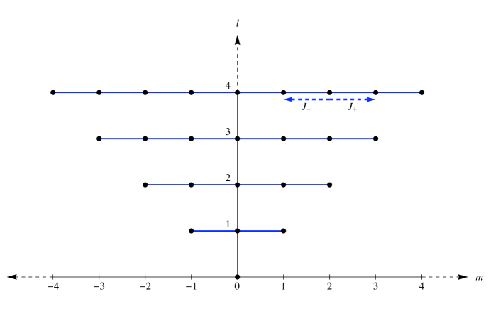
Figure 2: Classification of the ALP $T_{l}^{m}(x)$ (black points) in terms of the IUR, $U^{l}$, of $so(3)$ (horizontal segments). The operator $J_{3}$ is diagonal with eigenvalue $m$. The action of the operators $J_{\pm}$ on $T_{4}^{2}(x)$ is displayed.

As in the preceeding section, let us now introduce the Lie algebraic approach. From eqs. (4.1) commutator and anticommutator are

$$[J_{+},J_{-}]\;T_{l}^{m}(x) = 2\,m\;T_{l}^{m}(x),$$

$$\{J_{+},J_{-}\}\;T_{l}^{m}(x) = 2\left(l(l+1)-m^{2}\right)\;T_{l}^{m}(x),$$

and, defining

$$J_{3}:=M,$$ (4.3)

we get the $so(3)$ algebra

$$[J_{3},J_{\pm}]=\pm J_{\pm}\,,\quad\qquad[J_{+},J_{-}]=2J_{3}\;$$ (4.4)

with Casimir

$${\cal C}_{2}\;T_{l}^{m}(x)=\left(J_{3}^{2}+\frac{1}{2}\{J_{+},J_{-}\}\right)\;T_{l}^{m}(x)=\,l(l+1)\;T_{l}^{m}(x)\,.$$

Starting now from the differential representation of the operators $J_{\pm}$ (2.8), we can rewrite

$${\cal C}_{2}-L(L+1)=-\left((1-X^{2})D_{x}^{2}-2XD_{x}+L(L+1)-\frac{1}{1-X^{2}}\;M^{2}\right)\equiv 0,$$

i.e., the operator equation (2.1) now obtained from the Casimir of the subalgebra $so(3)$ with fixed $l$.

Summarizing, the set of ALP $T_{l}^{m}(x)$ with any fixed $l\in{\mathbb{Z}}$ and $m=-l,-l+1,\dots,l-1,l$  supports the unitary irreducible representation $U^{l}$ of $so(3)$, as shown in the Figure 2.

5 so(3,2) and associated Legendre polynomials

Starting from the operators (2.8)–(2.10) and their actions (2.11)–(2.14) on the vector space of the APL $T_{l}^{m}(x)$, we generalize to the full vector space $\{T_{l}^{m}(x)\}$ the algebraic structures discussed in sections 3 and 4.

Indeed, as both for $m$ or $l$ fixed we have found an underlying algebra, we can look for a global Lie algebra of which both $so(2,1)$ and $so(3)$ are subalgebras, such that the set of all the ALP $\{T_{l}^{m}(x)\}$ supports a representation of this algebra. As the operators $K_{+}$ and $J_{\pm}$ applied to $T_{0}^{0}(x)=1$ generate the full space $\{T_{l}^{m}(x)\}$

$$T_{l}^{\pm m}(x)=\frac{1}{l!}\;\sqrt{\frac{(l-m)!}{(l+m)!}}\;(J_{\pm})^{m}\;(K_{+})^{l}\;T_{0}^{0}(x),\qquad m\geq 0\,,$$

hence the representation, if it exists, is irreducible.

Since $\langle K_{3},K_{\pm}\rangle$ and $\langle J_{3},J_{\pm}\rangle$ should be subalgebras, we have to consider only the mixed commutators. So, defining

$$R_{\pm}:=[K_{\pm},J_{\pm}]$$

we obtain from (2.11)–(2.14)

$$R_{+}\;T_{l}^{m}(x)=\sqrt{(l+m+2)(l+m+1)}\;T_{l+1}^{m+1}(x),$$ (5.1)

$$R_{-}\;T_{l}^{m}(x)=\sqrt{(l+m)(l+m-1)}\;T_{l-1}^{m-1}(x),$$ (5.2)

and from eqs. (2.8)–(2.10) the differential form of the operators $R_{\pm}$

$$R_{+}=-X\;\sqrt{1-X^{2}}\;D_{x}-\frac{1}{\sqrt{1-X^{2}}}\;M-\sqrt{1-X^{2}}\;(L+1),$$ (5.3)

$$R_{-}=X\;\sqrt{1-X^{2}}\;D_{x}-\frac{1}{\sqrt{1-X^{2}}}\;M-\sqrt{1-X^{2}}\;L.$$ (5.4)

In a similar way to the previous cases the general Legendre equation (2.1) can be obtained by means of the factorization method applying the recurrence relations $R_{\pm}R_{\mp}$ to $T_{l}^{m}(x)$.

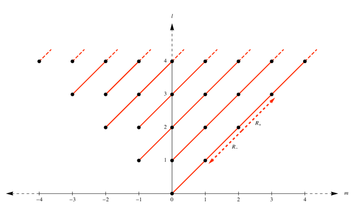
Figure 3: Classification of the ALP $T_{l}^{m}(x)$ (black points) in terms of the UIR of $so(2,1)\equiv\langle R_{\pm},R_{3}\rangle$ (inclined lines). The operator $R_{3}$ is diagonal with eigenvalues $l+m+1/2$. The action of the operators $R^{\pm}$ on $T_{2}^{2}(x)$ is also displayed.

Moreover, as

$$[R_{+},R_{-}]=-4(L+M+1/2),\qquad$$ (5.5)

we can define $R_{3}:=L+M+1/2$ and find that $R_{\pm}$ and $R_{3}$ span a $so(2,1)$ algebra

$$[R_{+},R_{-}]=-4R_{3},\qquad[R_{3},R_{\pm}]=\pm 2R_{\pm}\,.$$ (5.6)

The Casimir gives

$$R_{3}^{2}-\frac{1}{2}\{R_{+},R_{-}\}+\frac{3}{4}\equiv 0$$

that, written in terms of the differential form (5.3) and (5.4) of $R_{\pm}$ reproduces again, up to an irrelevant $X^{2}$ global factor, the operator Legendre equation (2.1)

$$R_{3}^{2}-\frac{1}{2}\{R_{+},R_{-}\}+\frac{3}{4}\,\equiv\,X^{2}\left((1-X^{2})D_{x}^{2}-2XD_{x}+L(L+1)-\frac{1}{1-X^{2}}\;M^{2}\right)=0,$$

that can be thus derived also from the subalgebra $\langle R_{\pm},R_{3}\rangle$, i.e., $so(2,1)$ with $l-m$ fixed. Moreover, rescaling the generators as

$$R_{i}\to R^{\prime}_{i}=\frac{1}{2}R_{i}\,,$$

eqs. (5.6) reproduce the standard form for the Lie commutators of $so(2,1)$ as reported in eq. (3.4) and thus for all these (infinite) representations of $so(2,1)$ the Casimir ${\cal C}_{2}$ is $-3/16$. Since ${\cal C}_{2}=k(k-1)$ the maximal weight is $k=1/4$ or $3/4$. The spectrum of $R_{3}$ is indeed  $1/2,5/2,9/2,\dots$  when  $l+m$  is even and  $3/2,7/2,11/2,\dots$ when $l+m$ is odd (see Figure 3).

In a similar way we define two other new operators, denoted by $S_{+}$ and $S_{-},$

$$S_{\pm}:=[K_{\pm},J_{\mp}].$$

Their actions on the ALP $T_{l}^{m}(x)$ are

$$S_{+}\;T_{l}^{m}(x)=\sqrt{(l-m+2)(l-m+1)}\;T_{l+1}^{m-1}(x),$$ (5.7)

$$S_{-}\;T_{l}^{m}(x)=\sqrt{(l-m)(l-m-1)}\;T_{l-1}^{m+1}(x)$$ (5.8)

and their differential forms

$$S_{+}=X\sqrt{1-X^{2}}\;D_{x}-\frac{1}{\sqrt{1-X^{2}}}\;M+\sqrt{1-X^{2}}\;(L+1),$$

$$S_{-}=-X\sqrt{1-X^{2}}\;D_{x}-\frac{1}{\sqrt{1-X^{2}}}\;M+\sqrt{1-X^{2}}\;L.$$

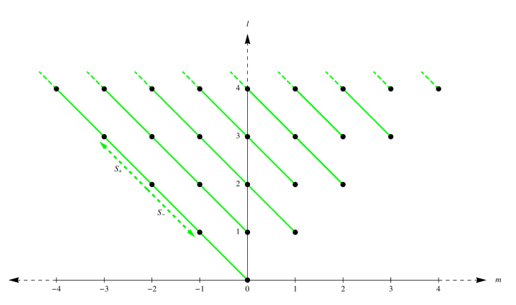
Figure 4: Classification of the ALP $T_{l}^{m}(x)$ (black points) in terms of the UIR of $so(2,1)\equiv\langle S_{\pm},S_{3}\rangle$ (inclined lines). The operator $S_{3}$ is diagonal with eigenvalues $l-m+1/2$. The action of $S^{\pm}$ on $T_{2}^{-2}(x)$ is also displayed.

Again, like before, the Legendre equation can be obtained applying the recurrence relations $S_{\pm}S_{\mp}$ to $T_{l}^{m}(x)$. The situation is similar to the previous case also for the algebraic approach: in analogy with (5.6), defining $S_{3}:=L-M+1/2$, we have

$$[S_{+},S_{-}]=-4S_{3},\qquad[S_{3},S_{\pm}]=\pm 2S_{\pm}.$$ (5.9)

By inspection, $\langle S_{\pm},S_{3}\rangle$ is a new $so(2,1)$ algebra obtained from $\langle R_{\pm},R_{3}\rangle$ with the substitution $M\to-M$. It has thus the same representation with Casimir ${\cal C}_{2}=-3/16$ than $\langle R_{\pm},R_{3}\rangle$ (see Figures 3 and 4) and allows to obtain again the Legendre equation (2.1).

So, we have four set of operators $\{J_{\pm},J_{3}\}$, $\{K_{\pm},K_{3}\}$, {$R_{\pm},R_{3}\}$, and $\{S_{\pm},S_{3}\}$ generating the first one a $so(3)$ algebra and each of the other three a $so(2,1)$ algebra. All together these operators close a bigger Lie algebra containing all these four algebras as subalgebras. First of all notice that

$$R_{3}=J_{3}+K_{3},\qquad S_{3}=-J_{3}+K_{3},$$

hence, the rank of this algebra is two as only two elements of the Cartan subalgebra are independent. From eqs. (2.11)–(2.14), (3.3), (4.3), (5.1), (5.2), (5.7) and (5.8) the crossed commutators between all these generators are easily computed:

$$\begin{array}[]{llll}&[J_{\pm},K_{\pm}]=\pm R_{\pm},&[J_{\mp},K_{\pm}]=\pm S_{\pm},&[J_{3},K_{\pm}]=0,\qquad[J_{3},K_{3}]=0,\\[8.5359pt] &[J_{\pm},R_{\pm}]=0,&[J_{\mp},R_{\pm}]=\pm 2K_{\pm},&[J_{3},R_{\pm}]=\pm R_{\pm},\\[8.5359pt] &[J_{\pm},S_{\pm}]=\pm 2K_{\pm},&[J_{\mp},S_{\pm}]=0,&[J_{3},S_{\pm}]=\mp S_{\pm},\\[8.5359pt] &[K_{\pm},R_{\pm}]=0,&[K_{\mp},R_{\pm}]=\pm 2J_{\pm},&[K_{3},R_{\pm}]=\pm R_{\pm},\\[8.5359pt] &[K_{\pm},S_{\pm}]=0,&[K_{\mp},S_{\pm}]=\pm 2J_{\mp},&[K_{3},S_{\pm}]=\pm S_{\pm},\\[8.5359pt] &[R_{\pm},S_{\pm}]=0,&[R_{\mp},S_{\pm}]=0.&\end{array}$$ (5.10)

From all the commutators (3.4), (4.4), (5.5), (5.9) and (LABEL:so32comm) we are dealing with the noncompact real form $so(3,2)$ of $B_{2}$ which root diagram is displayed in Fig. 5.

The quadratic Casimir operator ${\cal C}^{so(3,2)}_{2}$ can now be evaluated to be $-5/4$ and by means of the differential form of the generators the equation (2.1) is again obtained

$${\cal C}^{so(3,2)}_{2}+5/4\equiv\,X^{2}\left((1-X^{2})D_{x}^{2}-2XD_{x}+L(L+1)-\frac{1}{1-X^{2}}\;M^{2}\right)=0.$$

The general Legendre equation is thus strictly related to $so(3,2)$ since it can be obtained from the quadratic invariant of $so(3,2)$ or, alternatively, from the Casimir of any of its three-dimensional subalgebras.

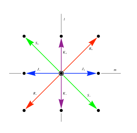
Figure 5: Root system of $B_{2}$. The two-dimensional Cartan subalgebra is represented at the origin.

6 $so(3,2)$ and spherical harmonics

We extend now the discussion to spherical harmonics $Y_{l}^{m}$ that are well known to be related, for $l$ fixed, with a representation of $so(3)$. In this paper we show that the SH $\{Y_{l}^{m}\}$, for all values of $l$ and $m$, support, as the set $\{T_{l}^{m}\}$, the UIR with ${\cal C}_{2}=-5/4$ of $so(3,2)$.

Remember that spherical harmonics ${Y_{l}^{m}(\theta,\phi)}$ are

$$Y_{l}^{m}(\theta,\phi)\;=\;Ne^{{\bf i}m\phi}\;P_{l}^{m}(x),$$

where different normalizations $N$ are considered in different fields of research. To save the correspondence with the ALP (and, in this way, the customary Lie algebra matrix elements) we fix

$$N=\frac{1}{\sqrt{2\pi}}\sqrt{\frac{(l-m)!}{l+m)!}}.$$ (6.1)

Hence, the $Y_{l}^{m}(\theta,\phi)$ are:

$$Y_{l}^{m}(\theta,\phi)\;=\;\frac{1}{\sqrt{2\pi}}\sqrt{\frac{(l-m)!}{(l+m)!}}\;e^{{\bf i}m\phi}\;P_{l}^{m}(x)=\frac{1}{\sqrt{2\pi}}\;e^{{\bf i}m\phi}\;T_{l}^{m}(x),$$

where $x=\cos\theta$ and $\phi$ is the conjugated variable of $m$. Taking into account the normalization constant (6.1), orthogonality and completeness of the $\{Y_{l}^{m}\}$ are [13]

$$\int d\Omega\;\,Y_{l}^{m\;*}\;(\theta,\phi)\;\left(l+1/2\right)\;Y_{l^{\prime}}^{m^{\prime}}(\theta,\phi)\;\;=\;\;\delta_{l\,l^{\prime}}\;\delta_{m\,m^{\prime}}\;,$$

$$\sum_{l\,m}\;Y_{m}^{m\;*}\;(\theta,\phi)\;\left(l+1/2\right)\;Y_{l}^{m}(\theta^{\prime},\phi^{\prime})\;=\;\delta\left(\cos\theta-\cos\theta^{\prime}\right)\;\delta(\phi-\phi^{\prime}).$$

With the substitutions $J_{\pm}\to{J_{\pm}}^{\prime}=e^{\pm{\bf i}\phi}J_{\pm}$,   $R_{\pm}\to{R_{\pm}}^{\prime}=e^{\pm{\bf i}\phi}\,R_{\pm}$,  $S_{\pm}\to{S_{\pm}}^{\prime}=e^{\mp{\bf i}\phi}\,S_{\pm}$ and with $K_{\pm}$ remaining invariant all the preceding results obtained for the $\{T_{l}^{m}\}$ can now be easily translated to the $\{Y_{l}^{m}\}$.

7 Operators on $L^{2}$ spaces and UEA

We have shown in the preceding sections that both the ALP and SH are a basis of a representation of $so(3,2)$. In this section we consider as both, the ALP and the the SH, are a basis of the $L^{2}$ functions defined on $(-1,1)\times{\mathbb{Z}}$ and $S^{2}$, respectively. Thus the vector space of the linear operators acting on these $L^{2}$ functions is isomorphic to the UEA of $so(3,2)$. In this way the results presented in [4] for the one-variable square-integrable functions are extended to these two-variable cases.

Again the discussion will be made for the ALP since the extension to the SH is trivial. Let us start from the separable Hilbert space of the square-integrable functions defined on both $E:=(-1,1)\subset{{\mathbb{R}}}$ and ${\mathbb{Z}}$, i.e. ${L}^{2}(E,{\mathbb{Z}})$, direct sum of the Hilbert spaces with $m$ fixed: ${L}^{2}(E,{\mathbb{Z}})=\bigcup_{m=-\infty}^{\infty}\;{L}^{2}(E,m)$.

A basis for ${L}^{2}(E,{\mathbb{Z}})$ is $\{|x,m\rangle\}$ ($-1<x<1,m\in{\mathbb{Z}}$). Orthonormality and completeness relations are

$$\langle x,m|x^{\prime},m^{\prime}\rangle\;=\;\delta(x-x^{\prime})\,\delta_{m\,m^{\prime}},\qquad\sum_{m}\,\int_{-1}^{+1}dx\,|x,m\rangle\,\langle x,m|\;=\;{\cal I}.$$ (7.1)

As the $\{T_{l}^{m}(x)\}$ satisfy eqs. (2.5) and (2.6) we can now define inside the Hilbert space a new basis $\{|l,m\rangle\}$ with $l\geq|m|$

$$|l,m\rangle:=\int_{-1}^{+1}|x,m\rangle\,\sqrt{l+1/2}\;\,T_{l}^{m}(x)\,dx\;.$$ (7.2)

such that

$$\langle l,m|l^{\prime},m^{\prime}\rangle\;=\;\delta_{l\,l^{\prime}}\,\delta_{m\,m^{\prime}}\,,\qquad\sum_{l,m}|l,m\rangle\;\langle l,m|\;=\;{\cal I}.$$

Thus the $T_{l}^{m}(x)$ play the role of transition matrices and, as the space is real, can be written as

$$T_{l}^{m}(x)=\frac{1}{\sqrt{l+1/2}}\;\langle x,m|l,m\rangle=\frac{1}{\sqrt{l+1/2}}\;\langle l,m|x,m\rangle\;.$$ (7.3)

In this way, in analogy with [4], an arbitrary vector $|f\rangle\,\in L^{2}(E,{\mathbb{Z}})$ can be expressed as

$$|f\rangle\;=\;\sum_{m=-\infty}^{\infty}\int_{-1}^{+1}dx\;|x,m\rangle\,\langle x,m|f\rangle\;=\sum_{m=-\infty}^{+\infty}\;\sum_{l=|m|}^{\infty}|l,m\rangle\;\langle l,m|f\rangle$$

and we can describe $|f\rangle$ in two alternative bases by means of the functions $f^{m}(x)$ or the succession $f_{l}^{m}$ :

$$f^{m}(x):=\langle x,m|f\rangle=\sum_{l=|m|}^{\infty}T_{l}^{m}(x)\,f_{l}^{m},\qquad f_{l}^{m}:=\langle l,m|f\rangle=\int_{-1}^{+1}dx\;T_{l}^{m}(x)\,f^{m}(x)\;.$$

In particular, the completeness of the two bases determines the inner product

$$\langle f|g\rangle\;=\sum_{m=-\infty}^{\infty}\;\sum_{l=|m|}^{\infty}\;g_{l}^{m}f_{l}^{m}=\sum_{m=-\infty}^{\infty}\;\int_{-1}^{1}dx\,g^{m}(x)\,f^{m}(x),$$

as well as the Parseval identity

$$\sum_{m=-\infty}^{\infty}\;\sum_{l=|m|}^{\infty}\;[f_{l}^{m}]^{2}=\sum_{m=-\infty}^{\infty}\;\int_{-1}^{1}dx\;[f^{m}(x)]^{2}\;.$$

All the $L^{2}$ functions defined on $(E,{\mathbb{Z}})$ can be written as

$$\sum_{m=-\infty}^{\infty}\;\sum_{l=|m|}^{\infty}\;T_{l}^{m}(x)\;f_{l}^{m},$$

hence they belong to the described UIR of $so(3,2)$. The space of all linear operators that act on $L^{2}(E,{\mathbb{Z}})$ is thus isomorphic the UEA of $so(3,2)$.

The SH case is similar: it can now be discussed substituting (7.1) by the expression

$$\langle\theta,\phi|\theta^{\prime},\phi^{\prime}\rangle\;=\;\delta(\cos\theta-\cos\theta^{\prime})\,\delta{(\phi-\phi^{\prime})},\qquad\int d\Omega\;|\theta,\phi\rangle\,\langle\theta,\phi|\;=\;{\cal I}.$$

and (7.3) by (see Ref. [13])

$$Y_{l}^{m}(\theta,\phi)=\frac{1}{\sqrt{l+1/2}}\;\langle\theta,\phi|lm\rangle=\frac{1}{\sqrt{l+1/2}}\;{\langle lm|\theta,\phi\rangle}^{*}\,.$$

The SH $\{Y_{l}^{m}(\theta,\phi)\}$ as well as all $L^{2}$ functions defined on the sphere $S^{2}$ also support the representation with ${\cal C}=-5/4$ of $so(3,2)$ and the space of linear operators acting on the $L^{2}$ functions defined on the sphere is thus isomorphic to the UEA of $so(3,2)$.

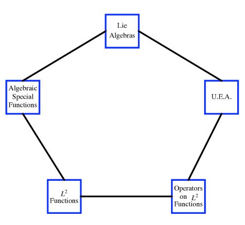
Figure 6: Diagrammatic resume of the philosophy of the paper.

8 Conclusions

Following the ideas of Talman and Truesdell we have introduced a subclass of special functions, we call algebraic special functions, that support a ladder structure. This excludes elementary functions but it includes many of the other special functions which are familiar in physical applications. Their fundamental role seems to be the connection between differential equations, Lie algebras and spaces of $L^{2}$ functions.

Indeed they support a UIR of a Lie algebra and, at the same time, they are a basis in a $L^{2}$ functions space. This shows that the space of the linear operators acting on this $L^{2}$ space is isomorphic to the UEA of the algebra.

In particular, in this paper we discuss ALP and SH. Both are bases of the $L^{2}$ functions defined in the first case in the set $(-1,1)\times{\mathbb{Z}}$ and in the second one in the sphere $S^{2}$. They support a particular representation of $so(3,2)$ hence the operators acting on the $L^{2}$ functions defined in $(-1,1)\times{\mathbb{Z}}$ and in $S^{2}$ belong to the UEA of the $so(3,2)$.

An interesting point is that, in all the cases we have taken into account the commutators (of the algebra) and product (i.e. the factorization method) carry to the same result. It seems that it is necessary to fix both, the Lie algebra and the representation (i.e. the product) to determine the properties of differential equations we started from. This should imply that for algebraic special functions Casimirs of order higher of two are irrelevant in the sense that they only allow to obtain again the basic differential equation.

The ladder approach is suitable also for no simple Lie algebras. Consider, for instance, Bessel functions. The limit of the ALP to the Bessel functions [14] is associated to the following multiple contractions: 1) contraction of the algebraic ladder structure, i.e., $so(3)$ to the Euclidean algebra of the plane [13], 2) the contraction-limit of the $L^{2}$ functions from the sphere $S^{2}$ to the cylinder, and 3) the corresponding contraction between the operators acting on them.

To test the scheme in a more general case we are working now to connect Jacobi polynomials with a Lie algebra of rank three.

A pictorial description of the ideas behind the approach is displayed in Fig. 6.

References

[1] M Berry, Phys. Today54, 11 (2001).
[2]
J D Talman, Special functions: a group theoretic approach (New York: Benjamin, 1968).
[3]
C Truesdell, Annals in Math. Studies18 (Princeton: Princeton Univ. Press 1948).
[4]
E Celeghini and M A del Olmo, submitted to Annals of Physics 2012;
arXiv: 1205.6353 [math-ph].
[5]
E. Schrödinger, Proc. Roy. Irish Acad. A46, 183 (1940); A47, 53 (1941).
[6] L Infeld and T E Hull, Rev. Mod. Phys.
23, 21 (1951).
[7]
W. Miller, Lie Theory and Special Functions (New York: Academic Pres 1968).
[8] S. Cambianis, Proc. of the Am. Math. Soc.29, 284 (1971).
[9]
F.W.J. Olver, D.W. Lozier, R.F. Boisvert and C.W. Clark, NIST Handbook of Mathematical Functions,
(New York: Cambridge Univ. Press, 2010).
[10]
M. Abramowitz and I. A. Stegun, Handbook of Mathematical Functions (New York: Dover, 1972).
[11]
G. ’tHooft and S. Noobbenhuis, Special Functions and Polynomials
www.phys.uu.nl/~hooft101/GtH_lectures.html.
[12] V.Bargmann, Ann. of Math.48, 368 (1947).
[13]
Wu-Ki Tung, Group Theory in Physics (Singapore: World Scientific 1985).
[14] A. Erd lyi, W. Magnus, F. Oberhettinger and F.G. Tricomi,
Higher Transcendental Functions,
Bateman-Project (New York: McGraw-Hill, 1955).