Maximum Likelihood Algorithms for Joint Estimation of Synchronization Impairments and Channel in MIMO-OFDM System

Abstract

Maximum Likelihood (ML) algorithms, for the joint estimation of synchronization impairments and channel in Multiple Input Multiple Output-Orthogonal Frequency Division Multiplexing (MIMO-OFDM) system, are investigated in this work. A system model that takes into account the effects of carrier frequency offset, sampling frequency offset, symbol timing error, and channel impulse response is formulated. Cramér-Rao Lower Bounds for the estimation of continuous parameters are derived, which show the coupling effect among different impairments and the significance of the joint estimation. We propose an ML algorithm for the estimation of synchronization impairments and channel together, using grid search method. To reduce the complexity of the joint grid search in ML algorithm, a Modified ML (MML) algorithm with multiple one-dimensional searches is also proposed. Further, a Stage-wise ML (SML) algorithm using existing algorithms, which estimate fewer number of parameters, is also proposed. Performance of the estimation algorithms is studied through numerical simulations and it is found that the proposed ML and MML algorithms exhibit better performance than SML algorithm.

I Introduction

The integration of Multiple Input Multiple Output (MIMO) and Orthogonal Frequency Division Multiplexing (OFDM) techniques has become a preferred solution for the high rate wireless technologies due to its high spectral efficiency, robustness to frequency selective fading, increased diversity gain, and enhanced system capacity. The main drawback of OFDM based systems is their susceptibility to synchronization impairments such as Carrier Frequency Offset (CFO), Sampling Frequency Offset (SFO) and Symbol Timing Error (STE) [1], [2].

So far, most studies on OFDM systems have considered synchronization impairments and channel separately [2, 3, 4, 5, 6, 7, 8]. Maximum Likelihood (ML) estimation algorithms for joint estimation of CFO, channel, and STE of an Orthogonal Frequency Division Multiplexing Access (OFDMA) system and Single Input Single Output (SISO)-OFDM system are proposed in [3] and [5], respectively, but SFO is assumed to be zero. Similarly, a joint ML time frequency synchronization and channel estimation algorithm for MIMO-OFDM systems has been proposed in [6] and [7], without considering the effect of SFO. In [4], a pilot-aided joint Channel Impulse Response (CIR), CFO, and SFO estimation scheme has been proposed for MIMO-OFDM systems, assuming a perfect start of frame detection. An ML estimator of SFO and CFO for an OFDM system is developed in [9], but STE is assumed to be zero with perfect channel knowledge. Joint ML estimators for SFO and channel for OFDM systems are proposed in [8], without considering the effect of CFO and STE.

In this paper, we propose ML algorithms for the joint estimation of SFO, CFO, STE, and channel in MIMO-OFDM system. An ML algorithm is proposed, where the multi-dimensional optimization problem for estimating the parameters is reduced to a two-dimensional and a one-dimensional grid search. To reduce the complexity further, a Modified ML (MML) algorithm, which involves only multiple one-dimensional searches, is also proposed. Further, a Stage-wise ML (SML) algorithm using existing algorithms, which estimate fewer number of parameters, is also proposed. Cramér-Rao Lower Bounds (CRLB) for the estimation of continuous parameters are derived, which show the coupling effect among different impairments and the significance of the joint estimation algorithms. Some results of this paper are also presented in [10].

II SYSTEM MODEL

Consider a MIMO-OFDM system with $N_{T}$ transmit antennas and $N_{R}$ receive antennas using Quaternary Phase Shift Keying (QPSK) Modulation and $N$ subcarriers per antenna. The input bit stream is first multiplexed in space and time before being grouped by the serial-to-parallel converter. After Inverse Fast Fourier Transform (IFFT) operation, cyclic prefix (CP) insertion and digital-to-analog conversion, the transmitted signal from ${u^{\mathrm{th}}}$ radio frequency (RF) transmit antenna undergoes fading by the channel before reaching the ${v}^{\mathrm{th}}$ RF receive antenna. Let $T$ be the sampling time of the sampling frequency oscillator at the transmitter. Then the subcarrier spacing is given by $1/(NT)$. The CIR between ${u^{\mathrm{th}}}$ transmit and ${v^{\mathrm{th}}}$ receive antenna is $h_{u,v}(\tau)=\sum_{l=0}^{L_{u,v}-1}{h_{u,v,l}\delta(\tau-\tau_{l})}$, where $h_{u,v,l}$ denotes the channel coefficient, $\tau_{l}$ denotes the $l^{\mathrm{th}}$ channel path delay ($\tau_{l}=lT$), and $L_{u,v}$ denotes the length of CIR, for $u=1,2,3,\ldots,N_{T}$ and $v=1,2,3,\ldots,N_{R}$.

At each receive antenna, a superposition of faded signals from all transmit antennas together with noise is received. Frequency differences between RF oscillators used in the MIMO-OFDM transmitter and receiver, and channel induced Doppler shifts cause a net CFO of $\Delta f_{c}$ in the received signal, where $f_{c}$ is the operating radio carrier frequency of the RF oscillator. Furthermore, at the receiver, the received signal is sampled at $T^{{}^{\prime}}$ where $T^{{}^{\prime}}\neq T$ and $\Delta T=T^{{}^{\prime}}-T$, which results in SFO. The normalized CFO is $\epsilon=\Delta f_{c}NT$ and the normalized SFO is $\eta=\Delta T/T$. The frame arrival detection in OFDM based systems is done using different correlation methods [11, 12, 13]. The main drawback of these methods is that the correlation functions do not produce a sharp peak at the arrival of the frame, which results in difficulty to find the fine frame time arrival instant, causing STE [6]. Let the STE, after start of frame detection, be given by integer number of samples $\theta T$, where $\theta$ is the normalized STE. The fractional part of the timing error is incorporated into the CIR  [14, 15]. We assume all receive antennas experience common synchronization impairments in a single user MIMO-OFDM system [6, 7].

We consider the estimation of impairments during the training block. As the training blocks are usually preceded by long CP in practical applications, we assume that the length of CP is greater than $(L_{m}+\theta_{max}$), where $L_{m}=\max\limits_{u,v}\{L_{u,v}\}$ and $\theta_{max}$ is the maximum STE [3]. The received signal at the ${v}^{\mathrm{th}}$ RF receive antenna is given by

$$r_{v}(n)=\exp(j2\pi\Delta f_{c}nT^{{}^{\prime}})\sum_{u=1}^{N_{T}}\sum_{l=0}^{L_{m}-1}h_{u,v,l}s_{u}(nT^{{}^{\prime}}-\theta T-\tau_{l})+w_{v}(n).$$

where $s_{u}(n)$ is the signal transmitted by the $u^{\mathrm{th}}$ transmit antenna and $w_{v}(n)$ is the complex additive Gaussian noise at the $v^{\mathrm{th}}$ receive antenna with mean zero and variance $\sigma_{w}^{2}$. We have,

$$s_{u}(nT^{{}^{\prime}}-\theta T-\tau_{l})=s_{u}(n(T+\Delta T)-\theta T-\tau_{l})=s_{u}((n_{\eta}-\theta-l)T)$$

$$\exp(j2\pi\Delta f_{c}nT^{{}^{\prime}})=\exp(j2\pi\varepsilon n(T+\Delta T)/NT)=\exp(j2\pi\varepsilon_{\eta}n/N).$$

where $\varepsilon_{\eta}=\varepsilon(1+\eta)$, and $n_{\eta}=n(1+\eta).$ Thus,

$$r_{v}(n)=\exp(j2\pi\varepsilon_{\eta}n/N)\sum_{u=1}^{N_{T}}\sum_{l=0}^{L_{m}-1}h_{u,v,l}s_{u}(n_{\eta}-\theta-l)+w_{v}(n).$$ (1)

From (1), it can be observed that there is coupling between the parameters $\epsilon$, $\eta$, $\theta$ and $h_{u,v}$. The Channel Frequency Response (CFR) is expressed as $\tilde{h}_{u,v}(k)=\sum_{l=0}^{L_{u,v}-1}h_{u,v,l}\exp(-j2\pi kl/N).$ Let $x_{u}(n)=s_{u}(n_{\eta})$. The frequency domain signal samples are $\tilde{x}_{u}(k)=\sum_{n=0}^{N-1}x_{u}(n)\exp(-j2\pi kn/N).$ After removal of CP, $r_{v}(n)$ in (1) can be expressed as,

$$r_{v}(n)=\frac{\exp(j2\pi\varepsilon_{\eta}n/N)}{N}\sum_{u=1}^{N_{T}}\sum_{k=0}^{N-1}\exp(j2\pi n_{\eta}k/N)\exp(-j2\pi\theta k/N)\tilde{h}_{u,v}(k)\tilde{x}_{u}(k)+w_{v}(n),$$ (2)

where the initial offsets due to CP are assumed to be zero. Let matrices $[\mathbf{F}_{1}]_{N\times N}$ and $[\mathbf{F}_{2}]_{N\times L_{m}}$ be defined as

$$[\mathbf{F}_{1}(\eta)]_{n,k}=\frac{\exp(j2\pi k(n(1+{\eta}))/N)}{N},$$ (3)

$$\mathrm{and}\hskip 5.69046pt [\mathbf{F}_{2}]_{k,l}=\exp(-j2\pi lk/N)$$ (4)

where $n,k=0,1,\ldots,N-1$ and $l=0,1,\ldots,L_{m}-1$. Taking $N$ samples of $r_{v}(n)$ in (2),

$$\mathbf{r}_{v}=\mathbf{D}(\varepsilon,\eta)\mathbf{F}_{1}({\eta})\mathbf{G}(\theta)\mathbf{X}\tilde{\mathbf{h}}_{v}+\mathbf{w}_{v},$$ (5)

$$\mathrm{where}\hskip 5.69046pt \mathbf{D}(\varepsilon,\eta)=diag[1,\exp(j2\pi\varepsilon_{\eta}/N),\ldots,\exp(j2\pi\varepsilon_{\eta}(N-1)/N)],$$ (6)

$$\mathbf{G}(\theta)=diag[1,\exp(-j2\pi\theta/N),\ldots,\exp(-j2\pi(N-1)\theta/N)],$$ (7)

$[\tilde{\mathbf{h}}_{v}]_{NN_{T}\times 1}=[\tilde{\mathbf{h}}^{T}_{1,v},\tilde{\mathbf{h}}^{T}_{2,v},\ldots,\tilde{\mathbf{h}}^{T}_{N_{T},v}]^{T},\hskip 5.69046pt\mathrm{and}\hskip 5.69046pt[\mathbf{X}]_{N\times NN_{T}}=[\mathbf{X}_{1},\mathbf{X}_{2},\ldots,\mathbf{X}_{N_{T}}]\hskip 5.69046pt\mathrm{with}$

$\mathbf{X}_{u}=diag[\tilde{x}_{u}(0),\tilde{x}_{u}(1),\ldots,\tilde{x}_{u}(N-1)],\hskip 5.69046pt\mathrm{and}\hskip 5.69046pt\tilde{\mathbf{h}}_{u,v}=[\tilde{h}_{u,v}(0),\tilde{h}_{u,v}(1),\ldots,\tilde{h}_{u,v}(N-1)]^{T}.$ We have CIR, denoted by $[\mathbf{h}_{u,v}]_{L_{m}\times 1}$, and CFR, denoted by $\tilde{[\mathbf{h}}_{u,v}]_{N\times 1}$, related as $\tilde{\mathbf{h}}_{u,v}=\mathbf{F}_{2}\mathbf{h}_{u,v}.$

$$\mathrm{Thus,}\hskip 5.69046pt\mathbf{r}_{v}=\mathbf{D}(\varepsilon,\eta)\mathbf{F}_{1}({\eta})\mathbf{G}(\theta)\mathbf{X}(\mathbf{I}_{N_{T}}\otimes\mathbf{F}_{2})\mathbf{{h}}_{v}+\mathbf{w}_{v}$$ (8)

where $[\mathbf{h}_{v}]_{N_{T}L_{m}\times 1}=[\mathbf{h}^{T}_{1,v},\mathbf{h}^{T}_{2,v},\ldots,\mathbf{h}^{T}_{N_{T},v}]^{T}$. Stacking the outputs of $N_{R}$ receive antennas, denoted by $[\mathbf{r}]_{NN_{R}\times 1}=[\mathbf{r}_{1}^{T},\mathbf{r}_{2}^{T},\ldots,\mathbf{r}_{N_{R}}^{T}]^{T}$, and simplifying,

$$\mathbf{r}=\mathbf{A}(\epsilon,\eta,\theta)\mathbf{h}+\mathbf{w}$$ (9)

$$\mathrm{where}\hskip 5.69046pt\mathbf{A}(\epsilon,\eta,\theta)=\mathbf{I}_{N_{R}}\otimes(\mathbf{D}(\epsilon,\eta)\mathbf{F}_{1}(\eta)\mathbf{G}(\theta)\mathbf{X(\mathbf{I}}_{N_{T}}\otimes\mathbf{F}_{2}))$$ (10)

and $[\mathbf{h}]_{N_{R}N_{T}L_{m}\times 1}=[\mathbf{h}_{1}^{T},\mathbf{h}_{2}^{T},\ldots,\mathbf{h}_{N_{R}}^{T}]^{T}.$

Neglecting the effect of SFO in the system model in (9), i.e. letting $\eta=0$, will result in the system model as given in [6] and [7], where the effects of CFO, STE, and channel are considered. Similarly, if the STE is neglected in (9), i.e. making $\theta=0$, we obtain the system model as in [4], where the effects of CFO, SFO, and channel are considered. Also, if the effect of CFO is not considered in (9), i.e. making $\epsilon=0$, will result in the system model as given in [8], for a SISO-OFDM system. Thus, the system model in (9) is general and considers the synchronization impairments and channel together.

III CRLB Analysis

A closed form expression of the CRLB for the estimation of CFO and channel is derived in [16] and [3] for the cases of single carrier and multicarrier communication systems, respectively. The related results can also be found in [14] and [17]. Also, a joint estimation algorithm is described in [18], with CRLB derivation for the joint estimation of CFO, SFO, and channel for a SISO-OFDM system. But, calculation errors of equations ($28$) and ($29$) in [18] were reported and re-derivation of CRLB for the joint estimation of CFO and SFO for a SISO-OFDM system is done in [9], without considering the channel as a parameter to be estimated. In this section, we obtain the CRLB for the estimation of CFO ($\epsilon$) and SFO ($\eta$) for a MIMO-OFDM system, considering the effect of STE ($\theta$), and analyzing the cases where channel is considered as a parameter to be estimated. The parameter vector of interest is represented as $\boldsymbol{\alpha}=[\epsilon,\eta,\mathbf{h}_{R}^{T},\mathbf{h}_{I}^{T}]^{T}$, where $\mathbf{h}_{R}$ and $\mathbf{h}_{I}$ represent real and imaginary parts of $\mathbf{h}$, respectively, and $\theta$ being a discrete parameter is omitted from the parameter vector of interest. Let $\mathbf{X}_{1}=\mathbf{X}(\mathbf{I}_{N_{T}}\otimes\mathbf{F}_{2})$, and $\boldsymbol{\mu}$ be the mean of the received signal vector $\mathbf{r}$ in (9). Then, the Fisher Information Matrix $(\mathbf{\Gamma})$ is given by [16], [19],

$$\mathbf{\Gamma}=\frac{2}{\sigma_{w}^{2}}\Re\left[\frac{\partial\boldsymbol{\mu}^{H}}{\partial\boldsymbol{\alpha}}\frac{\partial\boldsymbol{\mu}}{\partial\boldsymbol{\alpha}^{T}}\right],$$ (11)

$$\mathrm{where}\hskip 14.22636pt\boldsymbol{\mu}=(\mathbf{I}_{N_{R}}\otimes(\mathbf{DF}_{1}\mathbf{GX}_{1}))\mathbf{h}.$$ (12)

III-A CRLB without channel being a parameter to be estimated

Let $\mathbf{\Gamma}{}_{woc}$ denote $\mathbf{\Gamma}$ without considering the channel as a parameter to be estimated. From (11),

$$\mathbf{\Gamma}{}_{woc}=\frac{2}{\sigma_{w}^{2}}\Re\left[\begin{array}[]{cc}\gamma_{\epsilon,\epsilon}&\gamma_{\epsilon,\eta}\\ \gamma_{\eta,\epsilon}&\gamma_{\eta,\eta}\\ \end{array}\right].$$ (13)

$$\mathrm{Let}\hskip 5.69046pt[\mathbf{C}_{1}]_{N\times N}=diag[0,1,2,\ldots,(N-1)].$$ (14)

Then from (6) and (12) we have

$$\frac{\partial\mathbf{D}}{\partial\epsilon}=\frac{j2\pi}{N}(1+\eta)\mathbf{DC}_{1}$$ (15)

$$\mathrm{and}\hskip 14.22636pt\frac{\partial\boldsymbol{\mu}}{\partial\epsilon}=\left(\mathbf{I}\otimes\left(\frac{j2\pi(1+\eta)}{N}\mathbf{DC}_{1}\mathbf{F}_{1}\mathbf{G}\mathbf{X}_{1}\right)\right)\mathbf{h}.$$ (16)

Substituting (16) in $\gamma_{\epsilon,\epsilon}=\displaystyle\frac{\partial\boldsymbol{\mu}^{H}}{\partial\epsilon}\frac{\partial\boldsymbol{\mu}}{\partial\epsilon}$ and simplifying using the properties of Kronecker product and matrix derivatives [20] we get,

$$\gamma_{\epsilon,\epsilon}=\mathbf{h}^{H}\left(\mathbf{I}\otimes\left(\left(\frac{2\pi(1+\eta)}{N}\right)^{2}\mathbf{X}_{1}^{H}\mathbf{G}^{H}\mathbf{F}_{1}^{H}\mathbf{C}_{1}^{2}\mathbf{F}_{1}\mathbf{GX}_{1}\right)\right)\mathbf{h}.$$ (17)

$$\mathrm{Let}\hskip 5.69046pt[\mathbf{C}_{2}]_{N\times N}=\left(diag(\mathbf{I}_{N})\otimes[diag(\mathbf{C}_{1})]^{T}\right)\circ\left([diag(\mathbf{I}_{N})]^{T}\otimes diag(\mathbf{C}_{1})\right).$$

Then from (3), (6), and (12),

$$\frac{\partial\boldsymbol{\mu}}{\partial\eta}=\left(\mathbf{I}\otimes\frac{\partial(\mathbf{DF}_{1}\mathbf{GX}_{1})}{\partial\eta}\right)\mathbf{h}=\left(\mathbf{I}\otimes\left(\frac{\partial\mathbf{D}}{\partial\eta}\mathbf{F}_{1}\mathbf{GX}_{1}+\mathbf{D}\frac{\partial\mathbf{F}_{1}}{\partial\eta}\mathbf{GX}_{1}\right)\right)\mathbf{h}$$ (18)

$$\mathrm{where}\hskip 5.69046pt\frac{\partial\mathbf{D}}{\partial\eta}=\frac{j2\pi\epsilon}{N}\mathbf{DC}_{1},\hskip 5.69046pt\mathrm{and}\hskip 5.69046pt\frac{\partial\mathbf{F}_{1}}{\partial\eta}=\frac{j2\pi}{N}(\mathbf{C}_{2}\circ\mathbf{F}_{1}).$$

Using (16) and (18), we obtain the closed form expressions for $\gamma_{\epsilon,\eta}=\displaystyle\frac{\partial\boldsymbol{\mu}^{H}}{\partial\epsilon}\frac{\partial\boldsymbol{\mu}}{\partial\eta}$, $\gamma_{\eta,\epsilon}=\displaystyle\frac{\partial\boldsymbol{\mu}^{H}}{\partial\eta}\frac{\partial\boldsymbol{\mu}}{\partial\epsilon}$ and $\gamma_{\eta,\eta}=\displaystyle\frac{\partial\boldsymbol{\mu}^{H}}{\partial\eta}\frac{\partial\boldsymbol{\mu}}{\partial\eta}$ as,

$$\gamma_{\epsilon,\eta}=\gamma_{\eta,\epsilon}^{H}=\mathbf{h}^{H}\left(\mathbf{I}\otimes\left(\left(\frac{4\pi^{2}(1+\eta)}{N^{2}}\right)\mathbf{X}_{1}^{H}\mathbf{G}^{H}\mathbf{F}_{1}^{H}\mathbf{C}_{1}(\epsilon\mathbf{C}_{1}\mathbf{F}_{1}+(\mathbf{C}_{2}\circ\mathbf{F}_{1})\big{)}\mathbf{GX}_{1}\right)\right)\mathbf{h}$$ (19)

$$\gamma_{\eta,\eta}=\displaystyle\mathbf{h}^{H}\Bigg{(}\mathbf{I}\otimes\Big{(}\left(\frac{2\pi}{N}\right)^{2}\mathbf{X}^{H}_{1}\mathbf{G}^{H}\Big{(}\epsilon\mathbf{F}^{H}_{1}\mathbf{C}_{1}(\mathbf{C}_{2}\circ\mathbf{F}_{1}) +(\mathbf{C}_{2}\circ\mathbf{F}_{1})^{H}(\mathbf{C}_{2}\circ\mathbf{F}_{1})+\epsilon^{2}\mathbf{F}^{H}_{1}\mathbf{C}^{2}_{1}\mathbf{F}_{1}$$

$$+\epsilon(\mathbf{C}_{2}\circ\mathbf{F}_{1})^{H}\mathbf{C}_{1}\mathbf{F}_{1}\Big{)}\mathbf{GX}_{1}\Big{)}\Bigg{)}\mathbf{h}$$ (20)

Using (17), (19), and (III-A), the CRLBs for the estimation of $\epsilon$ and $\eta$, without channel being considered as a parameter to be estimated, denoted by $\mathrm{CRLB}(\epsilon_{woc})$ and $\mathrm{CRLB}(\eta_{woc})$, respectively, are obtained as,

$$\mathrm{CRLB}(\epsilon_{woc})=\frac{\gamma_{\eta,\eta}}{\gamma_{\epsilon,\epsilon}\gamma_{\eta,\eta}-\gamma_{\eta,\epsilon}\gamma_{\epsilon,\eta}}$$ (21)

$$\mathrm{and}\hskip 14.22636pt \mathrm{CRLB}(\eta_{woc})=\frac{\gamma_{\epsilon,\epsilon}}{\gamma_{\epsilon,\epsilon}\gamma_{\eta,\eta}-\gamma_{\eta,\epsilon}\gamma_{\epsilon,\eta}}.$$ (22)

III-B CRLB with channel being a parameter to be estimated

Let $\mathbf{\Gamma}{}_{wc}$ denote $\mathbf{\Gamma}$ considering the channel as a parameter to be estimated. From (11) and (13),

$$\mathbf{\Gamma}{}_{wc}=\frac{2}{\sigma_{w}^{2}}\Re\begin{bmatrix}\mathbf{\Gamma}{}_{woc}&\begin{array}[]{cc}\boldsymbol{\gamma}_{\epsilon,\mathbf{h}_{R}}&\boldsymbol{\gamma}_{\epsilon,\mathbf{h}_{I}}\\ \boldsymbol{\gamma}_{\eta,\mathbf{h}_{R}}&\boldsymbol{\gamma}_{\eta,\mathbf{h}_{I}}\end{array}\\ \begin{array}[]{ccc}\boldsymbol{\gamma}_{\mathbf{h}_{R},\epsilon}&\boldsymbol{\gamma}_{\mathbf{h}_{R},\eta}\\ \boldsymbol{\gamma}_{\mathbf{h}_{I},\epsilon}&\boldsymbol{\gamma}_{\mathbf{h}_{I},\eta}\end{array}&\mathbf{\Gamma}{}_{\mathbf{h},\mathbf{h}}\end{bmatrix},\\$$ (23)

$$\mathrm{where}\hskip 5.69046pt\mathbf{\Gamma}{}_{\mathbf{h,h}}=\left[\begin{array}[]{cc}\mathbf{\Gamma}{}_{\mathbf{h}_{R},\mathbf{h}_{R}}&\mathbf{\Gamma}{}_{\mathbf{h}_{R},\mathbf{h}_{I}}\\ \mathbf{\Gamma}{}_{\mathbf{h}_{I},\mathbf{h}_{R}}&\mathbf{\Gamma}{}_{\mathbf{h}_{I},\mathbf{h}_{I}}\\ \end{array}\right].$$ (24)

From (12) we have,

$$\frac{\partial\boldsymbol{\mu}}{\partial\mathbf{h}_{R}}=\mathbf{I}\otimes(\mathbf{DF}_{1}\mathbf{GX}_{1}),$$ (25)

$$\mathrm{and}\hskip 14.22636pt\frac{\partial\boldsymbol{\mu}}{\partial\mathbf{h}_{I}}=j(\mathbf{I}\otimes(\mathbf{DF}_{1}\mathbf{GX}_{1}))=j\frac{\partial\boldsymbol{\mu}}{\partial\mathbf{h}_{R}}$$ (26)

Substituting (16), (25), and (26) in $\mathbf{\Gamma}{}_{\mathbf{h}_{R},\mathbf{h}_{R}}=\displaystyle\frac{\partial\boldsymbol{\mu}^{H}}{\partial\mathbf{h}_{R}}\frac{\partial\boldsymbol{\mu}}{\partial\mathbf{h}_{R}^{T}}$, $\mathbf{\Gamma}{}_{\mathbf{h}_{I},\mathbf{h}_{I}}=\displaystyle\frac{\partial\boldsymbol{\mu}^{H}}{\partial\mathbf{h}_{I}}\frac{\partial\boldsymbol{\mu}}{\partial\mathbf{h}_{I}^{T}}$, $\mathbf{\Gamma}{}_{\mathbf{h}_{R},\mathbf{h}_{I}}=\displaystyle\frac{\partial\boldsymbol{\mu}^{H}}{\partial\mathbf{h}_{R}}\frac{\partial\boldsymbol{\mu}}{\partial\mathbf{h}_{I}^{T}}$, $\mathbf{\Gamma}{}_{\mathbf{h}_{I},\mathbf{h}_{R}}=\displaystyle\frac{\partial\boldsymbol{\mu}^{H}}{\partial\mathbf{h}_{I}}\frac{\partial\boldsymbol{\mu}}{\partial\mathbf{h}_{R}^{T}}$, $\mathbf{\Gamma}{}_{\epsilon,\mathbf{h}_{R}}=\displaystyle\frac{\partial\boldsymbol{\mu}^{H}}{\partial\epsilon}\frac{\partial\boldsymbol{\mu}}{\partial\mathbf{h}_{R}^{T}}$, $\mathbf{\Gamma}{}_{\mathbf{h}_{R},\epsilon}=\displaystyle\frac{\partial\boldsymbol{\mu}^{H}}{\partial\mathbf{h}_{R}}\frac{\partial\boldsymbol{\mu}}{\partial\epsilon}$, $\mathbf{\Gamma}{}_{\epsilon,\mathbf{h}_{I}}=\displaystyle\frac{\partial\boldsymbol{\mu}^{H}}{\partial\epsilon}\frac{\partial\boldsymbol{\mu}}{\partial\mathbf{h}_{I}^{T}}$, and $\mathbf{\Gamma}{}_{\mathbf{h}_{I},\epsilon}=\displaystyle\frac{\partial\boldsymbol{\mu}^{H}}{\partial\mathbf{h}_{I}}\frac{\partial\boldsymbol{\mu}}{\partial\epsilon}$, and simplifying we get,

$$\mathbf{\Gamma}{}_{\mathbf{h}_{R},\mathbf{h}_{R}}=\mathbf{I}\otimes\left(\mathbf{X}_{1}^{H}\mathbf{G}^{H}\mathbf{F}_{1}^{H}\mathbf{F}_{1}\mathbf{GX}_{1}\right)=\mathbf{\Gamma}{}_{\mathbf{h}_{I},\mathbf{h}_{I}}=-j\mathbf{\Gamma}{}_{\mathbf{h}_{R},\mathbf{h}_{I}}=j\mathbf{\Gamma}{}_{\mathbf{h}_{I},\mathbf{h}_{R}},$$ (27)

$$\mathbf{\Gamma}{}_{\epsilon,\mathbf{h}_{R}}=\mathbf{h}^{H}\left(\mathbf{I}\otimes\left(\frac{(-j2\pi(1+\eta))}{N}\mathbf{X}_{1}^{H}\mathbf{G}^{H}\mathbf{F}_{1}^{H}\mathbf{C}_{1}\mathbf{F}_{1}\mathbf{GX}_{1}\right)\right)=\mathbf{\Gamma}{}_{\mathbf{h}_{R},\epsilon}^{H}=\frac{\mathbf{\Gamma}{}_{\epsilon,\mathbf{h}_{I}}}{j}=\frac{\mathbf{\Gamma}{}_{\mathbf{h}_{I},\epsilon}^{H}}{j}.$$ (28)

Similarly, using (18), (25), and (26) we obtain the closed form expressions for $\mathbf{\Gamma}{}_{\eta,\mathbf{h}_{R}}=\displaystyle\frac{\partial\boldsymbol{\mu}^{H}}{\partial\eta}\frac{\partial\boldsymbol{\mu}}{\partial\mathbf{h}_{R}}$, $\mathbf{\Gamma}{}_{\mathbf{h}_{R},\eta}=\displaystyle\frac{\partial\boldsymbol{\mu}^{H}}{\partial\mathbf{h}_{R}}\frac{\partial\boldsymbol{\mu}}{\partial\eta}$, $\mathbf{\Gamma}{}_{\eta,\mathbf{h}_{I}}=\displaystyle\frac{\partial\boldsymbol{\mu}^{H}}{\partial\eta}\frac{\partial\boldsymbol{\mu}}{\partial\mathbf{h}_{I}}$, and $\mathbf{\Gamma}{}_{\mathbf{h}_{I},\eta}=\displaystyle\frac{\partial\boldsymbol{\mu}^{H}}{\partial\mathbf{h}_{I}}\frac{\partial\boldsymbol{\mu}}{\partial\eta}$ as,

$$\mathbf{\Gamma}{}_{\mathbf{h}_{R},\eta} =\left(\mathbf{I}\otimes\left(\left(\frac{j2\pi}{N}\right)\mathbf{X}^{H}_{1}\mathbf{G}^{H}\mathbf{F}^{H}_{1}\left(\epsilon\mathbf{C}_{1}\mathbf{F}_{1}+\left(\mathbf{C}_{2}\circ\mathbf{F}_{1}\right)\right)\mathbf{GX}_{1}\right)\right)\mathbf{h}=\frac{{\mathbf{\Gamma}{}_{\eta,\mathbf{h}_{I}}^{H}}}{-j}=\mathbf{\Gamma}{}_{\eta,\mathbf{h}_{R}}^{H}=\frac{{\mathbf{\Gamma}{}_{\mathbf{h}_{I},\eta}}}{-j}.$$ (29)

Using (13), (27), (28), and (29), the CRLBs for the estimation of $\epsilon$ and $\eta$, with channel being considered a parameter to be estimated, denoted by $\mathrm{CRLB}(\epsilon_{wc})$ and $\mathrm{CRLB}(\eta_{wc})$, respectively, are obtained as,

$$\mathrm{CRLB}(\epsilon_{wc})=[\mathbf{\Gamma}{}_{wc}^{-1}]_{1,1},$$ (30)

$$\mathrm{and}\hskip 14.22636pt \mathrm{CRLB}(\eta_{wc})=[\mathbf{\Gamma}{}_{wc}^{-1}]_{2,2}.$$ (31)

Also, using MATLAB notation, we have CRLB for the estimation of $\mathbf{h}$ as,

$$\mathrm{CRLB}(\mathbf{h})=[\mathbf{\Gamma}{}_{wc}^{-1}]_{3:(2L_{m}+2),3:(2L_{m}+2)}.$$ (32)

III-C Significance of Joint Estimation

The non-zero off-diagonal elements in (23) show the coupling between the impairments, CFO, SFO, STE, and channel, as observed in (1), which emphasizes the significance of a joint estimator. A study of coupling between CRLBs for the estimation of CFO and channel is explained in [16], without considering the effect of SFO and STE. In this section, we present coupling effects due to STE and channel, in the CRLBs for the estimation of $\epsilon$ and $\eta$ as shown in Fig.1. The CRLB equations in (21), (22), (30), and (31) are evaluated for a $2\times 2$ MIMO-OFDM system with $N=128$, and $L_{m}=6$, having impairment values, $\epsilon=0.21$, $\eta=120$ $\mathrm{ppm}$, and $\theta=0$ or $-20$, as shown in the figure. The derived CRLB expressions depend on the specific channel realization. Therefore, the CRLB expressions are numerically averaged over $10^{3}$ channel realizations, using Spatial Channel Model (SCM) specified by the ${3^{\mathrm{rd}}}$ Generation Partnership Project (3GPP) [21].

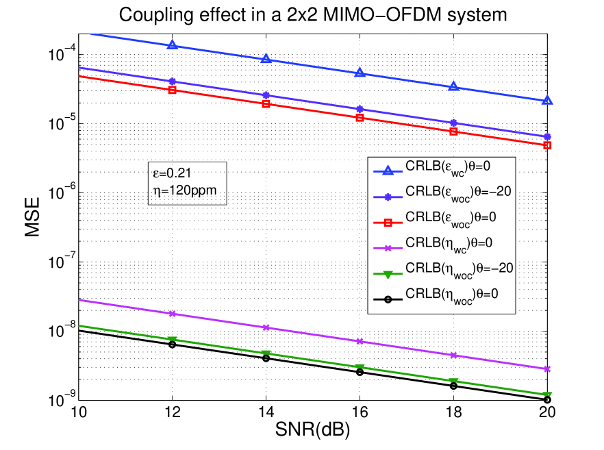
Figure 1: CRLB for the estimation of $\epsilon$ and $\eta$ as a function of SNR(dB) showing the coupling effect.

For the above given simulation setup, the change in CRLBs plotted in Fig.1 can be approximately represented as,

$$\mathrm{SNR}\hskip 2.84544pt\mathrm{at}\hskip 2.84544pt\mathrm{CRLB}(\epsilon_{wc})|_{\theta=0}\approx\mathrm{SNR}\hskip 2.84544pt\mathrm{at}\hskip 2.84544pt\mathrm{CRLB}(\epsilon_{woc})|_{\theta=0}+6.25\hskip 2.84544pt\mathrm{dB}$$

$$\mathrm{SNR}\hskip 2.84544pt\mathrm{at}\hskip 2.84544pt\mathrm{CRLB}(\eta_{wc})|_{\theta=0}\approx\mathrm{SNR}\hskip 2.84544pt\mathrm{at}\hskip 2.84544pt\mathrm{CRLB}(\eta_{woc})|_{\theta=0}+4.5\hskip 2.84544pt\mathrm{dB}$$

$$\mathrm{SNR}\hskip 2.84544pt\mathrm{at}\hskip 2.84544pt\mathrm{CRLB}(\epsilon_{woc})|_{\theta=-20}\approx\mathrm{SNR}\hskip 2.84544pt\mathrm{at}\hskip 2.84544pt\mathrm{CRLB}(\epsilon_{woc})|_{\theta=0}+1.25\hskip 2.84544pt\mathrm{dB}$$

$$\mathrm{SNR}\hskip 2.84544pt\mathrm{at}\hskip 2.84544pt\mathrm{CRLB}(\eta_{woc})|_{\theta=-20}\approx\mathrm{SNR}\hskip 2.84544pt\mathrm{at}\hskip 2.84544pt\mathrm{CRLB}(\eta_{woc})|_{\theta=0}+1\hskip 2.84544pt\mathrm{dB}$$

The above expressions show the effect of coupling of channel and STE on the estimation of CFO and SFO, respectively. Due to the coupling effect, the estimation of parameters without considering all impairments together results in performance degradation.

IV Maximum Likelihood Estimation

The ML cost function [3], [19] of the parameters $\epsilon,\theta,\eta,$ and $\mathbf{h}$, obtained from (9) is,

$$\arg\max_{\epsilon,\eta,\theta,\mathbf{h}}P(\mathbf{r}|\epsilon,\theta,\eta,\mathbf{h})=\arg\max_{\epsilon,\eta,\theta,\mathbf{h}}\frac{1}{(\pi\sigma_{w}^{2})^{NN_{R}}}\exp\left\{\frac{-\parallel{\mathbf{r}-\mathbf{A}\mathbf{h}}\parallel^{2}_{2}}{\sigma_{w}^{2}}\right\}.$$

Computing the log-likelihood function and simplifying, we obtain an equivalent cost function,

$$\arg\min_{\epsilon,\eta,\theta,\mathbf{h}}J(\epsilon,\eta,\theta,\mathbf{h}|\mathbf{r})=\arg\min_{\epsilon,\eta,\theta,\mathbf{h}}(\mathbf{r}-\mathbf{A}\mathbf{h})^{H}(\mathbf{r}-\mathbf{A}\mathbf{h}).$$ (33)

The multi-dimensional minimization in (33) gives the estimate of the parameters, ${\epsilon},{\theta},{\eta}$, and $\mathbf{h}$, which is practically not feasible. With perfect channel knowledge at receiver, the optimization problem in (33) reduces to a three-dimensional minimization problem as $\displaystyle\arg\min_{\epsilon,\eta,\theta}J(\epsilon,\eta,\theta|\mathbf{r},\mathbf{h})$, which also turns out to be too complex for practical purposes. In this section, we propose an ML algorithm in which the multi-dimensional optimization problem in (33) is reduced to a two-dimensional and a one-dimensional grid search, by rearranging the system model. Also, we propose a low complexity MML algorithm, which involves multiple one-dimensional searches, by making an approximation. Further, SML algorithm using different existing algorithms, which estimate fewer number of parameters, is also proposed.

IV-A Proposed ML Algorithm

The system model in (9) can be rewritten as

$$\mathbf{r} =\left(\mathbf{I}_{N_{R}}\otimes\left(\mathbf{DF}_{1}\mathbf{GX(\mathbf{I}}_{N_{T}}\otimes\mathbf{F}_{2})\right)\right)\mathbf{{h}}+\mathbf{w}$$ (34)

$$=\left(\mathbf{I}_{N_{R}}\otimes\left(\mathbf{DF}_{1}\mathbf{GX(\mathbf{I}}_{N_{T}}\otimes\mathbf{F}_{2\theta_{max}})\right)\right)\mathbf{{h}}^{\prime}+\mathbf{w},$$ (35)

$$\mathrm{where}\hskip 5.69046pt [\mathbf{F}_{2\theta_{max}}]_{k,l}=\exp(-j2\pi lk/N),$$ (36)

$$\mathrm{and}\hskip 5.69046pt \mathbf{h}{}^{\prime}=[\mathbf{h}{}^{\prime{\hskip 1.42271pt}T}_{\hskip 1.42271pt1},\mathbf{h}{}^{\prime{\hskip 1.42271pt}T}_{\hskip 1.42271pt2},\ldots,\mathbf{h}{}^{\prime{\hskip 1.42271pt}T}_{\hskip 1.42271ptN_{R}}]^{T},$$ (37)

with $\mathbf{h}{}^{\prime{\hskip 1.42271pt}}_{\hskip 1.42271ptv}=[\mathbf{h}{}^{\prime{\hskip 1.42271pt}T}_{\hskip 1.42271pt1,v},\mathbf{h}{}^{\prime{\hskip 1.42271pt}T}_{\hskip 1.42271pt2,v},\ldots,\mathbf{h}{}^{\prime{\hskip 1.42271pt}T}_{\hskip 1.42271ptN_{T},v}]^{T}$, and $\mathbf{h}{}^{\prime{\hskip 1.42271pt}}_{\hskip 1.42271ptu,v}=[\mathbf{h}^{T}_{u,v}\hskip 5.69046pt\mathbf{0}^{T}_{\theta_{max}\times 1}]^{T}$ for $k=0,1,\ldots,N-1$ and $l=0,1,\ldots,(L+\theta_{max}-1)$. The system model in (35) can also be represented as,

$$\mathbf{r} =\left(\mathbf{I}_{N_{R}}\otimes\left(\mathbf{DF}_{1}\mathbf{X(\mathbf{I}}_{N_{T}}\otimes\mathbf{F}_{2\theta_{max}})\right)\right)\mathbf{{h}}_{\theta}+\mathbf{w}$$ (38)

$$=\mathbf{A}_{1}\mathbf{{h}}_{\theta}+\mathbf{w},$$ (39)

$$\mathrm{where}\hskip 5.69046pt \mathbf{A}_{1}=\mathbf{I}_{N_{R}}\otimes(\mathbf{DF}_{1}\mathbf{X(\mathbf{I}}_{N_{T}}\otimes\mathbf{F}_{2\theta_{max}})),$$ (40)

$$\mathrm{and}\hskip 5.69046pt \mathbf{h}_{\theta}=[\mathbf{h}_{1_{\theta}}^{T},\mathbf{h}_{2_{\theta}}^{T},\ldots,\mathbf{h}_{N_{R\theta}}^{T}]^{T},$$ (41)

with $\mathbf{h}_{v_{\theta}}=[\mathbf{h}_{(1,v)_{\theta}}^{T},\mathbf{h}_{(2,v)_{\theta}}^{T},\ldots,\mathbf{h}_{(N_{T},v)_{\theta}}^{T}]^{T}$, and $\mathbf{h}_{(u,v)_{\theta}}=[\mathbf{0}^{T}_{\theta\times 1}\hskip 5.69046pt\mathbf{h}_{u,v}^{T}\hskip 5.69046pt\mathbf{0}^{T}_{(\theta_{max}-\theta)\times 1}]^{T}$,
for $u=0,1,\ldots,N_{T}-1,$ and $v=0,1,\ldots,N_{R}-1$. From (39), the least squares estimate of $\mathbf{{h}}_{\theta}$ is given by, $\hat{\mathbf{{h}}}_{\theta}={\mathbf{A}^{{\dagger}}_{1}}\mathbf{r}$. Let $\mathbf{P{}_{A_{1}}}$ be the projection matrix of $\mathbf{A}_{1}$. Therefore, the estimate of $\epsilon$ and $\eta$ can be obtained from (39) as,

$$\displaystyle[\hat{\epsilon}_{ML},\hat{\eta}_{ML}] =\arg\min_{\epsilon,\eta}(\mathbf{r}-\mathbf{A}_{1}\mathbf{A}^{{\dagger}}_{1}\mathbf{r})^{H}(\mathbf{r}-\mathbf{A}_{1}\mathbf{A}^{{\dagger}}_{1}\mathbf{r})$$ (42)

$$=\arg\max_{\epsilon,\eta}\parallel\mathbf{P{}_{A_{1}}}\mathbf{r}\parallel_{2}^{2}$$ (43)

$$=\arg\max_{\epsilon,\eta}J_{1}(\epsilon,\eta|\mathbf{r})$$

$$\mathrm{where}\hskip 5.69046ptJ_{1}(\epsilon,\eta|\mathbf{r})=\parallel\mathbf{P{}_{A_{1}}}\mathbf{r}\parallel_{2}^{2}.$$ (44)

From (9), the least squares estimate of $\mathbf{{h}}$ is given by, $\hat{\mathbf{{h}}}={\mathbf{A}^{{\dagger}}}\mathbf{r}$. Let $\mathbf{P{}_{A}}$ be the projection matrix of $\mathbf{A}$. Therefore, using the estimates of $\epsilon$ and $\eta$ from (43), the estimate of $\theta$ can be obtained as,

$$\displaystyle[\hat{\theta}_{ML}] =\arg\min_{\theta}(\mathbf{r}-\mathbf{A}\mathbf{A}^{{\dagger}}\mathbf{r})^{H}(\mathbf{r}-\mathbf{A}\mathbf{A}^{{\dagger}}\mathbf{r})$$ (45)

$$=\arg\max_{\theta}\parallel\mathbf{P{}_{A}}\mathbf{r}\parallel_{2}^{2}$$ (46)

$$=\arg\max_{\theta}J_{2}(\theta|\mathbf{r},\hat{\epsilon}_{ML},\hat{\eta}_{ML})$$

$$\mathrm{where}\hskip 5.69046ptJ_{2}(\theta|\mathbf{r},\hat{\epsilon}_{ML},\hat{\eta}_{ML})=\parallel\mathbf{P{}_{A}}\mathbf{r}\parallel_{2}^{2}.$$ (47)

Finally, using the estimates of $\epsilon$, $\eta$, and $\theta$, we get the estimate of $\mathbf{h}$ as,

$$[\hat{\mathbf{h}}_{ML}]=\hat{\mathbf{A}}^{\dagger}\mathbf{r}$$ (48)

$$\mathrm{where}\hskip 5.69046pt\hat{\mathbf{A}}=\mathbf{I}_{N_{R}}\otimes\left(\mathbf{D}(\hat{\epsilon}_{ML},\hat{\eta}_{ML})\mathbf{F}_{1}(\hat{\eta}_{ML})\mathbf{G}(\hat{\theta}_{ML})\mathbf{X}\left(\mathbf{I}_{N_{T}}\otimes\mathbf{F}_{2}\right)\right).$$ (49)

The series of steps involved are given in Algorithm $1$.

Algorithm 1 ML Algorithm

Inputs: $N$, $N_{T}$, $N_{R}$, $\mathbf{r}$, $\mathbf{X}$, $L_{m}$, $[\theta_{min},\theta_{max},\theta_{grid}]$, $[\epsilon_{min},\epsilon_{max},\epsilon_{grid}]$, $[\eta_{min},\eta_{max},\eta_{grid}]$

1:  Evaluate $\mathbf{F}_{2}$, $\mathbf{F}_{2\theta_{max}}$;$\star$ using (4), (36)

2:  for $i=$ $\epsilon_{min}:\epsilon_{grid}:\epsilon_{max}$ do

3:     for $j=$ $\eta_{min}:\eta_{grid}:\eta_{max}$ do

4:        Evaluate $\mathbf{D}(i,j)$, $\mathbf{F}_{1}(j)$;$\star$ using (6), (3)

5:        $\mathbf{A}_{1}(i,j)=\mathbf{I}_{N_{R}}\otimes\left(\mathbf{D}(i,j)\mathbf{F}_{1}(j)\mathbf{X}(\mathbf{I}_{N_{T}}\otimes\mathbf{F}_{2\theta_{max}})\right)$ ;$\star$ using (40)

6:        $J_{1}(i,j|\mathbf{r})=\parallel\mathbf{P{}_{A_{1}}}\mathbf{r}\parallel_{2}^{2}$;$\star$ using (44)

7:     end for

8:  end for

9:  $\displaystyle[\hat{\epsilon}_{ML},\hat{\eta}_{ML}]=\arg\max_{i,j}J_{1}(i,j|\mathbf{r})$;

10:  Evaluate $\mathbf{D}(\hat{\epsilon}_{ML},\hat{\eta}_{ML})$, $\mathbf{F}_{1}(\hat{\eta}_{ML})$;$\star$ using (6), (3)

11:  for $k=$ $\theta_{min}:\theta_{grid}:\theta_{max}$ do

12:     Evaluate $\mathbf{G}(k)$, $\mathbf{A}(\hat{\epsilon}_{ML},\hat{\eta}_{ML},k)$;$\star$ using (7), (10)

13:     $J_{2}(k|\mathbf{r},\hat{\epsilon}_{ML},\hat{\eta}_{ML})=\parallel\mathbf{P{}_{A}}\mathbf{r}\parallel_{2}^{2}$;$\star$ using (47)

14:  end for

15:  $\displaystyle[\hat{\theta}_{ML}]=\arg\max_{k}J_{2}(k|\mathbf{r},\hat{\epsilon}_{ML},\hat{\eta}_{ML})$;

16:  Evaluate $\mathbf{G}(\hat{\theta}_{ML})$;$\star$ using (7)

17:  $\hat{\mathbf{A}}=\mathbf{I}_{N_{R}}\otimes\left(\mathbf{D}(\hat{\epsilon}_{ML},\hat{\eta}_{ML})\mathbf{F}_{1}(\hat{\eta}_{ML})\mathbf{G}(\hat{\theta}_{ML})\mathbf{X}(\mathbf{I}_{N_{T}}\otimes\mathbf{F}_{2})\right)$;$\star$ using (49)

18:  $[\hat{\mathbf{h}}_{ML}]=\hat{\mathbf{A}}^{\dagger}\mathbf{r}$;$\star$ using (48)

Output: $[\hat{\theta}_{ML},\hat{\epsilon}_{ML},\hat{\eta}_{ML},\hat{\mathbf{h}}_{ML}]$

IV-B Proposed Modified ML (MML) Algorithm

Algorithm 2 MML Algorithm

Inputs: $N$, $N_{T}$, $N_{R}$, $\mathbf{r}$, $\mathbf{X}$, $L_{m}$, $[\theta_{min},\theta_{max},\theta_{grid}]$, $[\eta_{min},\eta_{max},\eta_{grid}]$

1:  Evaluate $\mathbf{F}_{2}$, $\mathbf{F}_{2\theta_{max}}$, $\mathbf{C}_{1}$;$\star$ using (4), (36), (14)

2:  $\mathbf{R}=diag(\mathbf{r})$;

3:  for $j=$ $\eta_{min}:\eta_{grid}:\eta_{max}$ do

4:     Evaluate $\mathbf{F}_{1}(j)$, $\mathbf{A}_{2}(j)$;$\star$ using (3), (51)

5:     $\mathbf{C}=\mathbf{R}^{H}\left(\mathbf{I}_{NN_{R}}-\left(\mathbf{I}_{N_{R}}\otimes\mathbf{P{}_{A_{2}}}\right)\right)$;$\star$ using (54)

6:     $\mathbf{c}_{1}(j)=\displaystyle\frac{2\pi(1+j)}{N}diag(\mathbf{I}_{N_{R}}\otimes\mathbf{C}_{1})$;$\star$ using (55)

7:     $\hat{\epsilon}(j)=\displaystyle\frac{\mathbf{c}^{T}_{1}\Im(\mathbf{C}\mathbf{C}^{H})\mathbf{1}}{\mathbf{c}^{T}_{1}\Re(\mathbf{C}\mathbf{C}^{H})\mathbf{c}_{1}}$;$\star$ using (57)

8:     Evaluate $J_{3}(j|\mathbf{r})$;$\star$ using (58)

9:  end for

10:  $\displaystyle[\hat{\eta}_{MML}]=\arg\min_{j}J_{3}(j|\mathbf{r})$;$\star$ using (59)

11:  $[\hat{\epsilon}_{MML}]=\hat{\epsilon}(\hat{\eta}_{MML})$;$\star$ evaluation similar to step 7

12:  Evaluate $\mathbf{D}(\hat{\epsilon}_{MML},\hat{\eta}_{MML})$, $\mathbf{F}_{1}(\hat{\eta}_{MML})$;$\star$ using (6), (3)

13:  Remaining steps are same as steps from $11$ to $18$ in Algorithm $1$.

Output: $[\hat{\theta}_{MML},\hat{\epsilon}_{MML},\hat{\eta}_{MML},\hat{\mathbf{h}}_{MML}]$

The estimation of $\epsilon$ and $\eta$, using (43), by a two dimensional grid search is not desirable for practical applications. Hence, a reduced complexity MML algorithm is obtained in this section. From (40), we have

$$\mathbf{A}_{1} =\mathbf{I}_{N_{R}}\otimes(\mathbf{DF_{1}X(\mathbf{I}}_{N_{T}}\otimes\mathbf{F}_{2\theta_{max}}))$$

$$=\mathbf{I}_{N_{R}}\otimes\mathbf{D}\mathbf{A}_{2},$$ (50)

$$\mathrm{where}\hskip 14.22636pt \mathbf{A}_{2}=\mathbf{F}_{1}\mathbf{X(\mathbf{I}}_{N_{T}}\otimes\mathbf{F}_{2\theta_{max}}).$$ (51)

Therefore, from (38), (40), and (IV-B), the least squares estimate of $\mathbf{{h}}_{\theta}$ is given by,

$$\hat{\mathbf{{h}}}_{\theta} ={\mathbf{A}^{{\dagger}}_{1}}\mathbf{r}$$

$$=(\mathbf{A}^{H}_{1}\mathbf{A}_{1})^{-1}\mathbf{A}^{H}_{1}\mathbf{r}$$

$$=\left(\mathbf{I}_{N_{R}}\otimes\left((\mathbf{A}^{H}_{2}\mathbf{A}_{2})^{-1}\mathbf{A}^{H}_{2}\mathbf{D}^{H}\right)\right)\mathbf{r}.$$ (52)

Using (IV-B) and (52), the cost function of the two dimensional grid search in (42) can be written as,

$$( \mathbf{r}-\mathbf{A}_{1}\mathbf{A}^{{\dagger}}_{1}\mathbf{r})^{H}(\mathbf{r}-\mathbf{A}_{1}\mathbf{A}^{{\dagger}}_{1}\mathbf{r})$$

$$=\left(\mathbf{r}-\left(\mathbf{I}_{N_{R}}\otimes\left(\mathbf{D}\mathbf{A}_{2}(\mathbf{A}^{H}_{2}\mathbf{A}_{2})^{-1}\mathbf{A}^{H}_{2}\mathbf{D}^{H}\right)\right)\mathbf{r}\right)^{H}\left(\mathbf{r}-\left(\mathbf{I}_{N_{R}}\otimes\left(\mathbf{D}\mathbf{A}_{2}(\mathbf{A}^{H}_{2}\mathbf{A}_{2})^{-1}\mathbf{A}^{H}_{2}\mathbf{D}^{H}\right)\right)\mathbf{r}\right)$$

$$=\mathbf{r}^{H}(\mathbf{I}_{N_{R}}\otimes\mathbf{D})\left(\mathbf{I}_{NN_{R}}-\left(\mathbf{I}_{N_{R}}\otimes\mathbf{P{}_{A_{2}}}\right)\right)\left(\mathbf{I}_{NN_{R}}-\left(\mathbf{I}_{N_{R}}\otimes\mathbf{P{}_{A_{2}}}\right)\right)(\mathbf{I}_{N_{R}}\otimes\mathbf{D}^{H})\mathbf{r}$$

$$=\mathbf{d}^{T}\mathbf{R}^{H}\left(\mathbf{I}_{NN_{R}}-\left(\mathbf{I}_{N_{R}}\otimes\mathbf{P{}_{A_{2}}}\right)\right)\left(\mathbf{I}_{NN_{R}}-\left(\mathbf{I}_{N_{R}}\otimes\mathbf{P{}_{A_{2}}}\right)\right)\mathbf{R}\mathbf{d^{*}}$$

$$=\mathbf{d}^{T}\mathbf{C}\mathbf{C}^{H}\mathbf{d^{*}}$$ (53)

$$\mathrm{where}\hskip 5.69046pt\mathbf{R}=diag(\mathbf{r}),\mathbf{d}=diag(\mathbf{I}_{N_{R}}\otimes\mathbf{D}),\mathbf{D}^{H}\mathbf{D}=\mathbf{D}\mathbf{D}^{H}=\mathbf{I}_{N},\mathbf{P{}_{A_{2}}}=\mathbf{A}_{2}(\mathbf{A}^{H}_{2}\mathbf{A}_{2})^{-1}\mathbf{A}^{H}_{2},\hskip 2.84544pt\mathrm{and}\hskip 5.69046pt$$

$$\mathbf{C}=\mathbf{R}^{H}\left(\mathbf{I}_{NN_{R}}-\left(\mathbf{I}_{N_{R}}\otimes\mathbf{P{}_{A_{2}}}\right)\right).$$ (54)

For small values of $\epsilon$, $\mathbf{d}\approx\mathbf{1}+j\epsilon\mathbf{c}_{1}$, where

$$\mathbf{c}_{1}=\displaystyle\frac{2\pi(1+\eta)}{N}diag(\mathbf{I}_{N_{R}}\otimes\mathbf{C}_{1})$$ (55)

with $\mathbf{C}_{1}$ as given in (14). Therefore, (53) can be written as,

$$\mathbf{d}^{T}\mathbf{C} \mathbf{C}^{H}\mathbf{d^{*}}\approx[\mathbf{1}+j\epsilon\mathbf{c}_{1}]^{T}\mathbf{C}\mathbf{C}^{H}[\mathbf{1}-j\epsilon\mathbf{c}_{1}]$$

$$=\mathbf{1}^{T}\mathbf{C}\mathbf{C}^{H}\mathbf{1}+j\epsilon\mathbf{c}_{1}^{T}\mathbf{C}\mathbf{C}^{H}\mathbf{1}-j\epsilon\mathbf{1}^{T}\mathbf{C}\mathbf{C}^{H}\mathbf{c}_{1}+\epsilon^{2}\mathbf{c}^{T}_{1}\mathbf{C}\mathbf{C}^{H}\mathbf{c}_{1}$$

$$=\mathbf{1}^{T}\mathbf{C}\mathbf{C}^{H}\mathbf{1}+\epsilon^{2}\mathbf{c}_{1}^{T}\Re(\mathbf{C}\mathbf{C}^{H})\mathbf{c}_{1}-2\epsilon\mathbf{c}_{1}^{T}\Im(\mathbf{C}\mathbf{C}^{H})\mathbf{1}$$ (56)

Differentiating (56) with respect to $\epsilon$ and equating to ${0}$ gives the estimate of $\epsilon$ in terms of $\eta$ as,

$$\hat{\epsilon}=\displaystyle\frac{\mathbf{c}^{T}_{1}\Im(\mathbf{C}\mathbf{C}^{H})\mathbf{1}}{\mathbf{c}^{T}_{1}\Re(\mathbf{C}\mathbf{C}^{H})\mathbf{c}_{1}}$$ (57)

Substituting (57) into (56), we have

$$J_{3}(\eta|\mathbf{r})=\mathbf{1}^{T}\mathbf{C}\mathbf{C}^{H}\mathbf{1}+\hat{\epsilon}^{2}\mathbf{c}_{1}^{T}\Re(\mathbf{C}\mathbf{C}^{H})\mathbf{c}_{1}-2\hat{\epsilon}\mathbf{c}_{1}^{T}\Im(\mathbf{C}\mathbf{C}^{H})\mathbf{1}.$$ (58)

Using (58), we get the estimate of $\eta$ by MML algorithm as

$$[\hat{\eta}_{MML}]=\arg\min_{\eta}J_{3}(\eta|\mathbf{r}).$$ (59)

Substituting (59) into (57) gives the estimate of $\epsilon$. Using the estimates of $\epsilon$ and $\eta$, the estimates of $\theta$ and $\mathbf{h}$ can be obtained using (47) and (48), as done in Algorithm $1$. The series of steps involved are given in Algorithm $2$.

Remarks

For the range of values of $|\epsilon|$ less than $0.10$, the equation (56) holds reasonably good with average error of the approximation less than $10^{-4}$.

IV-C Proposed Stage-wise ML (SML) Algorithm

We also propose SML algorithm in which the joint estimation of CFO and STE is done in the first stage using the algorithm in [6], ignoring the effect of SFO. Using the system model in (9) and ignoring $\eta$, we have

$$\mathbf{A}(\epsilon,0,\theta)=\mathbf{I}_{N_{R}}\otimes(\mathbf{D}(\epsilon,0)\mathbf{F}_{1}(0)\mathbf{G}(\theta)\mathbf{X(\mathbf{I}}_{N_{T}}\otimes\mathbf{F_{2}}))$$ (60)

$$\mathrm{and}\hskip 14.22636pt[\hat{\epsilon}_{SML},\hat{\theta}_{SML}] =\arg\min_{\epsilon,\theta}(\mathbf{r}-\mathbf{A}\mathbf{A}^{{\dagger}}\mathbf{r})^{H}(\mathbf{r}-\mathbf{A}\mathbf{A}^{{\dagger}}\mathbf{r})$$

$$=\arg\max_{\epsilon,\theta}\parallel\mathbf{P{}_{A}}\mathbf{r}\parallel_{2}^{2}$$ (61)

$$=\arg\max_{\epsilon,\theta}J_{4}(\epsilon,\theta|\mathbf{r})$$

$$\mathrm{where}\hskip 5.69046ptJ_{4}(\epsilon,\eta|\mathbf{r}) =\parallel\mathbf{P{}_{A}}\mathbf{r}\parallel_{2}^{2}.$$ (62)

With the estimates of CFO and STE from (61) in the first stage, the received signal is used to estimate SFO and channel using the ML algorithm in [8], as extended to a MIMO-OFDM system, in the second stage.

$$\displaystyle[\hat{\eta}_{SML}] =\arg\min_{\eta}(\mathbf{r}-\mathbf{A}\mathbf{A}^{{\dagger}}\mathbf{r})^{H}(\mathbf{r}-\mathbf{A}\mathbf{A}^{{\dagger}}\mathbf{r})$$

$$=\arg\max_{\eta}\parallel\mathbf{P{}_{A}}\mathbf{r}\parallel_{2}^{2}$$ (63)

$$=\arg\max_{\eta}J_{5}(\eta|\mathbf{r},\hat{\epsilon}_{SML},\hat{\theta}_{SML})$$

$$\mathrm{where}\hskip 5.69046ptJ_{5}(\eta|\mathbf{r},\hat{\epsilon}_{SML},\hat{\theta}_{SML})=\parallel\mathbf{P{}_{A}}\mathbf{r}\parallel_{2}^{2}.$$ (64)

Finally, using the estimates of $\epsilon$, $\eta$, and $\theta$, we get the estimate of $\mathbf{h}$ as in (48). The series of steps involved are given in Algorithm $3$.

Algorithm 3 SML Algorithm

Inputs: $N$, $N_{T}$, $N_{R}$, $\mathbf{r}$, $\mathbf{X}$, $L_{m}$, $[\theta_{min},\theta_{max},\theta_{grid}]$, $[\epsilon_{min},\epsilon_{max},\epsilon_{grid}]$, $[\eta_{min},\eta_{max},\eta_{grid}]$

1:  Evaluate $\mathbf{F}_{2}$, $\mathbf{F}_{1}(0)$;$\star$ using (4), (3) and $\eta$ is ignored

2:  for $i=$ $\epsilon_{min}:\epsilon_{grid}:\epsilon_{max}$ do

3:     for $k=$ $\theta_{min}:\theta_{grid}:\theta_{max}$ do

4:        Evaluate $\mathbf{D}(i,0)$, $\mathbf{G}(k)$;$\star$ using (6), (7) and $\eta$ is ignored

5:        $\mathbf{A}(i,0,k)=\mathbf{I}_{N_{R}}\otimes\left(\mathbf{D}(i,0)\mathbf{F}_{1}(0)\mathbf{G}(k)\mathbf{X}(\mathbf{I}_{N_{T}}\otimes\mathbf{F}_{2})\right)$ ;$\star$ using (60)

6:        $J_{4}(i,k|\mathbf{r})=\parallel\mathbf{P{}_{A}}\mathbf{r}\parallel_{2}^{2}$;$\star$ using (62)

7:     end for

8:  end for

9:  $\displaystyle[\hat{\epsilon}_{SML},\hat{\theta}_{SML}]=\arg\max_{i,k}J_{4}(i,k|\mathbf{r})$;

10:  Evaluate $\mathbf{G}(\hat{\theta}_{SML})$;$\star$ using (7)

11:  for $j=$ $\eta_{min}:\eta_{grid}:\eta_{max}$ do

12:     Evaluate $\mathbf{D}(\hat{\epsilon}_{SML},j)$, $\mathbf{F}_{1}(j)$, $\mathbf{A}(\hat{\epsilon}_{SML},j,\hat{\theta}_{SML})$;$\star$ using (6), (3), (10)

13:     $J_{5}(j|\mathbf{r},\hat{\epsilon}_{SML},\hat{\theta}_{SML})=\parallel\mathbf{P{}_{A}}\mathbf{r}\parallel_{2}^{2}$;$\star$ using (64)

14:  end for

15:  $\displaystyle[\hat{\eta}_{SML}]=\arg\max_{k}J_{5}(j|\mathbf{r},\hat{\epsilon}_{SML},\hat{\theta}_{SML})$;

16:  $\hat{\mathbf{A}}(\hat{\epsilon}_{SML},\hat{\eta}_{SML},\hat{\theta}_{SML})$;$\star$ using (10)

17:  $[\hat{\mathbf{h}}_{SML}]=\hat{\mathbf{A}}^{\dagger}\mathbf{r}$;$\star$ using (48)

Output: $[\hat{\theta}_{SML},\hat{\epsilon}_{SML},\hat{\eta}_{SML},\hat{\mathbf{h}}_{SML}]$

IV-D Comparison of Computational Complexity

The computational complexity of ML algorithm depends mainly on computation of the two-dimensional grid search in (43), for obtaining the estimates of $\epsilon$ and $\eta$, and the one-dimensional grid search in (46), for obtaining the estimate of $\theta$. Let $g_{\epsilon}$, $g_{\eta}$, and $g_{\theta}$ denote the number of grid points used in search for $\epsilon$, $\eta$, and $\theta$. Therefore, the computational complexity of evaluating (43) is approximately equal to $g_{\epsilon}g_{\eta}\mathcal{O}(N^{3})$, whereas that of evaluating (46) is approximately equal to $g_{\theta}\mathcal{O}(N^{3})$. Thus, the total computational complexity of ML algorithm is approximately given by $(g_{\epsilon}g_{\eta}+g_{\theta})\mathcal{O}(N^{3})$.

The computational complexity of MML algorithm depends mainly on the computation of two one-dimensional grid searches, given in (59) and (46). The computational complexity of evaluating (59) is approximately equal to $g_{\eta}\mathcal{O}(N^{3})$, whereas that of evaluating (46) is approximately equal to $g_{\theta}\mathcal{O}(N^{3})$. Thus, the total computational complexity of MML algorithm is approximately given by $(g_{\eta}+g_{\theta})\mathcal{O}(N^{3})$.

The computational complexity of SML algorithm depends mainly on the computation of the two-dimensional grid search in (61), for the estimation of $\epsilon$ and $\theta$ in the first stage, and the one-dimensional grid search in (63), for the estimation of $\eta$ in the second stage. The total computational complexity of the first stage is approximately equal to $g_{\epsilon}g_{\theta}\mathcal{O}(N^{3})$, whereas that of second stage is approximately equal to $g_{\eta}\mathcal{O}(N^{3})$. Thus, the total computational complexity of SML algorithm is approximately given by $(g_{\epsilon}g_{\theta}+g_{\eta})\mathcal{O}(N^{3})$.

Remarks

Based on the system setup in Section V, the typical values of $g_{\epsilon}$, $g_{\eta}$, and $g_{\theta}$ are $81$, $101$, and $43$, respectively. Thus, MML algorithm is around 57 times and 25 times faster than ML and SML algorithms, respectively.

V Simulation Results and Discussions

V-A System Setup

The simulated $2\times 2$ MIMO-OFDM system has $N=128$ subcarriers for each transmitter with $20$ MHz signal bandwidth. The SCM specified by 3GPP [21], is used to generate the fading channels in the Urban Macro Scenario with $L_{m}=10$. Also, The transmitted symbols belong to QPSK constellation with unit amplitude. Therefore, the variance of the complex additive Gaussian noise at the receiver, $\sigma^{2}_{w}$, is varied for getting SNR(dB) in steps of $5$ for the evaluation of Mean Square Error (MSE) and CRLB. Also, $10^{3}$ trials are carried out in simulations for getting each point in the MSE and CRLB plots.

We consider the training blocks having a CP of length $32$. The condition $(L_{m}+\theta_{max})$ less than length of CP results in $\theta_{max}=21$ and $|\theta|<21$. The range of normalized CFO used for grid search is $|\epsilon|<0.4$ with a resolution of $10^{-2}$ and that of normalized SFO is $|\eta|<5\times 10^{-3}$ with a resolution of $10^{-4}$. The actual values of the impairments, $\epsilon$, $\eta$, and $\theta$ used in the simulations are $0.021$, $0.000101$ or $101$ $\mathrm{ppm}$, and $2$, respectively.

V-B Performance Measures

The ML estimates of the parameters are used for calculating the MSE values as,

$$\mathrm{MSE}(\hat{\boldsymbol{\rho}})=\frac{\sum\limits_{i=1}^{N_{trials}}\parallel\hat{\boldsymbol{\rho}}_{i}-\boldsymbol{\rho}\parallel^{2}_{2}}{N_{trials}}.$$ (65)

where $\boldsymbol{\rho}$ represents the actual parameter, $\hat{\boldsymbol{\rho}}_{i}$ represents the estimate of the parameter at $i^{\mathrm{th}}$ trial, and $N_{trials}$ represents the number of trials. The Probability of Timing Failure $(P_{tf})$ is used as an indicator to illustrate the robustness of symbol timing estimator [7], which is expressed as,

$$P_{tf}(p)=Pr\left[|\hat{\theta}-\theta|\geqslant p\right]$$ (66)

where $p$ is the absolute difference between the estimated value of $\theta$ and the actual value of $\theta$.

V-C Performance Assessment

The MSE values of the estimated parameters are calculated using (65) and are plotted in log-scale against SNR(dB) for ML, MML, and SML algorithms in Fig.$2$-Fig.$5$. The CRLBs of the parameters are also plotted in the corresponding figures.

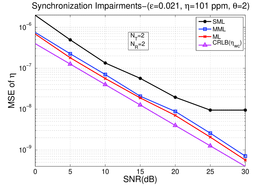
Figure 2: CRLB and MSE for the estimation of SFO as a function of SNR(dB) using ML, MML, and SML algorithms.

It is found from Fig.2 and Fig.3 that the MSE plots of the ML algorithm for the estimation of $\eta$ and $\epsilon$ closely follows $\mathrm{CRLB}(\eta_{wc})$ and $\mathrm{CRLB}(\epsilon_{wc})$, but with a performance degradation of around $1.25$ dB SNR and $0.75$ dB SNR, respectively. Also, it is found that there is only small performance difference between ML and MML algorithms. Performance loss of more than $3$dB, and error floor at $25$ dB occurs for SML algorithm when compared with the performance of ML or MML algorithms in Fig.2 and Fig.3, respectively.

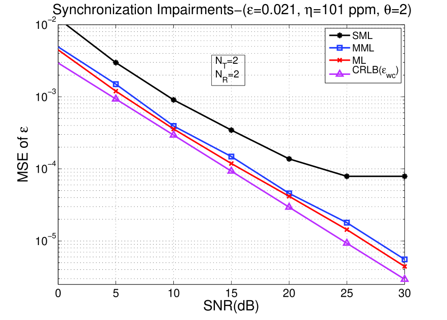
Figure 3: CRLB and MSE for the estimation of CFO as a function of SNR(dB) using ML, MML, and SML algorithms.

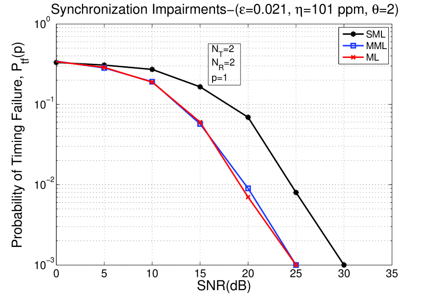
Figure 4: Probability of Timing Failure as a function of SNR(dB) using ML, MML, and SML algorithms.

The probability of timing failure for the estimation of $\theta$ is calculated for $p=1$, as defined in (66), and is plotted in Fig.4 for ML, MML, and SML algorithms, respectively. As in the cases of $\epsilon$ and $\eta$, there is only small performance degradation due to the approximation in the MML algorithm, and performance loss of more than $3$dB occurs for SML algorithm when compared with ML algorithm, as observed from the plots in Fig.4.

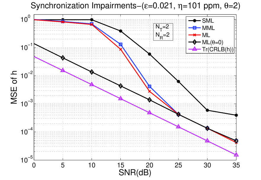
Figure 5: CRLB and MSE for the estimation of channel as a function of SNR(dB) using ML, MML, and SML algorithms.

The MSE plots of ML estimates of $\mathbf{h}$ using ML algorithm with STE=0, denoted as ML($\theta=0$), together with ML, MML, and SML algorithms are shown in Fig.5. Tr($\mathrm{CRLB}$($\mathbf{h}$)) evaluated using (32) is also shown in the same figure. It is found from Fig.5 that MSE plot of ML($\theta=0$) follows Tr($\mathrm{CRLB}(\mathbf{h})$) with a performance loss of $4$ dB. Comparing the MSE plots of ML($\theta=0$) and ML in the figure, it is found that the performance degradation of ML algorithm below $20$ dB SNR is due to the coupling effect of STE on the channel. As in the cases of $\epsilon$, $\eta$ and $\theta$, there is only small performance degradation due to the approximation in the MML algorithm. Also, the performance degradation and error floor of the MSE plot of SML algorithm is due to the stage-wise estimation of the parameters.

Thus, it is found from the figures that there is only small performance degradation due to the approximation in the MML algorithm when compared with ML algorithm. Also, performance degradation occurs, if joint estimation of all impairments together is not done, as observed from the performance plots of SML algorithm in the figures.

VI Conclusion

In this paper, ML algorithms, for the joint estimation of synchronization impairments and channel in a MIMO-OFDM system, are proposed. A system model, which shows the effects of the synchronization impairments and channel, is formulated. CRLBs for the estimation of continuous parameters are derived, which show the coupling effect among different parameters and the significance of a joint estimator. An ML estimation algorithm is proposed, where the multi-dimensional optimization problem for estimating the parameters is reduced to a two-dimensional and a one-dimensional grid search. To reduce the complexity further, MML algorithm which involves only multiple one-dimensional searches is also proposed. Further, SML algorithm using existing algorithms, which estimate fewer number of parameters, is also proposed. The performances of the estimation methods are studied through numerical simulations and it is observed that, there is only small performance degradation due to the approximation in MML algorithm. Also, the proposed ML and MML algorithms exhibit better performance than the proposed SML algorithm, which uses existing algorithms.

References

• [1] M. Speth, S. Fechtel, G. Fock, and H. Meyr, “Optimum receiver design for wireless broad-band systems using ofdm. 1,” IEEE Trans. Commun., vol. 47, pp. 1668 –1677, Nov 1999.
• [2] M. Morelli, C.-C. Kuo, and M.-O. Pun, “Synchronization techniques for orthogonal frequency division multiple access (ofdma): A tutorial review,” Proceedings of the IEEE, vol. 95, pp. 1394 –1427, july 2007.
• [3] M.-O. Pun, M. Morelli, and C.-C. Kuo, “Maximum-likelihood synchronization and channel estimation for ofdma uplink transmissions,” IEEE Trans. Commun., vol. 54, pp. 726 – 736, april 2006.
• [4] H. Nguyen-Le, T. Le-Ngoc, and C. C. Ko, “Joint channel estimation and synchronization for mimo ofdm in the presence of carrier and sampling frequency offsets,” IEEE Trans. Vehicular Technol., vol. 58, pp. 3075 –3081, july 2009.
• [5] J.-W. Choi, J. Lee, Q. Zhao, and H.-L. Lou, “Joint ml estimation of frame timing and carrier frequency offset for ofdm systems employing time-domain repeated preamble,” IEEE Trans. Wireless Commun., vol. 9, pp. 311 –317, january 2010.
• [6] S. Salari and M. Heydarzadeh, “Joint maximum-likelihood estimation of frequency offset and channel coefficients in multiple-input multiple-output orthogonal frequency-division multiplexing systems with timing ambiguity,” IET Commun., vol. 5, pp. 1964 –1970, 23 2011.
• [7] A. Saemi, V. Meghdadi, J.-P. Cances, and M. Zahabi, “Joint ml time-frequency synchronisation and channel estimation algorithm for mimo-ofdm systems,” IET Circuits Devices Syst., vol. 2, pp. 103 –111, february 2008.
• [8] S. Gault, W. Hachem, and P. Ciblat, “Joint sampling clock offset and channel estimation for ofdm signals: Cramer-rao bound and algorithms,” IEEE Trans. Signal Process., vol. 54, pp. 1875 – 1885, may 2006.
• [9] Y.-H. Kim and J.-H. Lee, “Joint maximum likelihood estimation of carrier and sampling frequency offsets for ofdm systems,” IEEE Trans. Broadcast., vol. 57, pp. 277 –283, june 2011.
• [10] R. Jose and K. V. S. Hari, “Joint estimation of synchronization impairments in mimo-ofdm system,” in 2012 National Conference on Communications (NCC), pp. 1 –5, feb. 2012.
• [11] T. Schmidl and D. Cox, “Robust frequency and timing synchronization for ofdm,” IEEE Trans. Commun., vol. 45, pp. 1613 –1621, dec 1997.
• [12] H. Minn, V. Bhargava, and K. Letaief, “A robust timing and frequency synchronization for ofdm systems,” IEEE Trans. Wireless Commun., vol. 2, pp. 822 – 839, july 2003.
• [13] K. Shi and E. Serpedin, “Coarse frame and carrier synchronization of ofdm systems: a new metric and comparison,” IEEE Trans. Wireless Commun., vol. 3, pp. 1271 – 1284, july 2004.
• [14] M. Morelli, “Timing and frequency synchronization for the uplink of an ofdma system,” IEEE Trans. Commun., vol. 52, p. 166, jan. 2004.
• [15] T. Lv, H. Li, and J. Chen, “Joint estimation of symbol timing and carrier frequency offset of ofdm signals over fast time-varying multipath channels,” IEEE Trans. Signal Process., vol. 53, pp. 4526 – 4535, dec. 2005.
• [16] P. Stoica and O. Besson, “Training sequence design for frequency offset and frequency-selective channel estimation,” IEEE Trans. Commun., vol. 51, pp. 1910 – 1917, nov. 2003.
• [17] M. Morelli and U. Mengali, “Carrier-frequency estimation for transmissions over selective channels,” IEEE Trans. Commun., vol. 48, pp. 1580 –1589, sep 2000.
• [18] H. Nguyen-Le, T. Le-Ngoc, and C. C. Ko, “Rls-based joint estimation and tracking of channel response, sampling, and carrier frequency offsets for ofdm,” IEEE Trans. Broadcast., vol. 55, pp. 84 –94, march 2009.
• [19] S. M. Kay, Fundamentals of statistical signal processing: estimation theory. Upper Saddle River, NJ, USA: Prentice-Hall, Inc., 1993.
• [20] R. A. Horn and C. R. Johnson, Matrix Analysis. Cambridge University Press, 1990.
• [21] “Spatial channel model for multiple input multiple output (mimo) simulations,” 3GPP, vol. TR 25.996, no. v6.1.0, Sep. 2003.