Extrinsic spin Nernst effect in two-dimensional electron systems

Abstract

The spin accumulation due to the spin current induced by the perpendicular temperature gradient (the spin Nernst effect) is studied in a two-dimensional electron system (2DES) with spin-orbit interaction by employing the Boltzmann equation. The considered 2DES is confined within a symmetric quantum well with delta doping at the center of the well. A symmetry consideration leads to the spin-orbit interaction which is diagonal in the spin component perpendicular to the 2DES. As origins of the spin current, the skew scattering and the side jump are considered at each impurity on the center plane of the well. It is shown that, for repulsive impurity potentials, the spin-Nernst coefficient changes its sign at the impurity density where contributions from the skew scattering and the side jump cancel each other out. This is in contrast to the spin Hall effect in which the sign change of the coefficient occurs for attractive impurity potentials.

I Introduction

The spin Hall effectSinova et al. (2006); Dyakonov and Khaetskii (2008); Vignale (2010) is the generation of the spin accumulation, or the difference in density between spin-up and spin-down electrons, due to the spin current driven by the perpendicular electric field. This transverse effect is produced by spin-orbit interaction in the absence of magnetic field. It has attracted much attention in the field of spintronicsŽutić et al. (2004) as a promising way to create the spin accumulation in nonmagnetic materials. The first report on the observation of the spin Hall effect has been made by Kato et al.Kato et al. (2004) for three-dimensional electron systems (3DES) in semiconductors, n-doped GaAs and n-doped InGaAs, and is followed by many experimental works including the observation in two-dimensional hole systems (2DHS)Wunderlich et al. (2005) and that in two-dimensional electron systems (2DES).Sih et al. (2005) Theoretical proposals have been made before such observations and are classified into the intrinsic origin and the extrinsic one. The intrinsic spin Hall effectMurakami et al. (2003); Sinova et al. (2004) is due to the spin-orbit interaction induced by the crystal potential as well as the confining potential of a quantum well. The extrinsic spin Hall effectDyakonov and Perel (1971a, b); Hirsch (1999); Zhang (2000) originates from electron scatterings from nonmagnetic impurities in the presence of the spin-orbit interaction. The spin Hall effect observed in the 3DESKato et al. (2004) and that in the 2DESSih et al. (2005) have been explained by calculations based on the extrinsic mechanism.Engel et al. (2005); Hankiewicz and Vignale (2006); Tse and Das Sarma (2006) In this paper we investigate the extrinsic spin Nernst effect in 2DES.

The observation of the spin Hall effect in 2DES has been made by Sih et al.Sih et al. (2005) in a (110) AlGaAs quantum well. They have already suggested in their paper that the observed spin Hall effect is extrinsic, since (1) the quantum well is doped at the area density of $10^{12}$cm^-2, (2) the measured value of the Rashba coefficient is small, and (3) the Dresselhaus field should be absent because of the current orientation along the [001] axis in the (110) quantum well. Since the measurement in 2DES,Sih et al. (2005) as the 3DES experiment,Kato et al. (2004) is made at the temperature of 30K, the phase coherence in the electron transport may not be important. Therefore a theoretical study for this experiment has been performed based on the Boltzmann equation by Hankiewicz and Vignale,Hankiewicz and Vignale (2006) as well as the semiclassical theory by Engel et al.Engel et al. (2005) for the 3DES experiment.

In the atomic-layer epitaxial growth of a semiconductor heterostructure, both positively and negatively ionized impurities can be introduced at a precise distance from the heterointerface by employing the method of delta-doping.Ploog (1987) In fact, both Si (donor) and Be (acceptor) have been doped successfully at a precise distance from the interface of a GaAs/AlGaAs heterostructure, and a strong dependence on the dopant type has been found in magnetotransport properties of a 2DES located near the dopant.Haug et al. (1987) Such an accurate control of the doping profile gives the 2DES an advantage in that this can provide a method to enhance strongly the spin accumulation due to the extrinsic spin Hall effect.

A remarkable dependence of the extrinsic spin Hall current on the impurity-limited mobility has been found in a model of 2DES by Hankiewicz and others.Hankiewicz and Vignale (2006); Hankiewicz et al. (2006) The 2DES in their model has a negligible width and therefore the dependence on the above-mentioned doping profile is beyond the scope of their works. There are two contributions to the extrinsic spin Hall current. One is the contribution from the skew scatteringMott (1929); Smit (1955, 1958) and the other is that from the side jump.Berger (1970, 1972); Lyo and Holstein (1972) Both have long been studied in the theory of the anomalous Hall effect in ferromagnetic metals (see Refs.Karplus and Luttinger, 1954; Luttinger, 1958; Nozières and Lewiner, 1973 for early theories on the anomalous Hall effect and Ref.Nagaosa et al., 2010 for a recent review). The skew-scattering contribution has a different sign depending on whether the impurity potential is attractive or repulsive, while the side-jump contribution is independent of both the impurity potential and the impurity density. For attractive impurity potentials, the contributions from the skew scattering and the side jump are opposite in sign. Therefore the direction of the spin current is switched as the weight of the skew-scattering contribution is changed, for example by varying the mobility.Hankiewicz and Vignale (2006); Hankiewicz et al. (2006) This theoretical finding suggests that the spin accumulation due to the extrinsic spin Hall effect can be controlled in a wide range, for example, by changing the impurity density. We expect that the controllability should be enhanced by introducing various doping profiles with the delta-doping technique.

The temperature gradient is another driving force for the spin current in the perpendicular direction. This phenomenon, called the spin Nernst effect, is one of the most important subjects in ‘spin caloritronics’, a research field exploring the interplay between the heat and the spin degree of freedom,Johnson and Silsbee (1987); Bauer et al. (2012) The spin Nernst effect is the nonmagnetic analogue of the anomalous Nernst effect. While the anomalous Nernst effect has been studied in 3D ferromagnetic metals for nearly a century (see Refs.Smith, 1911; Kondorskii and Vasileva, 1964 for early experiments, Refs.Kondorskii, 1964; Berger, 1972 for early theories), studies on the spin Nernst effect have started quite recently. An experimental study to observe the spin Nernst effect is in progress in 3D metals.Seki et al. (2010) Several theoretical studies on the spin Nernst effect have been made in 2DES.Cheng et al. (2008); Ma (2010); Liu and Xie (2010) However, these theories are only for the intrinsic origin due to the Rashba term. The spin Nernst effect with the extrinsic origin is worth studying theoretically, in particular, the dependence on the type and the density of impurities. Even the sign of each contribution in the extrinsic mechanism is not known in the spin Nernst effect.

In this paper we study theoretically the spin Nernst effect in 2DES based on the extrinsic mechanism by employing the Boltzmann equation. In particular, we propose an efficient method to control the spin Nernst effect by changing the impurity type and density.

In Sec. II we describe our formulation. We start from the Hamiltonian for an electron in a quantum well formed in a semiconductor heterostructure with interfaces parallel to the $xy$ plane. Then we reduce it to the effective Hamiltonian for the two-dimensional electron motion in the $xy$ plane (Sec. II.1). Here we show that the 2D Hamiltonian becomes diagonal in the $z$ component of spin when each impurity is located on the center plane of a symmetric quantum well. For such 2D Hamiltonian we write the Boltzmann equation and derive the distribution function (Sec. II.2). Using the distribution function we obtain the current densities and the transport coefficients (Sec. II.3). We show here that the side jump also gives rise to the current density component induced by the temperature gradient.

Then we apply the formulation to the spin Nernst effect in Sec. III. We consider a rectangular 2DES, apply the temperature gradient along the $x$ direction, and calculate the gradient along $y$ of the chemical-potential difference between spin-up and spin-down electrons. We pay a special attention to the signs of contributions from the skew scattering and the side jump. We present the result as a function of the impurity density for both attractive and repulsive potentials and compare it with that of the spin Hall effect. Conclusions are given in Sec. IV.

II Formulation

II.1 2D Hamiltonian

We consider conduction-band electron states which are bound to a quantum well with translational symmetry in the $xy$ plane. We assume that the wave function describing the motion along the $z$ direction is frozen to the ground state, and derive the effective Hamiltonian for the 2D motion in the $xy$ plane in the following.

We start from the Hamiltonian describing the 3D motion:

$$H_{\rm 3D}=\frac{p_{x}^{2}+p_{y}^{2}+p_{z}^{2}}{2m}+V_{\rm 3D}(x,y,z)-\alpha{\bm{\sigma}}\cdot\left(\bm{\nabla}V_{\rm 3D}\times{\bm{p}}\right),$$ (1)

where $m$ is the effective mass, $\alpha$ is the effective coupling constant of the spin-orbit interaction for an electron in the conduction band of the semiconductor, and ${\bm{\sigma}}=(\sigma_{x},\sigma_{y},\sigma_{z})$ is the Pauli spin matrix. The potential energy is

$$V_{\rm 3D}(x,y,z)=V_{\rm well}(z)+V_{\rm imp}(x,y,z)+e\bm{E}\cdot\bm{r},$$ (2)

where $V_{\rm well}(z)$ is the well potential, $V_{\rm imp}(x,y,z)$ is the potential due to randomly-distributed impurities, $\bm{E}=(E_{x},E_{y},0)$ is the in-plane electric field, and $e>0$ is the absolute value of the electronic charge.

We define the Hamiltonian for two-dimensional motion as

$$H_{\rm 2D}=\left<H_{\rm 3D}\right>,$$ (3)

where the brackets represent the average with respect to the motion along $z$ as

$$\left<H_{\rm 3D}\right>=\int dz\ \varphi_{0}(z)H_{\rm 3D}\varphi_{0}(z).$$ (4)

Here $\varphi_{0}(z)$ is the wave function of the ground state at energy $\varepsilon_{0}$ which satisfies the Schrödinger equation:

$$\left[\frac{p_{z}^{2}}{2m}+V_{\rm well}(z)\right]\varphi_{0}(z)=\varepsilon_{0}\varphi_{0}(z).$$ (5)

We begin with evaluating terms in $H_{\rm 2D}$ which originate from the spin-orbit interaction. We here assume that $V_{\rm well}(z)$ is symmetric with respect to the center of the well, $z=0$. Then $V_{\rm well}(z)$ gives no spin-orbit term in $H_{\rm 2D}$. The in-plane electric field gives a spin-orbit term with $\sigma_{z}$ only (no terms with $\sigma_{x}$ and $\sigma_{y}$), since $\left<p_{z}\right>=0$ and $E_{z}=0$.

Spin-orbit terms in $H_{\rm 2D}$, which is due to the impurity potential, are separated into the following three components:

$$\begin{split}H_{{\rm 2D},x}^{\rm so,imp}&=-\alpha\sigma_{x}\left[\left<(\nabla_{y}V_{\rm imp})p_{z}\right>-\left<\nabla_{z}V_{\rm imp}\right>p_{y}\right],\\ H_{{\rm 2D},y}^{\rm so,imp}&=-\alpha\sigma_{y}\left[\left<\nabla_{z}V_{\rm imp}\right>p_{x}-\left<(\nabla_{x}V_{\rm imp})p_{z}\right>\right],\\ H_{{\rm 2D},z}^{\rm so,imp}&=-\alpha\sigma_{z}\left[(\nabla_{x}v_{\rm imp})p_{y}-(\nabla_{y}v_{\rm imp})p_{x}\right],\end{split}$$ (6)

with the effective impurity potential in the 2DES,

$$v_{\rm imp}(x,y)=\left<V_{\rm imp}(x,y,z)\right>.$$ (7)

Since a term in $H_{{\rm 2D},x}^{\rm so,imp}$ can be rewritten as $\left<(\nabla_{y}V_{\rm imp})p_{z}\right>=i\hbar(\nabla_{y}\left<\nabla_{z}V_{\rm imp}\right>)/2$ and the same is true for $H_{{\rm 2D},y}^{\rm so,imp}$, the magnitude of $H_{{\rm 2D},x}^{\rm so,imp}$ and that of $H_{{\rm 2D},y}^{\rm so,imp}$ are determined by $\left<\nabla_{z}V_{\rm imp}\right>$, $\nabla_{x}\left<\nabla_{z}V_{\rm imp}\right>$ and $\nabla_{y}\left<\nabla_{z}V_{\rm imp}\right>$. On the other hand the magnitude of $H_{{\rm 2D},z}^{\rm so,imp}$ is determined by $\nabla_{x}v_{\rm imp}$ and $\nabla_{y}v_{\rm imp}$.

Equation (6) demonstrates that the 2D Hamiltonian for 2DES formed in a quantum well, in general, contains in-plane components of spin, $\sigma_{x}$ and $\sigma_{y}$, due to the combined action of the impurity potential and the spin-orbit interaction. The resulting spin relaxation due to the Elliott-Yafet mechanismElliott (1954); Yafet (1963); Žutić et al. (2004) has already been reported in the literature.Averkiev et al. (2002); Bronold et al. (2004) However, the $z$ component of spin, $\sigma_{z}$, is conserved when the condition

$$\left<\nabla_{z}V_{\rm imp}\right>=0,$$ (8)

is satisfied. This condition is satisfied when impurities are located on the center plane ($z=0$) of the symmetric quantum well. Such a precise placement of impurities is in fact possible by using the method of delta-doping.Ploog (1987); Haug et al. (1987)

We therefore assume the condition Eq.(8). Our Hamiltonian for the two-dimensional motion of the 2DES is simplified to become

$$H_{\rm 2D}=\frac{p_{x}^{2}+p_{y}^{2}}{2m}+v_{\rm 2D}(x,y)-\alpha\sigma_{z}[(\nabla_{x}v_{\rm 2D})p_{y}-(\nabla_{y}v_{\rm 2D})p_{x}],$$ (9)

with

$$v_{\rm 2D}(x,y)=v_{\rm imp}(x,y)+e(E_{x}x+E_{y}y).$$ (10)

This 2D Hamiltonian coincides with that employed to study the extrinsic spin Hall effect of 2DES in the previous theory.Hankiewicz and Vignale (2006)

II.2 Boltzmann equation and the distribution function

Hankiewicz and Vignale in their study on the extrinsic spin Hall effect of 2DESHankiewicz and Vignale (2006) have obtained the distribution function by solving the Boltzmann equation up to the first order of the electric field $\bm{E}$ and of the spin-orbit coupling constant $\alpha$. Here we extend their formulation to include gradients of the chemical potential and the electron temperature as driving forces, and obtain the distribution function up to the first order of all the driving forces, which is denoted simply by $O(E)$ below, and up to $O(\alpha)$. We show that the side jump, as well as the skew scattering, gives a temperature-gradient term in the distribution function.

Since our 2D Hamiltonian conserves the $z$ component of spin, the distribution function for each of its eigenvalues $\sigma=\pm 1$ is determined independently by the Boltzmann equation. The Boltzmann equation for the distribution function of electrons with spin $\sigma$, $f_{\sigma}(\bm{r},\bm{k})$ in a steady state is

$$\bm{v}\cdot\frac{\partial f_{\sigma}}{\partial\bm{r}}+\frac{(-e)\bm{E}}{\hbar}\cdot\frac{\partial f_{\sigma}}{\partial\bm{k}}=\left(\frac{\partial f_{\sigma}}{\partial t}\right)_{\rm c}.$$ (11)

The distribution function is decomposed into that in the local equilibrium, $f^{(0)}$, which depends on $\bm{k}$ through the energy $\varepsilon_{k}=\hbar^{2}k^{2}/2m$, and the deviation in the first order of the driving forces, $f_{\sigma}^{(1)}$, which depends on the direction of $\bm{k}$ relative to $\bm{E}$:

$$f_{\sigma}(\bm{r},\bm{k})=f^{(0)}\left(\varepsilon_{k},\mu_{\sigma}(\bm{r}),T_{\rm e}(\bm{r})\right)+f_{\sigma}^{(1)}(\bm{r},\bm{k}),$$ (12)

where $f^{(0)}(\varepsilon,\mu,T)=\{\exp[(\varepsilon-\mu)/k_{\rm B}T]+1\}^{-1}$, $\mu_{\sigma}$ is the spin-dependent chemical potential, and $T_{\rm e}$ is the electron temperature. Note that the first term of $f_{\sigma}(\bm{r},\bm{k})$ includes spatial dependences of $\mu_{\sigma}$ and $T_{\rm e}$, although the function $f^{(0)}$ itself is of the zeroth order of the driving forces. The $\bm{r}$ dependence of $f_{\sigma}^{(1)}(\bm{r},\bm{k})$ also originates from the driving forces, and therefore it gives only terms of $O(E^{2})$. Since

$$\bm{v}=\frac{\hbar\bm{k}}{m}+O(E),\ \ \ \frac{1}{\hbar}\frac{\partial f_{\sigma}}{\partial\bm{k}}=\bm{v}\ \frac{\partial f^{(0)}}{\partial\varepsilon_{k}}+O(E),$$ (13)

and

$$\frac{\partial f_{\sigma}}{\partial\bm{r}}=\frac{\partial f^{(0)}}{\partial\mu_{\sigma}}\bm{\nabla}\mu_{\sigma}+\frac{\partial f^{(0)}}{\partial T_{\rm e}}\bm{\nabla}T_{\rm e}+O(E^{2}),$$ (14)

then the left hand side of the Boltzmann equation Eq.(11) is written in the first order of the driving forces as

$$\bm{v}\cdot\frac{\partial f_{\sigma}}{\partial\bm{r}}+\frac{(-e)\bm{E}}{\hbar}\cdot\frac{\partial f_{\sigma}}{\partial\bm{k}}=\bm{v}\cdot\bm{F}_{\sigma}(\varepsilon_{k})\frac{\partial f^{(0)}}{\partial\varepsilon_{k}},$$ (15)

with a generalized force

$$\bm{F}_{\sigma}(\varepsilon_{k})=-\bm{\nabla}\mu_{\sigma}^{\rm ec}-\frac{\varepsilon_{k}-\mu_{\sigma}}{T_{\rm e}}\ \bm{\nabla}T_{\rm e}.$$ (16)

Here $\mu_{\sigma}^{\rm ec}$ is the spin-dependent electrochemical potential defined by

$$\mu_{\sigma}^{\rm ec}=e\bm{E}\cdot\bm{r}+\mu_{\sigma},$$ (17)

and the chemical potential $\mu_{\sigma}$ consists of terms in the zeroth and first orders of the driving forces:

$$\mu_{\sigma}=\mu_{\sigma}^{(0)}+\mu_{\sigma}^{(1)}.$$ (18)

The collision term is written asHankiewicz and Vignale (2006)

$$\left(\frac{\partial f_{\sigma}}{\partial t}\right)_{\rm c}=\sum_{\bm{k}^{\prime}}\left[-W_{\bm{k}\bm{k}^{\prime}\sigma}f_{\sigma}(\bm{k})+W_{\bm{k}^{\prime}\bm{k}\sigma}f_{\sigma}(\bm{k}^{\prime})\right],$$ (19)

where $W_{\bm{k}\bm{k}^{\prime}\sigma}$ is the rate of transition from $\bm{k}\sigma$ to $\bm{k}^{\prime}\sigma$ and has the contribution from the normal scattering, $W^{\rm n}_{\bm{k}\bm{k}^{\prime}\sigma}$, and that from the skew scattering, $W^{\rm ss}_{\bm{k}\bm{k}^{\prime}\sigma}$:

$$W_{\bm{k}\bm{k}^{\prime}\sigma}=W^{\rm n}_{\bm{k}\bm{k}^{\prime}\sigma}+W^{\rm ss}_{\bm{k}\bm{k}^{\prime}\sigma}$$ (20)

with

$$\begin{split}&W^{\rm n}_{\bm{k}\bm{k}^{\prime}\sigma}=W_{\rm n}(\varepsilon_{k},\theta)\delta(\varepsilon_{k^{\prime}}-\varepsilon_{k}+e\bm{E}\cdot\Delta\bm{r}),\\ &W^{\rm ss}_{\bm{k}\bm{k}^{\prime}\sigma}=\sigma\sin\theta\ W_{\rm ss}(\varepsilon_{k},\theta)\delta(\varepsilon_{k^{\prime}}-\varepsilon_{k}+e\bm{E}\cdot\Delta\bm{r}),\end{split}$$ (21)

Here $\theta$ is the angle of $\bm{k}^{\prime}$ relative to that of $\bm{k}$. Since we retain only terms up to $O(\alpha)$, $W_{\rm ss}(\varepsilon_{k},\theta)$ representing the skew scattering is $O(\alpha)$, while $W_{\rm n}(\varepsilon_{k},\theta)$ due to the normal scattering has no dependence on $\alpha$. Both $W_{\rm n}(\varepsilon_{k},\theta)$ and $W_{\rm ss}(\varepsilon_{k},\theta)$ are an even function of $\theta$. The delta function expresses the conservation of energy, in which we take into account the potential energy shift due to the position change in the side jump at the scattering from $\bm{k}\sigma$ to $\bm{k}^{\prime}\sigma$,

$$\Delta\bm{r}=-2\alpha\sigma\hbar(\bm{k}^{\prime}-\bm{k})\times\bm{e}_{z},$$ (22)

where $\bm{e}_{z}=(0,0,1)$ and the vector $\bm{k}$ should be regarded as a three-dimensional vector with vanishing $z$ component, $\bm{k}=(k_{x},k_{y},0)$. Note that the functions $W_{\rm n}(\varepsilon_{k},\theta)$ and $W_{\rm ss}(\varepsilon_{k},\theta)$ are defined in the absence of $\bm{E}$ where the difference between $\varepsilon_{k}$ and $\varepsilon_{k^{\prime}}$ is absent.

The collision term is separated into four components,

$$\left(\frac{\partial f_{\sigma}}{\partial t}\right)_{\rm c}=C_{\rm n0}+C_{\rm n1}+C_{\rm ss0}+C_{\rm ss1},$$ (23)

with

$$\begin{split}&C_{\rm n0}=\sum_{\bm{k}^{\prime}}W^{\rm n}_{\bm{k}\bm{k}^{\prime}\sigma}\left[f^{(0)}(\varepsilon_{k^{\prime}})-f^{(0)}(\varepsilon_{k})\right],\\ &C_{\rm n1}=\sum_{\bm{k}^{\prime}}W^{\rm n}_{\bm{k}\bm{k}^{\prime}\sigma}\left[f_{\sigma}^{(1)}(\bm{k}^{\prime})-f_{\sigma}^{(1)}(\bm{k})\right],\\ &C_{\rm ss0}=\sum_{\bm{k}^{\prime}}W^{\rm ss}_{\bm{k}\bm{k}^{\prime}\sigma}\left[-f^{(0)}(\varepsilon_{k^{\prime}})-f^{(0)}(\varepsilon_{k})\right],\\ &C_{\rm ss1}=\sum_{\bm{k}^{\prime}}W^{\rm ss}_{\bm{k}\bm{k}^{\prime}\sigma}\left[-f_{\sigma}^{(1)}(\bm{k}^{\prime})-f_{\sigma}^{(1)}(\bm{k})\right].\end{split}$$ (24)

We retain terms up to $O(E)$ and those up to $O(\alpha)$. Then we immediately have $C_{\rm ss0}=0$ since the side jump $\Delta\bm{r}$ giving terms of $O(\alpha^{2})$ in $C_{\rm ss0}$ is to be neglected and the integrand of $C_{\rm ss0}$ becomes an odd function of $\theta$. On the other hand, $C_{\rm n0}$ is not zero in the presence of the side jump. The side jump gives the difference between $f^{(0)}(\varepsilon_{k^{\prime}})$ and $f^{(0)}(\varepsilon_{k})$ of $C_{\rm n0}$ in two ways. One is from the difference in the kinetic energy $\varepsilon_{k}$, which comes from the potential energy shift and the energy conservation at the scattering. The other is from the difference in the distribution between two points separated by $\Delta\bm{r}$, which is described in the local equilibrium by the difference in $\mu_{\sigma}$ and that in $T_{\rm e}$. Such considerations give

$$f^{(0)}(\varepsilon_{k^{\prime}})-f^{(0)}(\varepsilon_{k}) = \frac{\partial f^{(0)}}{\partial\varepsilon_{k}}(\varepsilon_{k^{\prime}}-\varepsilon_{k})+\frac{\partial f^{(0)}}{\partial\mu_{\sigma}}\bm{\nabla}\mu_{\sigma}\cdot\Delta\bm{r}$$ (25)

$$+ \frac{\partial f^{(0)}}{\partial T_{\rm e}}\bm{\nabla}T_{\rm e}\cdot\Delta\bm{r},$$

and $\varepsilon_{k^{\prime}}-\varepsilon_{k}=-e\bm{E}\cdot\Delta\bm{r}$ using the energy conservation.

We seek the solution for $f_{\sigma}^{(1)}$ of the form

$$f_{\sigma}^{(1)}(\bm{k})=-\frac{\partial f^{(0)}}{\partial\varepsilon_{k}}\hbar\bm{k}\cdot\bm{V}_{\sigma}(\varepsilon_{k}),$$ (26)

and substitute this form into $C_{\rm n1}$ and $C_{\rm ss1}$. Then a straightforward calculation gives, for $\varepsilon=\varepsilon_{k}$,

$$\hskip-19.91684pt\left(\frac{\partial f_{\sigma}}{\partial t}\right)_{\rm c} =\frac{\partial f^{(0)}}{\partial\varepsilon}\hbar\bm{k}$$ (27)

$$\cdot\left[\frac{\bm{V}_{\sigma}(\varepsilon)}{\tau_{\rm n}(\varepsilon)}+\frac{\sigma\bm{V}_{\sigma}(\varepsilon)\times\bm{e}_{z}}{\tau_{\rm ss}(\varepsilon)}+\frac{2\alpha\sigma\bm{e}_{z}\times\bm{F}_{\sigma}(\varepsilon)}{\tau_{\rm n}(\varepsilon)}\right].$$

The first and second terms in the square brackets come from $C_{\rm n1}$ (the normal scattering) and $C_{\rm ss1}$ (the skew scattering), respectively, with $\tau_{\rm n}$ and $\tau_{\rm ss}$ defined by

$$\frac{1}{\tau_{\rm n}(\varepsilon)} = \sum_{\bm{k}^{\prime}}\delta(\varepsilon_{k^{\prime}}-\varepsilon)W_{\rm n}(\varepsilon,\theta)(1-\cos\theta),$$ (28)

$$\frac{1}{\tau_{\rm ss}(\varepsilon)} = \sum_{\bm{k}^{\prime}}\delta(\varepsilon_{k^{\prime}}-\varepsilon)W_{\rm ss}(\varepsilon,\theta)\sin^{2}\theta.$$ (29)

Note that $\tau_{\rm ss}(\varepsilon)$ can be negative since $W_{\rm ss}(\varepsilon,\theta)$ starts from the third order in the expansion with respect to the impurity potential.Landau and Lifshitz (1965) The third term comes from $C_{\rm n0}$ (the side jump) and is induced by the gradient of the chemical potential and that of the electron temperature as well as the electric field. Substituting the drift term Eq.(15) and the collision term Eq.(27) into the Boltzmann equation Eq.(11) gives the following equation for $\bm{V}_{\sigma}(\varepsilon)$:

$$\frac{\bm{F}_{\sigma}(\varepsilon)}{m}=\frac{\bm{V}_{\sigma}(\varepsilon)}{\tau_{\rm n}(\varepsilon)}+\frac{\sigma\bm{V}_{\sigma}(\varepsilon)\times\bm{e}_{z}}{\tau_{\rm ss}(\varepsilon)}+\frac{2\alpha\sigma\bm{e}_{z}\times\bm{F}_{\sigma}(\varepsilon)}{\tau_{\rm n}(\varepsilon)}.$$ (30)

Up to the first order of the spin-orbit coupling constant, $\alpha$, $\bm{V}_{\sigma}(\varepsilon)$ is obtained to be

$$\bm{V}_{\sigma}(\varepsilon) =\frac{\tau_{\rm n}(\varepsilon)}{m}\left[\bm{F}_{\sigma}(\varepsilon)-\sigma\frac{\tau_{\rm n}(\varepsilon)}{\tau_{\rm ss}(\varepsilon)}\bm{F}_{\sigma}(\varepsilon)\times\bm{e}_{z}\right]$$ (31)

$$+2\alpha\sigma\bm{F}_{\sigma}(\varepsilon)\times\bm{e}_{z}.$$

Substituting this formula of $\bm{V}_{\sigma}(\varepsilon)$ into that of $f_{\sigma}^{(1)}$ in Eq.(26), we obtain the distribution function, $f_{\sigma}(\bm{r},\bm{k})$, in Eq.(12) in the presence of the electric field, the chemical potential gradient, and the temperature gradient.

II.3 Current densities and transport coefficients

The number current density of spin-$\sigma$ electrons is defined by

$$\bm{j}^{\rm n\sigma}=\frac{1}{S}\sum_{i}\left<{\bm{v}}_{i}\right>_{\rm av}$$ (32)

where the summation is taken over spin-$\sigma$ electrons in the area $S$, and ${\bm{v}}_{i}$ is the velocity operator of the $i$th electron given by

$${\bm{v}}_{i}=\frac{{\bm{p}}_{i}}{m}+2\alpha\sigma\bm{\nabla}v_{\rm 2D}(\bm{r}_{i})\times\bm{e}_{z}.$$ (33)

The second term of ${\bm{v}}_{i}$ comes from the spin-orbit interaction induced by the potential due to the electric field and impurities, $v_{\rm 2D}(\bm{r}_{i})$, and reduces to $-2\alpha\sigma(d{\bm{p}}_{i}/dt)\times\bm{e}_{z}$ in $O(\alpha)$. The brackets in Eq.(32) take the average with respect to the wave packet in the steady state. In the steady state the acceleration by the electric field is balanced with the deceleration by the impurity potential when each wave packet travels through the system, that is $\left<d{\bm{p}}_{i}/dt\right>_{\rm av}=0$, which leads to the vanishing contribution from the second term of ${\bm{v}}_{i}$ to the current. This semiclassical argument made by Hankiewicz and VignaleHankiewicz and Vignale (2006) has been supported in terms of a rigorous density-matrix formalism by Culcer et al.Culcer et al. (2010) The first term of ${\bm{v}}_{i}$ gives

$$\bm{j}^{\rm n\sigma}=\frac{1}{S}\sum_{\bm{k}}\frac{\hbar\bm{k}}{m}\left(f^{(0)}(\varepsilon_{k})+f_{\sigma}^{(1)}(\bm{k})\right).$$ (34)

Here the contribution from $f^{(0)}$ vanishes since $f^{(0)}$ depends only on the magnitude of $\bm{k}$. Substituting the expression of $f_{\sigma}^{(1)}$, Eq.(26), we have

$$\bm{j}^{\rm n\sigma}=\langle\rho\varepsilon\bm{V}_{\sigma}(\varepsilon)\rangle_{\sigma},$$ (35)

where $\rho$ is the constant density of states per unit area per spin for two-dimensional electrons and the brackets represent the statistical average for spin-$\sigma$ electrons:

$$\langle\cdots\rangle_{\sigma}=\int_{0}^{\infty}d\varepsilon\cdots\left(-\frac{\partial f^{(0)}(\varepsilon,\mu_{\sigma},T_{\rm e})}{\partial\varepsilon}\right).$$ (36)

The heat current density is obtained in a similar manner as

$$\bm{j}^{\rm q\sigma}=\langle\rho\varepsilon\bm{V}_{\sigma}(\varepsilon)(\varepsilon-\mu_{\sigma})\rangle_{\sigma}.$$ (37)

In the linear-response regime, each component of the number current density $\bm{j}^{\rm n\sigma}$ is a linear function of components of thermodynamic forces, and the same is the case for $\bm{j}^{\rm q\sigma}$. The thermodynamic force corresponding to each current density is obtained from the expression of the entropy production,Callen (1960); Groot and Mazur (1962) to be $-T_{\rm e}^{-1}\bm{\nabla}\mu_{\sigma}^{\rm ec}$ for $\bm{j}^{\rm n\sigma}$ and $-T_{\rm e}^{-2}\bm{\nabla}T_{\rm e}$ for $\bm{j}^{\rm q\sigma}$. Therefore the linear relations between the current densities and the thermodynamic forces are written as

$$\left(\!\!\begin{array}[]{c}\bm{j}^{\rm n\sigma}\\ \bm{j}^{\rm q\sigma}\end{array}\!\!\right)\!=\!\left(\!\!\begin{array}[]{cc}L^{11\sigma}&\!\!L^{12\sigma}\\ L^{21\sigma}&L^{22\sigma}\end{array}\!\!\right)\!\!\left(\!\!\begin{array}[]{c}-\bm{\nabla}\mu_{\sigma}^{\rm ec}\\ -T_{\rm e}^{-1}\bm{\nabla}T_{\rm e}\end{array}\!\!\right)\!,$$ (38)

with the transport coefficients

$$L^{ij\sigma}\!=\!\left(\!\!\begin{array}[]{rr}L^{ij\sigma}_{xx}&L^{ij\sigma}_{xy}\\ L^{ij\sigma}_{yx}&L^{ij\sigma}_{yy}\end{array}\!\!\right)\!,\ \ i=1,2,\ \ j=1,2.$$ (39)

The common factor $T_{\rm e}^{-1}$ of the thermodynamic forces is absorbed in the transport coefficients. Since the 2DES in our model is isotropic in the $xy$ plane, the transport coefficients have the following symmetry relation: $L^{ij\sigma}_{xx}=L^{ij\sigma}_{yy}$ and $L^{ij\sigma}_{xy}=-L^{ij\sigma}_{yx}$.

The expression for each transport coefficient is obtained by substituting the formula of $\bm{V}_{\sigma}(\varepsilon)$ in terms of the thermodynamic forces, Eq.(31) with Eq.(16), into those of the current densities, Eqs.(35) and (37). The obtained expression is

$$L^{ij\sigma}_{\mu\nu}=\langle L_{\mu\nu}(\varepsilon)(\varepsilon-\mu_{\sigma})^{i+j-2}\rangle_{\sigma},$$ (40)

with $\mu=x,y$ and $\nu=x,y$. Here $L_{\mu\nu}(\varepsilon)$ is the contribution to the conductivity from electrons having energy $\varepsilon$. Diagonal components

$$L_{xx}(\varepsilon)=L_{yy}(\varepsilon)=\rho\varepsilon\frac{\tau_{\rm n}(\varepsilon)}{m},$$ (41)

have the form of the Drude conductivity divided by $e^{2}$, while off-diagonal components

$$L_{xy}(\varepsilon)=-L_{yx}(\varepsilon)=\rho\varepsilon\sigma\left[-\frac{\tau_{\rm n}(\varepsilon)^{2}}{m\tau_{\rm ss}(\varepsilon)}+2\alpha\right],$$ (42)

are due to the spin-orbit interaction. The first term in the square brackets is the contribution from the skew scattering, while the second term is that from the side jump. Note that the spin-orbit interaction gives rise to all off-diagonal transport coefficients in $L^{11\sigma}$, $L^{12\sigma}$, $L^{21\sigma}$, and $L^{22\sigma}$.

When the 2DES is degenerate ($\mu_{\sigma}\gg k_{\rm B}T_{\rm e}$),

$$L^{11\sigma}_{\mu\nu}=L_{\mu\nu}(\mu_{\sigma}),\ \ L^{12\sigma}_{\mu\nu}=\frac{\pi^{2}}{3}(k_{\rm B}T_{\rm e})^{2}\left[\frac{dL_{\mu\nu}(\varepsilon)}{d\varepsilon}\right]_{\varepsilon=\mu_{\sigma}}.$$ (43)

Therefore the Mott relationMott and Jones (1936) holds, that is, the thermoelectric conductivity tensor, $L^{12\sigma}_{\mu\nu}$, is proportional to the energy derivative of the electric conductivity tensor, $L^{11\sigma}_{\mu\nu}$. In addition, the diagonal electric conductivity reduces to the Drude conductivity, $e^{2}L^{11\sigma}_{xx}=n_{\sigma}e^{2}\tau_{\rm n}(\mu_{\sigma})/m$, where $n_{\sigma}$ is the density of spin-$\sigma$ electrons.

In the discussion of the spin Nernst effect as well as the spin Hall effect, it is convenient to reorganize the number and heat current densities for both spins into the spin current density, $\bm{j}^{\rm s}$, the number current density $\bm{j}^{\rm n}$, and the heat current density, $\bm{j}^{\rm q}$, as follows,

$$\begin{split}\bm{j}^{\rm s}&=(\bm{j}^{\rm n\uparrow}-\bm{j}^{\rm n\downarrow})/2,\\ \bm{j}^{\rm n}&=\bm{j}^{\rm n\uparrow}+\bm{j}^{\rm n\downarrow},\\ \bm{j}^{\rm q}&=\bm{j}^{\rm q\uparrow}+\bm{j}^{\rm q\downarrow},\end{split}$$ (44)

where we have used the notation $\sigma=\uparrow,\downarrow$ instead of $\sigma=+1,-1$. The corresponding thermodynamic forcesCallen (1960); Groot and Mazur (1962) are $-T_{\rm e}^{-1}\bm{\nabla}\mu^{\rm s}_{\rm ec}$, $-T_{\rm e}^{-1}\bm{\nabla}\mu^{\rm n}_{\rm ec}$, and $-T_{\rm e}^{-2}\bm{\nabla}T_{\rm e}$, respectively, with

$$\begin{split}\mu^{\rm s}_{\rm ec}&=\mu_{\uparrow}^{\rm ec}-\mu_{\downarrow}^{\rm ec}=\mu_{\uparrow}-\mu_{\downarrow},\\ \mu^{\rm n}_{\rm ec}&=(\mu_{\uparrow}^{\rm ec}+\mu_{\downarrow}^{\rm ec})/2.\end{split}$$ (45)

The linear relations now become

$$\left(\!\!\begin{array}[]{c}\bm{j}^{\rm s}\\ \bm{j}^{\rm n}\\ \bm{j}^{\rm q}\end{array}\!\!\right)\!=\!\left(\!\!\begin{array}[]{ccc}L^{\rm ss}&\!\!L^{\rm sn}&\!\!L^{\rm sq}\\ L^{\rm ns}&\!\!L^{\rm nn}&\!\!L^{\rm nq}\\ L^{\rm qs}&\!\!L^{\rm qn}&\!\!L^{\rm qq}\end{array}\!\!\right)\!\!\left(\!\!\begin{array}[]{c}-\bm{\nabla}\mu^{\rm s}_{\rm ec}\\ -\bm{\nabla}\mu^{\rm n}_{\rm ec}\\ -T_{\rm e}^{-1}\bm{\nabla}T_{\rm e}\end{array}\!\!\right)\!,$$ (46)

where

$$L^{\rm ss} \!=\! \frac{L^{11\uparrow}\!+\!L^{11\downarrow}}{4},\ L^{\rm sn}\!=\!\frac{L^{11\uparrow}\!-\!L^{11\downarrow}}{2},\ L^{\rm sq}\!=\!\frac{L^{21\uparrow}\!-\!L^{21\downarrow}}{2},$$

$$L^{\rm ns} \!=\! L^{\rm sn},\ \ L^{\rm nn}\!=\!L^{11\uparrow}\!+\!L^{11\downarrow},\ \ L^{\rm nq}\!=\!L^{21\uparrow}\!+\!L^{21\downarrow},$$ (47)

$$L^{\rm qs} \!=\! L^{\rm sq},\ \ L^{\rm qn}\!=\!L^{\rm nq},\ \ \ \ \ \ \ \ \ \ \ L^{\rm qq}\!=\!L^{22\uparrow}\!+\!L^{22\downarrow}.$$

In the following we employ the condition satisfied in nonmagnetic systems, that is, the chemical potentials for both spins are the same in equilibrium, $\mu_{\uparrow}^{(0)}=\mu_{\downarrow}^{(0)}$. Then we have $L^{ij\uparrow}_{xx}=L^{ij\downarrow}_{xx}$ and $L^{ij\uparrow}_{xy}=-L^{ij\downarrow}_{xy}$. With use of these relations, we confirm that the Onsager relationOnsager (1931a, b) is satisfied, that is $L^{ij\uparrow}_{\mu\nu}=L^{ji\downarrow}_{\nu\mu}$. In addition we have

$$\begin{split}L^{ij\uparrow}+L^{ij\downarrow}&=2L^{ij\uparrow}_{xx}I,\ \ I=\left(\!\!\begin{array}[]{rr}1&0\\ 0&1\end{array}\!\!\right),\\ L^{ij\uparrow}-L^{ij\downarrow}&=2L^{ij\uparrow}_{xy}J,\ \ J=\left(\!\!\begin{array}[]{rr}0&1\\ -1&0\end{array}\!\!\right),\end{split}$$ (48)

from which we find that $L^{\rm sn}$($=L^{\rm ns}$) and $L^{\rm sq}$($=L^{\rm qs}$) are proportional to $J$, while the other matrices in Eq.(46) are proportional to $I$. Therefore we can separate Eq.(46) representing the linear relations into the following two equations:

$$\left(\!\!\begin{array}[]{c}j^{\rm s}_{x}\\ j^{\rm n}_{y}\\ j^{\rm q}_{y}\end{array}\!\!\right)\!=\!\left(\!\!\begin{array}[]{ccc}L^{\rm ss}_{xx}&\!\!L^{\rm sn}_{xy}&\!\!L^{\rm sq}_{xy}\\ L^{\rm ns}_{yx}&\!\!L^{\rm nn}_{yy}&\!\!L^{\rm nq}_{yy}\\ L^{\rm qs}_{yx}&\!\!L^{\rm qn}_{yy}&\!\!L^{\rm qq}_{yy}\end{array}\!\!\right)\!\!\left(\!\!\begin{array}[]{c}-\nabla_{x}\mu^{\rm s}_{\rm ec}\\ -\nabla_{y}\mu^{\rm n}_{\rm ec}\\ -T_{\rm e}^{-1}\nabla_{y}T_{\rm e}\end{array}\!\!\right)\!,$$ (49)

and

$$\left(\!\!\begin{array}[]{c}j^{\rm s}_{y}\\ j^{\rm n}_{x}\\ j^{\rm q}_{x}\end{array}\!\!\right)\!=\!\left(\!\!\begin{array}[]{ccc}L^{\rm ss}_{yy}&\!\!L^{\rm sn}_{yx}&\!\!L^{\rm sq}_{yx}\\ L^{\rm ns}_{xy}&\!\!L^{\rm nn}_{xx}&\!\!L^{\rm nq}_{xx}\\ L^{\rm qs}_{xy}&\!\!L^{\rm qn}_{xx}&\!\!L^{\rm qq}_{xx}\end{array}\!\!\right)\!\!\left(\!\!\begin{array}[]{c}-\nabla_{y}\mu^{\rm s}_{\rm ec}\\ -\nabla_{x}\mu^{\rm n}_{\rm ec}\\ -T_{\rm e}^{-1}\nabla_{x}T_{\rm e}\end{array}\!\!\right)\!.$$ (50)

These equations indicate that, in nonmagnetic systems, the spin current (say, along the $x$ axis) is coupled only to the perpendicular component of the number and heat currents (along the $y$ axis).

III spin Nernst effect

III.1 Calculation of the spin Nernst coefficient

We consider a state in which all current densities are uniform in a rectangular sample in the $xy$ plane. In this state the thermodynamic forces are also uniform as derived from Eqs.(49) and (50). We apply a uniform temperature gradient along the $x$ axis ($\nabla_{x}T_{\rm e}={\rm const.}\not=0$, $\nabla_{y}T_{\rm e}=0$), under the condition that both the number current and the spin current are vanishing ($\bm{j}^{\rm s}=0$ and $\bm{j}^{\rm n}=0$). The spin Nernst effect in the absence of the spin relaxation is the appearance of a uniform gradient along the $y$ axis of the chemical-potential difference between up and down spins, $\mu^{\rm s}_{\rm ec}=\mu_{\uparrow}-\mu_{\downarrow}$, proportional to the applied temperature gradient along the $x$ axis:

$$\nabla_{y}\mu^{\rm s}_{\rm ec}=N_{\rm s}\nabla_{x}T_{\rm e}.$$ (51)

Here we call $N_{\rm s}$ the spin Nernst coefficient.

To obtain the formula of $N_{\rm s}$ in terms of transport coefficients, we write the conditions of $j^{\rm s}_{y}=0$ and $j^{\rm n}_{x}=0$ in terms of the thermodynamic forces using Eq.(50) and eliminate $\nabla_{x}\mu^{\rm n}_{\rm ec}$. Then we obtain

$$N_{\rm s}=-\frac{1}{T_{\rm e}}\frac{L^{\rm nn}_{xx}L^{\rm sq}_{yx}-L^{\rm sn}_{yx}L^{\rm nq}_{xx}}{L^{\rm nn}_{xx}L^{\rm ss}_{yy}-L^{\rm sn}_{yx}L^{\rm ns}_{xy}},$$ (52)

which becomes, in the first order of $\alpha$,

$$N_{\rm s}=\frac{2}{T_{\rm e}}\frac{L^{11\uparrow}_{xx}L^{21\uparrow}_{xy}-L^{11\uparrow}_{xy}L^{21\uparrow}_{xx}}{\left(L^{11\uparrow}_{xx}\right)^{2}}.$$ (53)

On the other hand, Eq.(49) with $j^{\rm s}_{x}=0$, $j^{\rm n}_{y}=0$, and $\nabla_{y}T_{\rm e}=0$ gives $\nabla_{x}\mu^{\rm s}_{\rm ec}=0$, $\nabla_{y}\mu^{\rm n}_{\rm ec}=0$, and $j_{y}^{\rm q}=0$. In particular $\nabla_{x}\mu^{\rm s}_{\rm ec}=0$ means that no spin accumulation is generated in the same direction as the applied temperature gradient.

In calculating the spin Nernst coefficient, we consider the degenerate electron gas in which the equilibrium chemical potential, $\mu=\mu_{\uparrow}^{(0)}=\mu_{\downarrow}^{(0)}$, is much larger than $k_{\rm B}T_{\rm e}$. In this case, using Eq.(43), we obtain

$$N_{\rm s}=\frac{2\pi^{2}k_{\rm B}^{2}T_{\rm e}}{3}\left[\frac{\tau_{\rm n}^{\prime}(\mu)}{\tau_{\rm n}(\mu)}n_{\rm s}+\frac{\tau_{\rm ss}^{\prime}(\mu)}{\tau_{\rm ss}(\mu)}\frac{\tau_{\rm n}(\mu)}{\tau_{\rm ss}(\mu)}\right],$$ (54)

with

$$n_{\rm s}=-\frac{\tau_{\rm n}(\mu)}{\tau_{\rm ss}(\mu)}-\frac{2m\alpha}{\tau_{\rm n}(\mu)},$$ (55)

and

$$\tau_{\rm n}^{\prime}(\mu)=\left[\frac{d\tau_{\rm n}(\varepsilon)}{d\varepsilon}\right]_{\varepsilon=\mu}.$$ (56)

The first term of $n_{\rm s}$ in Eq.(55) comes from the skew scattering, while the second term is from the side jump. Hankiewicz and VignaleHankiewicz and Vignale (2009) have shown, in the calculation for a model impurity potential, that the energy dependence of $\tau_{\rm ss}$ is smaller than that of $\tau_{\rm n}$ at the Fermi energy. Therefore the term with $n_{\rm s}$ is dominant in $N_{\rm s}$ in Eq.(54). They have also shown that $\tau_{\rm ss}$ is negative (positive) for repulsive (attractive) impurity potentials.Hankiewicz and Vignale (2006) On the other hand, the spin-orbit coupling constant, $\alpha$, is positive for semiconductors.

According to Kohn and Luttinger,Kohn and Luttinger (1957) both $1/\tau_{\rm n}$ and $1/\tau_{\rm ss}$ are proportional to the impurity density, $n_{\rm imp}$, up to the third order in the expansion with respect to the strength of the impurity potential. Therefore we employ this proportionality by considering weak impurity potentials. Then in Eq.(55) the first term of $n_{\rm s}$ from the skew scattering is independent of $n_{\rm imp}$, while the second term from the side jump is linear in $n_{\rm imp}$ and the coefficient is negative. In the case of the repulsive impurity potential where the first term of $n_{\rm s}$ is positive, $n_{\rm s}$ changes its sign when $n_{\rm imp}$ is increased, as shown in Fig.1, while, for the attractive impurity potential, $n_{\rm s}$ is negative at any value of $n_{\rm imp}$.

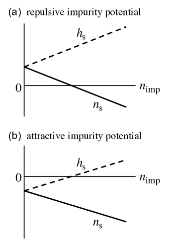
Figure 1: Normalized spin Nernst coefficient, $n_{\rm s}$ in Eq.(55) and the normalized spin Hall coefficient, $h_{\rm s}$ in Eq.(59) , as a function of the impurity density, $n_{\rm imp}$, for (a) a repulsive impurity potential and for (b) an attractive impurity potential.

III.2 Comparison with the spin Hall coefficient

We compare the dependence of the spin Nernst coefficient on the impurity density with that of the spin Hall coefficient derived in Ref.Hankiewicz and Vignale, 2006. We apply the number current along the $x$ axis, while we keep the spin current vanishing. We also set the condition that the current along the $y$ axis is vanishing for both the number and the spin, and that the electron temperature is uniform. The condition of $j_{y}^{\rm s}=0$ with $\nabla_{x}T_{\rm e}=0$ in Eq.(50) gives immediately

$$\nabla_{y}\mu^{\rm s}_{\rm ec}=H_{\rm s}\nabla_{x}\mu^{\rm n}_{\rm ec},$$ (57)

with the spin Hall coefficient $H_{\rm s}$ given by

$$H_{\rm s}=-\frac{L^{\rm sn}_{yx}}{L^{\rm ss}_{yy}}=2\ \frac{L_{xy}^{11\uparrow}}{L_{xx}^{11\uparrow}}.$$ (58)

When the electron gas is degenerate, we obtain

$$H_{\rm s}=2h_{\rm s},\ \ h_{\rm s}=-\frac{\tau_{\rm n}(\mu)}{\tau_{\rm ss}(\mu)}+\frac{2m\alpha}{\tau_{\rm n}(\mu)},$$ (59)

which reproduces the dependence of the spin Hall conductivity on $\tau_{\rm n}$ and $\tau_{\rm ss}$ derived in 2DES by Hankiewicz and Vignale.Hankiewicz and Vignale (2006) Comparing this formula of $h_{\rm s}$ with that of $n_{\rm s}$ in Eq.(55), the difference appears only at the sign of the second term from the side jump: the slope of $h_{\rm s}$ as a function of $n_{\rm imp}$ is positive, while that of $n_{\rm s}$ is negative. Therefore the change in sign of $h_{\rm s}$ with $n_{\rm imp}$ appears for the attractive impurity potential as shown in Fig.1.

The sample in the experiment by Sih et al.,Sih et al. (2005) in which Si donors are doped in the quantum well, corresponds to the attractive impurity potential in Fig.1(b). According to the calculation for this sample by Hankiewicz and Vignale,Hankiewicz and Vignale (2006) the contribution to the spin Hall conductivity from the side jump is comparable in size to that from the skew scattering. Therefore we expect that the sign change of the spin Hall coefficient should be observed if the density of Si impurities in the well is changed around the value of the Si density used in the experiment.

A Be impurity in GaAs is known to act as an acceptor. Therefore doping Be in a quantum well introduces the repulsive impurity potential for the 2DES.Haug et al. (1987) In this case it is expected, according to the calculated result in Fig.1(a), that the spin Nernst coefficient changes its sign as a function of the density of Be impurities.

IV Conclusions

We have studied theoretically the spin Nernst effect due to the spin-orbit interaction in the extrinsic origin in two-dimensional electron systems (2DES) in the $xy$ plane by employing the Boltzmann equation. We consider a 2DES confined within a symmetric quantum well with delta doping at the center of the well. We have shown in such a 2DES that the spin-orbit interaction, including that induced by the impurity potential, is diagonal in the $z$ component of spin because of the symmetry of the system.

In this model of 2DES we have investigated the dependence of the spin Nernst coefficient on the sign of the impurity potential and on the impurity density, and compared the result with that of the spin Hall coefficient. We have found that the spin Nernst coefficient changes its sign as a function of the impurity density in the case of the repulsive impurity potential, while no sign change occurs for the attractive impurity potential. On the other hand, the spin Hall coefficient changes its sign in the case of the attractive impurity potential, as shown already by Hankiewicz and Vignale.Hankiewicz and Vignale (2006) The sign change of each coefficient occurs due to the cancellation between the skew-scattering contribution and the side-jump contribution.

References

• Sinova et al. (2006) J. Sinova, S. Murakami, S. Q. Shen,  and M. S. Choi, Solid State Commun. 138, 214 (2006).
• Dyakonov and Khaetskii (2008) M. I. Dyakonov and A. V. Khaetskii, in Spin Physics in Semiconductors, edited by M. I. Dyakonov (Springer Berlin Heidelberg, 2008) pp. 211–243.
• Vignale (2010) G. Vignale, J. Supercond. Nov. Magn. 23, 3 (2010).
• Žutić et al. (2004) I. Žutić, J. Fabian,  and S. D. Sarma, Rev. Mod. Phys. 76, 323 (2004).
• Kato et al. (2004) Y. K. Kato, R. C. Myers, A. C. Gossard,  and D. D. Awschalom, Science 306, 1910 (2004).
• Wunderlich et al. (2005) J. Wunderlich, B. Kaestner, J. Sinova,  and T. Jungwirth, Phys. Rev. Lett. 94, 47204 (2005).
• Sih et al. (2005) V. Sih, R. C. Myers, Y. K. Kato, W. H. Lau, A. C. Gossard,  and D. D. Awschalom, Nat. Phys. 1, 31 (2005).
• Murakami et al. (2003) S. Murakami, N. Nagaosa,  and S.-C. Zhang, Science 301, 1348 (2003).
• Sinova et al. (2004) J. Sinova, D. Culcer, Q. Niu, N. A. Sinitsyn, T. Jungwirth,  and A. H. MacDonald, Phys. Rev. Lett. 92, 126603 (2004).
• Dyakonov and Perel (1971a) M. I. Dyakonov and V. I. Perel, Sov. Phys. JETP 13, 467 (1971a).
• Dyakonov and Perel (1971b) M. I. Dyakonov and V. I. Perel, Phys. Lett. A 35, 459 (1971b).
• Hirsch (1999) J. E. Hirsch, Phys. Rev. Lett. 83, 1834 (1999).
• Zhang (2000) S. Zhang, Phys. Rev. Lett. 85, 393 (2000).
• Engel et al. (2005) H.-A. Engel, B. I. Halperin,  and E. I. Rashba, Phys. Rev. Lett. 95, 166605 (2005).