Generalized rotating-wave approximation to biased qubit-oscillator systems

Abstract

The generalized rotating-wave approximation with counter-rotating interactions has been applied to a biased qubit-oscillator system. Analytical expressions are explicitly given for all eigenvalues and eigenstates. For a flux qubit coupled to superconducting oscillators, spectra calculated by our approach are in excellent agreement with experiment. Calculated energy levels for a variety of biases also agree well with those obtained via exact diagonalization for a wide range of coupling strengths. Dynamics of the qubit has also been examined, and results lend further support to the validity of the analytical approximation employed here. Our approach can be readily implemented and applied to superconducting qubit-oscillator experiments conducted currently and in the near future with a biased qubit and for all accessible coupling strengths.

I Introduction

The combination of a two-level system (or a qubit) and a harmonic oscillator has found myriad interesting applications in quantum systems ranging from two-level atoms coupled to optical or microwave cavities Scully ; Buluta to superconducting qubits coupled to superconducting resonators schuster ; Wallraff ; chio ; you ; nation . In early work on cavity quantum electrodynamics (QED), the qubit-oscillator coupling strength $g$ achieved was much smaller than the cavity transition frequency $\omega$, i.e., $g/\omega\sim 0.001$. Experiments can therefore be well described by the Jaynes-Cumming model with the rotating-wave approximation (RWA) jaynes .

In recent circuit QED setups, where artificial superconducting two-level atoms are coupled to on-chip cavities, the exploration of quantum physics has greatly evolved in the ultrastrong coupling regime, where the atom-cavity coupling strength is comparable to the cavity transition frequency, $g/\omega\sim 0.1$ Wallraff ; chio ; Niemczyk ; pfd ; fedorov . It is evident for the breakdown of the RWA and the counter-rotating terms are expected to take effect. There have been numerous theoretical studies on the qubit-oscillator system finding new phenomena in the ulrastrong coupling regime  Ashhab ; grifoni ; irish ; feranchuk ; amniat and deep strong coupling regime with $g/\omega>1$ casanova ; zhang . However, many theories are derived for an unbiased qubit, or in the terminology of cavity and circuit QED, for a qubit operated at the degeneracy point or the sweet spot. While the unbiased qubit is often encountered for real atoms in cavity QED, it is quite straightforward to vary the static bias of superconducting qubits by adjusting an external control parameter such as the gate voltage applied the magnetic flux acting on a Josephson junction Niemczyk ; pfd ; fedorov . Therefore, it is necessary to develop theories which adequately treat the biased qubit-oscillator system. Taking the qubit’s bias into account, Grifoni et al. grifoni formulated the Van Vleck perturbation (VVP) theory beyond the RWA to treat analytically a two-level system coupled to a harmonic oscillator. Unfortunately, it gives unphysical energy-level crossings in the weak coupling regime for positive detuning. An adiabatic approximation was proposed by Nori et al. Ashhab for a biased system in various parameter regimes. Existing approaches to describe the behavior of the biased system are often suited for a particular circumstance, despite that many analytical methods have been proposed. An efficient, accurate treatment of the biased qubit-oscillator system in all parameter regimes remains elusive.

In this work a generalized rotating-wave approximation (GRWA) is proposed for the biased qubit-oscillator system in the ulstrastrong coupling regime, extending the pioneering work of Irish on unbiased system irish , an approach that we shall call the biased generalized rotating-wave approximation (BGRWA). Our analytical approach takes into account the effect of qubit-oscillator counter-rotating terms, while the renormalized Hamiltonian including energy-conserving terms retains the mathematical simplicity of the usual RWA. This easily-implemented approach gives simple analytical expressions for eigenvalues and eigenvectors for the ground and low-lying excited states, and is applicable to a wide range of the coupling parameters. In the limit of zero bias, we recover the early results of Irish irish which were obtained for an unbiased qubit using GRWA. By parameter-fitting the circuit QED experiment, an analytical experssion is obtained for the energy spectrum in the ulstrastrong coupling regime. Validity of our approach is discussed by comparing with the VVP method as well as numerical exact diagonalization. Furthermore, we also study the qubit dynamics in the ultrastrong coupling regime to confirm the effectiveness of the BGRWA.

The paper is outlined as follows. In Sec. II, we derive expressions for the eigenenergies and eigenstates of a biased qubit-oscillator system using BGRWA. Analytical expressions for the spectrum is also given by fitting the circuit QED experiment. In Sec. III, we discuss the qubit dynamics in the finite bias case. Finally, a brief summary is given in Sec. IV.

II analytical solution

The Hamiltonian of the qubit can be written as $H_{q}=-(\varepsilon\sigma_{x}+\Delta\sigma_{z})/2$, where $\sigma_{x}$ and $\sigma_{z}$ are Pauli matrices; $\Delta$ is the tunneling parameter between the upper level $|+z\rangle$ and the lower level $|-z\rangle$ in the basis of $\sigma_{z}$; $\varepsilon$ is the magnetic energy bias related to the circulating current in the qubit loop and the applied magnetic flux pfd ; fedorov . In the weak coupling regime, where the interaction strength $g$ exceeds the cavity and qubit loss rates, the RWA can be applied and the system can be described by the Jaynes-Cummings-type Hamiltonian for zero bias as

$$H=\frac{\Delta}{2}\sigma_{z}+\omega a^{\dagger}a+g(a^{\dagger}\sigma_{-}+a\sigma_{+}),$$ (1)

where $a^{\dagger}$ and $a$ are the creation and annihilation operators for the oscillator, and we have set $\left(\hbar\right)$ to unity. The Jaynes-Cummings-type Hamiltonian (1) can be solved analytically in a closed form in the basis $|n\rangle|+z\rangle$ and $|n+1\rangle|-z\rangle$, where the qubit states $|\pm z\rangle$ are eigenstates of $\sigma_{z}$, and the oscillator states $|n\rangle$ ($n=0,1,2,...$) are Fock states. The ground state obtained is $|\psi_{g}\rangle=|0\rangle|-z\rangle$ for weak coupling. However, current experimental advances draw our attention to the ultrastrong coupling regime, where $g$ approaches to the qubit or oscillator frequencies, and the RWA no longer holds Niemczyk ; pfd ; fedorov . Thus, the qubit-oscillator counter-rotating interaction $a^{\dagger}\sigma_{+}+a\sigma_{-}$ needs to be taken into account.

Under a rotation around the $y$ axis with the angle $\pi/2$, the Hamiltonian of the qubit-oscillator system including the counter-rotating terms reads

$$H=-\frac{\Delta}{2}\sigma_{x}-\frac{\varepsilon}{2}\sigma_{z}+\omega a^{\dagger}a+g(a^{\dagger}+a)\sigma_{z}.$$ (2)

Making use of a unitary transformation $U=\exp\left[-\frac{g}{\omega}\sigma_{z}\left(a-a^{\dagger}\right)\right],$ we can obtain a transformed Hamiltonian $H^{{}^{\prime}}=U^{\dagger}HU=H_{0}+H_{1}$, consisting of

$$H_{0} = \omega a^{\dagger}a-g^{2}/\omega-\frac{\varepsilon}{2}\sigma_{z},$$ (3)

$$H_{1} = -\frac{\Delta}{2}\{\sigma_{x}\cosh[\frac{2g}{\omega}\left(a^{\dagger}-a\right)]+i\sigma_{y}\sinh[\frac{2g}{\omega}\left(a^{\dagger}-a\right)]\}.$$

Recently, much theoretical attention has been devoted to the qubit-oscillator system using a variety of transformations grifoni ; irish ; yu ; zheng ; talab . In particular, Irish has presented a generalized version of the RWA by performing a simple basis change prior to eliminating the counter-rotating terms irish . This gives rise to a significantly more accurate expression for the energy levels of the system for all values of the coupling strength. We now extend the generalized RWA by Irish to the biased qubit-oscillator system. The simplicity of the approximation is based on its close connection to the standard RWA. Consequently, the terms retained in $H_{1}$ correspond to the energy-conserving one-excitation terms, just as in the standard RWA. When $\cosh\left[\frac{2g}{\omega}\left(a^{\dagger}-a\right)\right]$ is expanded as $1+\frac{1}{2!}[\frac{2g}{\omega}\left(a^{\dagger}-a\right)]^{2}+\frac{1}{4!}[\frac{2g}{\omega}\left(a^{\dagger}-a\right)]^{4}+...,$ it is performed by keeping the terms containing the number operator $a^{\dagger}a=n$ with the coefficient $G_{0}\left(n\right)$

$$G_{0}(n) =\langle n|\cosh[\frac{2g}{\omega}(a^{\dagger}-a)]|n\rangle$$ (5)

$$=\exp(-2g^{2}/\omega^{2})L_{n}(4g^{2}/\omega^{2}),$$

where $L_{n}$ are the Laguerre polynomials. Higher-order excitation terms such as $a^{\dagger 2}$, $a^{2}$,…, which are accounted for multi-photon process, are neglected within this approximation. Similarly, by expanding $\sinh[\frac{2g}{\omega}\left(a^{\dagger}-a\right)]=\frac{2g}{\omega}\left(a^{\dagger}-a\right)+\frac{1}{3!}[\frac{2g}{\omega}\left(a^{\dagger}-a\right)]^{3}+\frac{1}{5!}[\frac{2g}{\omega}\left(a^{\dagger}-a\right)]^{5}+...,$ the one-excitation terms are kept as $F_{1}\left(n\right)a^{\dagger}-aF_{1}\left(n\right)$ with the coefficient $F_{1}\left(n\right)$ to be determined. Since the terms $aF_{1}\left(n\right)$ and $F_{1}\left(n\right)a^{\dagger}$ involve creating and eliminating a single photon of the oscillator, it can be evaluated as

$$F_{1}\left(n\right) =\frac{1}{\sqrt{n+1}}\left\langle n+1\right|\sinh\left[\frac{2g}{\omega}\left(a^{\dagger}-a\right)\right]\left|n\right\rangle$$ (6)

$$=\frac{2g}{\omega(n+1)}e^{-2g^{2}/\omega^{2}}L_{n}^{1}(4g^{2}/\omega^{2}).$$

Since the higher-order terms of $H_{1}$ are discarded, we can construct an effective Hamiltonian $H^{{}^{\prime}}=H_{0}^{{}^{\prime}}+H_{1}^{{}^{\prime}}$ with

$$H_{0}^{{}^{\prime}} = \omega a^{\dagger}a-g^{2}/\omega-\frac{\Delta\eta}{2}\sigma_{x}-\frac{\varepsilon}{2}\sigma_{z},$$

$$H_{1}^{{}^{\prime}} = -\frac{\Delta}{2}[G_{0}(n)-\eta]\sigma_{x}-i\frac{\Delta}{2}\sigma_{y}F_{1}(n)(a^{\dagger}-a),$$

where the parameter $\eta$ is defined as $\eta=G_{0}(0)$.

As the qubit and oscillator are decoupled in $H_{0}^{{}^{\prime}}$ and its qubit part can be diagonalized by a second unitary transformation $S=\left(\begin{array}[]{ll}u&v\\ v&-u\end{array}\right)$ with $u=\frac{1}{\sqrt{2}}\sqrt{1-\frac{\varepsilon}{y}}$, $v=\frac{1}{\sqrt{2}}\sqrt{1+\frac{\varepsilon}{y}}$, and $y=\sqrt{\varepsilon^{2}+\Delta^{2}\eta^{2}}$. The diagonalized $H_{0}^{{}^{\prime}}$ takes the form

$$\tilde{H_{0}} = S^{+}H_{0}^{{}^{\prime}}S=\omega a^{\dagger}a-g^{2}/\omega+\frac{1}{2}\sqrt{\varepsilon^{2}+\Delta^{2}\eta^{2}}\sigma_{z},$$

where the tunneling parameter is renormalized by $\sqrt{\varepsilon^{2}+\Delta^{2}\eta^{2}}/2$. And the $H_{1}^{{}^{\prime}}$ is transformed into

$$\tilde{H_{1}} = S^{+}H_{1}^{{}^{\prime}}S$$ (9)

$$= \frac{\Delta^{2}\eta[G_{0}(n)-\eta]}{2\sqrt{\varepsilon^{2}+\Delta^{2}\eta^{2}}}\sigma_{z}-\frac{\Delta}{2}F_{1}(n)(\sigma_{+}-\sigma_{-})(a^{\dagger}-a)$$

$$- \frac{\Delta\varepsilon[G_{0}(n)-\eta]}{2\sqrt{\varepsilon^{2}+\Delta^{2}\eta^{2}}}\sigma_{x}.$$

In order to cast the second term in Eq. (9), representing the qubit-socillator interactions in $\tilde{H_{1}}$, into the same form as the ordinary RWA term in Eq. (1), the Hamiltonian under BGRWA can be approximated by the form

$$H_{\rm BGRWA}=\omega a^{\dagger}a-g^{2}/\omega+\varepsilon(n)\sigma_{z}+R_{r}(a^{\dagger}\sigma_{-}+a\sigma_{+}),$$

where the tunneling parameter $\varepsilon(n)$ is renormalized to

$$\varepsilon(n)=\frac{\varepsilon^{2}+\Delta^{2}\eta G_{0}(n)}{2\sqrt{\varepsilon^{2}+\Delta^{2}\eta^{2}}},$$ (11)

and the effective coupling strength is $R_{r}=\Delta F(n)/2$, which depends on the parameters $\Delta$ and $g$. The Hamiltonian after the transformation retaining the mathematical structure of the ordinary RWA contains the counter-rotating terms, which play an important role in the ultrastrong coupling regime.

Our aim is to extend the GRWA derivation to qubit-oscillator systems with a finite bias. Similar to the GRWA employed by Irish irish , only zero- and one-excitation terms are kept in the transformed Hamiltonian in terms of $G_{0}(n)$ and $F_{1}(n)$. Unlike the GRWA for zero bias, we take into account the static bias of the qubit while adjusting the renormalized tunneling parameter $\varepsilon(n)$, a term also present in the transformation of the biased spin-boson model by Gan and Zheng zheng . The effective Hamiltonian (II) with the counter-rotating interactions contains the energy-conserving term $R_{r}(a^{+}\sigma_{-}+a\sigma_{+})$, which is identical in form to the corresponding term in the usual RWA Hamiltonian (1). A simplified expression for a biased qubit system, our approximation is expected to extend the range of validity to the ulstrastrong coupling regime for qubit-oscillator systems with a finite bias.

One can easily diagonalize the Hamiltonian (II) in the basis of $|+z,n\rangle$ and $|-z,n+1\rangle$

$$H_{\rm BGRWA}=\left(\begin{array}[]{ll}\omega n-g^{2}/\omega+\varepsilon(n)&R_{r}(n)\sqrt{n+1}\\ R_{r}(n)\sqrt{n+1}&\omega(n+1)-g^{2}/\omega-\varepsilon(n)\end{array}\right).$$ (12)

It is straightforward to obtain the eigenvalues

$$E_{n}^{\pm,{\rm BGRWA}} = \omega(n+\frac{1}{2})-g^{2}/\omega+\frac{\Delta^{2}\eta}{4\sqrt{\varepsilon^{2}+\Delta^{2}\eta^{2}}}e^{-2g^{2}/\omega^{2}}[L_{n}(4g^{2}/\omega^{2})-L_{n+1}(4g^{2}/\omega^{2})]$$

$$\pm\{[\frac{\omega}{2}-\frac{2\varepsilon^{2}+\Delta^{2}\eta e^{-2g^{2}/\omega^{2}}[L_{n}(4g^{2}/\omega^{2})+L_{n+1}(4g^{2}/\omega^{2})]}{4\sqrt{\varepsilon^{2}+\Delta^{2}\eta^{2}}}]^{2}+\frac{g^{2}\Delta^{2}e^{-4g^{2}/\omega^{2}}}{\omega^{2}(n+1)}[L_{n}^{1}(4g^{2}/\omega^{2})]^{2}\}^{1/2},$$

and the corresponding eigenfunctions

$$|\varphi_{n}^{+}\rangle = \cos\frac{\theta}{2}|n\rangle|+z\rangle+\sin\frac{\theta}{2}|n+1\rangle|-z\rangle,$$ (14)

$$|\varphi_{n}^{-}\rangle = \sin\frac{\theta}{2}|n\rangle|+z\rangle-\cos\frac{\theta}{2}|n+1\rangle|-z\rangle,$$ (15)

where

$$\theta = \arccos\frac{\delta}{\sqrt{\delta^{2}+4R_{r}^{2}(n+1)}}$$

$$\delta = \frac{2\varepsilon^{2}+\Delta^{2}\eta[L_{n}(4g^{2}/\omega^{2})+L_{n+1}(4g^{2}/\omega^{2})]}{2\sqrt{\varepsilon^{2}+\Delta^{2}\eta^{2}}}-\omega$$

In the case of $\varepsilon=0$, the eigenvalues in Eq. (II) are reduced to the GRWA form irish . The energy for the ground-state $|-z,0\rangle$ is

$$E_{g}^{\rm BGRWA}=-\frac{1}{2}\sqrt{\varepsilon^{2}+\Delta^{2}\eta^{2}}-g^{2}/\omega.$$ (16)

Thanks to the recent advances in experiment, new spectral observations on qubit-oscillator systems are made available in the ultrastrong coupling regime pfd , which were fitted by exact diagonalization using the Fock basis pfd and the coherent-state basis lei . In the setup of a flux qubit coupled to an superconducting oscillator, the bias parameter $\varepsilon=2I_{p}(\Phi-\Phi_{0}/2)$ with $I_{p}$ the persistent current in the qubit loop, $\Phi$ an externally applied magnetic flux, and $\Phi_{0}=\hbar/2e$ the flux quantum. Fig. 1 shows the spectrum of the system using Eqs. (II) and (16), with fitted parameters of the experimental results $g/2\pi=0.82~{}\rm{GHz}$, $\omega/2\pi=8.13~{}\rm{GHz}$, $\Delta=4.25~{}\rm{GHz}$ and $I_{p}=510~{}nA$. No substantial difference is found between our results and experiment ones as shown in Fig. 3 of Ref. pfd . This demonstrates the great potential of our BGRWA approach to be applied in future experiment as increasingly larger coupling strengths become accessible.

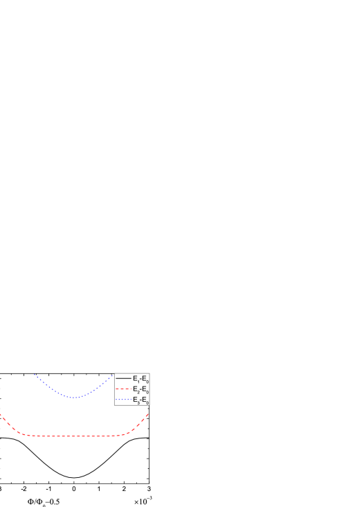
Figure 1: Spectrum of the qubit coupled to an oscillator obtained from Eqs. (II) and (16) using the experiment parameters in Ref pfd .

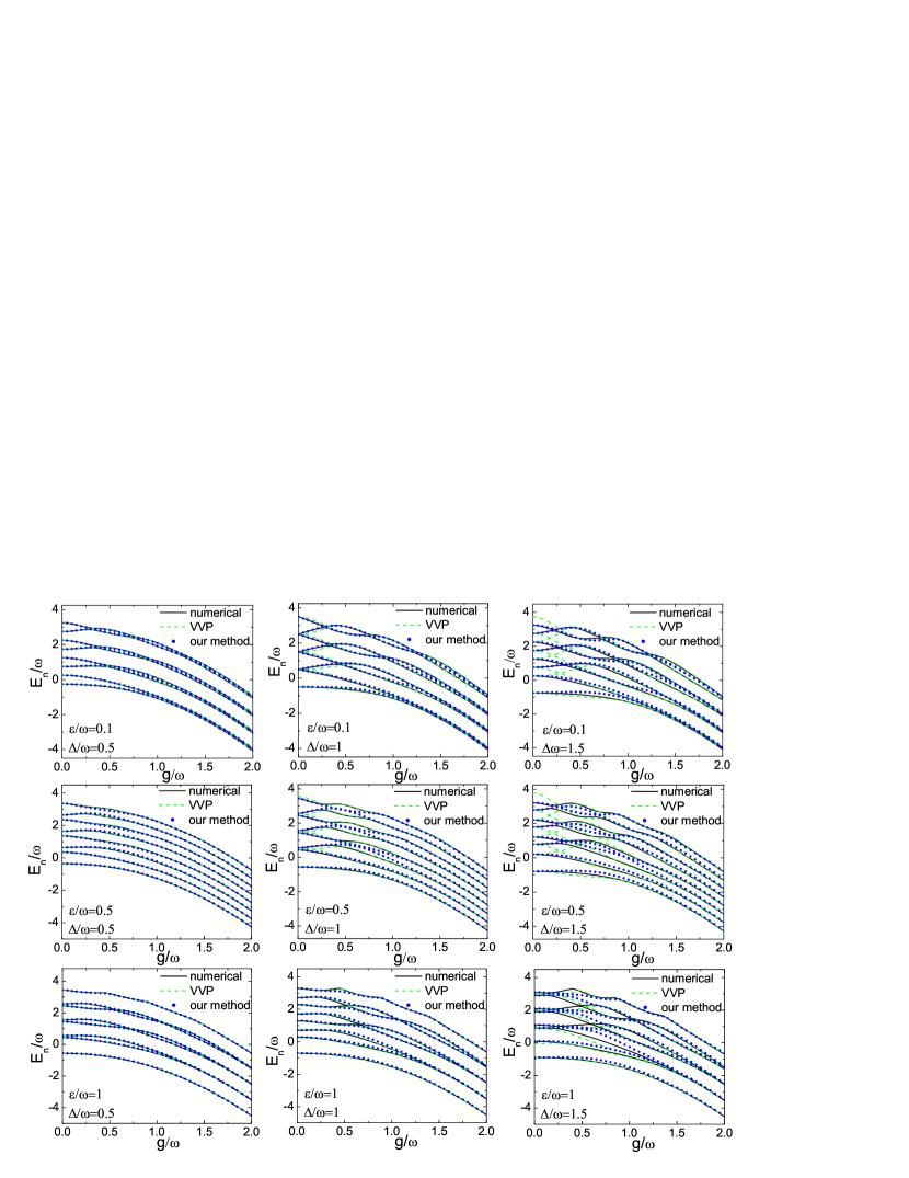
Figure 2: Energy levels $E_{n}$ as a function of coupling strength $g$ for different bias $\varepsilon=0.1$, $0.5$ and $1$ (from top to bottom) with the tunneling parameter $\Delta=0.5$, $1$ and $1.5$. We compare the eigenvalues in Eq. (II) (solid dot) with those obtained by the numerical exact diagonalization method (solid line) and VVP eigenvalues in Eq. (II)(dashed line). We set $\omega=1$.

To the best of our knowledge, Eqs. (II)-(16), obtained using our BGRWA approach, is the simplest among all existing analytical expressions. Provided that its validity is verified in general, the BGRWA approach is a potentially effective tool in the study of the superconducting qubit-oscillators where the biased parameter can be adjusted externally. To this end, we present here a detailed discussion on the energy spectrum of the biased qubit-oscillator system. First, we consider eigenvalues obtained by the VVP method, which can be written as  grifoni

$$E_{m}^{\pm} = (m+\frac{l}{2})\omega-\frac{g^{2}}{\omega}+\frac{1}{2}\sum_{k=0,k\neq m\pm l}(\frac{D_{mk}^{2}}{\varepsilon+(m-k)\omega}-\frac{D_{nk}^{2}}{\varepsilon+(k-n)\omega})$$

$$\pm \frac{1}{2}\sqrt{[\varepsilon-l\omega+\Delta^{2}\sum_{k=0,k\neq m\pm l}(\frac{D_{mk}^{2}}{\varepsilon+(m-k)\omega}+\frac{D_{nk}^{2}}{\varepsilon+(k-n)\omega})]^{2}+4D_{mn}^{2}},$$

$$(n = m+l,l\geq 0)$$ (17)

where $D_{mn}=\frac{\Delta}{2}(-1)^{m}(2g)^{n-m}e^{-2g^{2}}\sqrt{\frac{m!}{n!}}L_{m}^{n-m}(4g^{2}/\omega^{2})$. The $m$th eigenvalues $E_{m}^{\pm}$ is a mixture of the oscillator levels $m$ and $l$. Note the ambiguity of the value of $l$, which is selected to give better results. The VVP method works well for large values of the bias $\varepsilon$ and strong qubit-oscillator coupling. In comparison, our analytical expression of eigenvalues as given in Eq. (II) can be more easily implemented. Below we will give a detailed comparison for various values of the coupling strength $g$ and detuning parameter $\Delta/\omega$.

Fig. 2 displays the first eight energy levels as a function of the coupling strength $g$ for various values of the bias $\varepsilon$ and the tunneling parameter $\Delta$. Here we set $\omega=1$. For negative detuning $\Delta=0.5$, our analytical approach and the VVP method are in good agreement with the numerical exact-diagonalization results from the weak coupling regime to the strong coupling regime for $\varepsilon=0.1$, $0.5$ and $1$, as shown in the left column of Fig. 2. At the resonance $\Delta=1$ (middle column), our analytical solutions agree well with the numerical results for $g<0.5$, a coupling strength range that is either currently accessible ($g<0.12$) Niemczyk or will be made accessible in the near future. In this interesting coupling regime of $g<0.5$, the VVP results deviate considerably from the numerical ones. In the intermediate coupling regime ($0.5<g<1$), there is a noticeable difference between results from our method and those from the exact diagonalization due to the dominant influence of the higher-order terms neglected in the transformed hamiltonian in Eq. (II) accompanied by more photon excitations. In the case of positive detuning $\Delta=1.5$, substantial improvements of our approach over the VVP method can be seen in the weak coupling regime, as shown in the right column of Fig. 2. Especially, for $\varepsilon=0.1$ and $0.5$, the VVP results in the weak coupling regime are qualitatively incorrect with an unphysical crossing. In comparison, our BGRWA results remain in agreement with the numerically exact ones one. Therefore, the BGRWA approach, which takes into account the effect of counter-rotating terms, provides an efficient, yet accurate analytical expressions to the energy spectrum of the biased qubit-oscillator system.

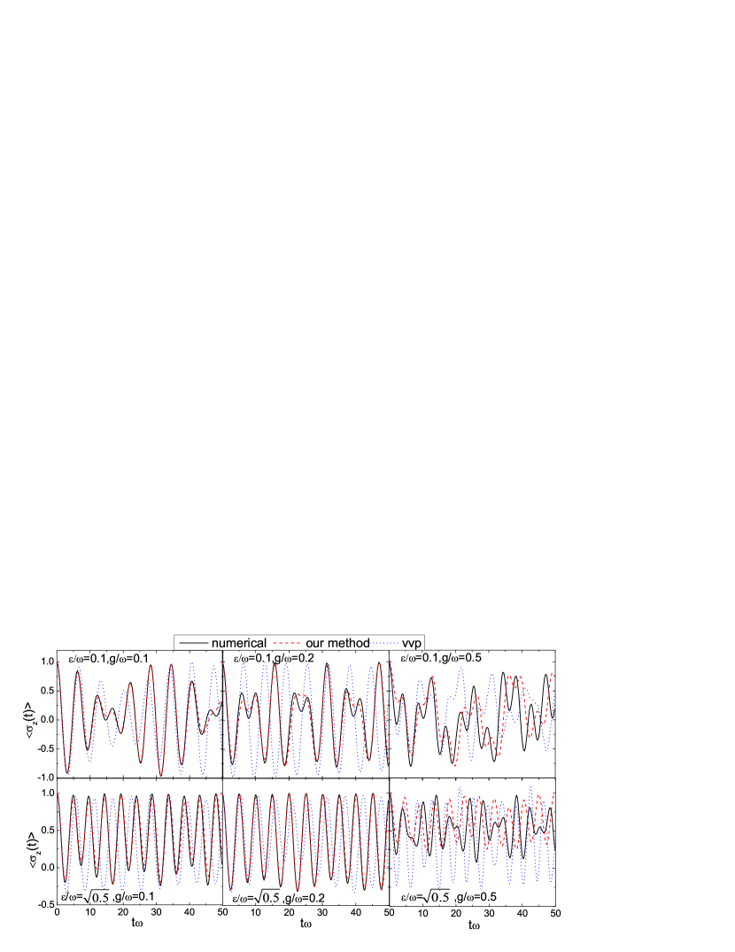
Figure 3: Time evolution of $\sigma_{z}(t)$ for $\varepsilon=0.1$ (upper panel) and $\sqrt{0.5}$ (low panel) for different coupling strength $g=0.1,0.2,0.5$ on resonance. The dashed line is our BGRWA calculation. The solid and the dotted line are the numerically exact result and the VVP one, respectively. The evolution starts with a vacuum oscillator state $|0\rangle$ and an excited spin $|e\rangle$.

III dynamics of the qubit

In the original Hamiltonian (2) with counter-rotating terms, the excited wave functions without RWA can be obtained using a unitary transformation $|\Psi_{n}^{\pm}\rangle=U^{+}S^{+}|\varphi_{n}^{\pm}\rangle$:

$$|\Psi_{n}^{+}\rangle^{\rm BGRWA} = (u\cos\frac{\theta}{2}|n\rangle_{\frac{g}{\omega}}+v\sin\frac{\theta}{2}|n+1\rangle_{\frac{g}{\omega}})|+x\rangle$$

$$+ (v\cos\frac{\theta}{2}|n\rangle_{\frac{-g}{\omega}}-u\sin\frac{\theta}{2}|n+1\rangle_{\frac{-g}{\omega}})|-x\rangle,$$

$$|\Psi_{n}^{-}\rangle^{\rm BGRWA} = (u\sin\frac{\theta}{2}|n\rangle_{\frac{g}{\omega}}-v\cos\frac{\theta}{2}|n+1\rangle_{\frac{g}{\omega}})|+x\rangle$$

$$+ (v\sin\frac{\theta}{2}|n\rangle_{\frac{-g}{\omega}}-u\cos\frac{\theta}{2}|n+1\rangle_{\frac{-g}{\omega}})|-x\rangle,$$

where the qubit states $|\pm x\rangle$ are eigenstates of $\sigma_{x}$, and the oscillator states $|n\rangle_{{}_{\pm g/\omega}}=e^{\mp g/\omega(a-a^{\dagger})}|n\rangle$ are displaced Fock states, or the so-called coherent states. The ground-state wave function is obtained by

$$|\Psi_{g}\rangle^{\rm BGRWA}=v|e\rangle e^{-g/\omega(a-a^{\dagger})}|0\rangle-u|g\rangle e^{g/\omega(a-a^{\dagger})}|0\rangle.$$

Next we examine the time evolution of $\sigma_{z}(t)$ to further demontrate the validity of our analytical approach. The initial state is assumed as $|\varphi(0)\rangle=|\uparrow\rangle|0\rangle$. Using the eigenvectors $\{|\Psi_{n}\rangle^{\rm BGRWA}\}$ and eigenevalues $\{E_{n}^{\rm BGRWA}\}$, the dynamical wave function of the Hamiltonian (2) without RWA can be expressed as

$$|\varphi(t)\rangle =e^{-iHt}|\varphi(0)\rangle$$

$$=\sum_{n}e^{-itE_{n}^{\rm BGRWA}}|\Psi_{n}\rangle^{\rm BGRWA}\langle\Psi_{n}|\varphi(0)\rangle.$$

Using our approach without RWA for the biased system, $\langle\sigma_{z}(t)\rangle=\langle\varphi(t)|\sigma_{z}|\varphi(t)\rangle$ has been calculated, and results are plotted in Fig. 3 for $\varepsilon=0.1$ (upper panel) and $\sqrt{0.5}$ (lower panel) for coupling strengths $g=0.1,0.2,0.5$. For comparison, results from exact diagonalization and those of VVP are also shown. It is found that the time-dependent analytical results agree well with the numerical ones, with substantial improvements over those obtained by VVP. It follows that the contribution of the counter-rotating interaction is well taken in account in the BGRWA analytical solution. Thus, our BGRWA approach is valid in a wide range of coupling strengths for dynamic simulation of the wave functions.

IV conclusion

Analytical expressions without the RWA have been derived for the energy spectrum of the qubit-oscillator system with a finite bias. Our approach takes into account the counter-rotating interactions while retaining mathematical simplicity of the ordinary RWA. Eigenvectors and eigenvalues obtained analytically recover the results of GRWA at zero bias, and the BGRWA approximation is valid even in the ultrastrong coupling regime. Our analytical spectrum expressions are shown in good agreement with experiment, and in comparison with energy levels calculated using the VVP method and exact diagonalization, exhibit a wide range of validity for coupling strengths $g<0.5$. Energy levels of the ground and lower-lying excited states obtained in this work show substantial improvements over the VVP results. In particular, our analytical expressions for the energy levels fit well with exact diagonalization results in the positive detuning regime, where the VVP method is invalid. Moreover, time evolution of $\sigma_{z}(t)$ obtained using BGRWA is in quantitative agreement with the exact diagonalization result for weak and ultra-strong couplings. The analytical approach presented here can be easily implemented to simulate superconducting qubit-oscillator systems for coupling strengths up to $g=0.5$. Finally, our approach can be employed to tackle problems of higher complicity such as a biased spin-boson model.

- (1) M. O. Scully and M. S. Zubairy, Quantum Optics, Cambridge University Press, Cambridge, 1997; M. Orszag, Quantum Optics: Including Noise Reduction,Trapped Ions, Quantum Trajectories, and Decoherence, Science publish, (2007); D. F. Walls and G. J. Milburn, Quantum Optics (Springer Verlag, Berlin, 1994).
- (2) I. Buluta et al., Science 326, 108 (2009); Reports on Progress in Physics 74,104401 (2011).
- (3) D. I. Schuster et al., Nature (London) 445, 515(2007)
- (4) A. Wallraff et al., Nature (London)431, 162(2004).
- (5) I. Chiorescu, P. Bertet, K. Semba, Y. Nakamura, C. J. P. M. Harmans, and J. E. Mooij, Nature (London) 431, 159(2004).
- (6) J.Q. You et al., Phys. Today 58, 42 (2009); Nature 474, 589 (2011); Phys. Rev. B. 68, 024510 (2003); Phys. Rev. B. 68, 064509 (2003).
- (7) P.D. Nation et al., Rev. Mod. Phys. 84, 1 (2012).
- (8) E.T. Jaynes, and F.W. Cummings, Proc. IEEE. 51, 89(1963).
- (9) T. Niemczyk et al., Nature Physics 6, 772(2010).
- (10) P. Forn-Díaz et al., Phys. Rev. Lett. 105, 237001 (2010).
- (11) A. Fedorov et al., Phys. Rev. Lett. 105, 060503 (2010).
- (12) S. Ashhab and F. Nori, Phys. Rev. A 81, 042311 (2010).
- (13) J. Hausinger and M. Grifoni, Phys. Rev. A. 82, 062320 (2010).
- (14) E.K. Irish, Phys. Rev. Lett. 99, 173601(2007).
- (15) I D Feranchuk, L I Komarov, and A P Ulyanenkov, J. Phys. A: Math. Gen. 29, 4035 (1996).
- (16) M Amniat-Talab, S Guerin, and H R Jauslin, J. Math. Phys. 46, 042311 (2005).
- (17) J. Casanova, G. Romero, I. Lizuain, J. J. Garcia-Ripoll, and E. Solano, Phys. Rev. Lett. 105, 263603(2010).
- (18) Y. Y. Zhang, Q. H. Chen, and S. Y. Zhu, arXiv:1106.2191 (2011).
- (19) L. X. Yu, S. Q. Zhu, Q. F. Liang, G. Chen, and S. T. Jia, Phys. Rev. A 86, 015803 (2012).
- (20) C. J. Gan, and H. Zheng, Eur. Phys. J. D 59,473 (2010).
- (21) M. Amniat-Talab et al., J. Math. Phys. 46, 042311(2005).
- (22) Q.H. Chen, L. Li, T. Liu, and K.L. Wang, Chinese Phys. Lett. 29, 014208 (2012).