How quickly can we sample a uniform domino tiling of the $2L\times 2L$ square via Glauber dynamics?

Abstract.

The prototypical problem we study here is the following. Given a $2L\times 2L$ square, there are approximately $\exp(4KL^{2}/\pi)$ ways to tile it with dominos, i.e. with horizontal or vertical $2\times 1$ rectangles, where $K\approx 0.916$ is Catalan’s constant [7, 25]. A conceptually simple (even if computationally not the most efficient) way of sampling uniformly one among so many tilings is to introduce a Markov Chain algorithm (Glauber dynamics) where, with rate $1$, two adjacent horizontal dominos are flipped to vertical dominos, or vice-versa. The unique invariant measure is the uniform one and a classical question [28, 17, 16] is to estimate the time $T_{\rm mix}$ it takes to approach equilibrium (i.e. the running time of the algorithm). In [17, 20], fast mixing was proven: $T_{\rm mix}=O(L^{C})$ for some finite $C$. Here, we go much beyond and show that $cL^{2}\leq T_{\rm mix}\leq L^{2+o(1)}$. Our result applies to rather general domain shapes (not just the $2L\times 2L$ square), provided that the typical height function associated to the tiling is macroscopically planar in the large $L$ limit, under the uniform measure (this is the case for instance for the Temperley-type boundary conditions considered in [9]). Also, our method extends to some other types of tilings of the plane, for instance the tilings associated to dimer coverings of the hexagon or square-hexagon lattices.

2010 Mathematics Subject Classification: 60K35, 82C20, 52C20
Keywords: Domino tilings, Glauber dynamics, Perfect matchings, Mean curvature motion

1. Introduction

Uniform random perfect matchings (or dimer coverings) of a bipartite, infinite, planar periodic graph $G$ (e.g. ${\mathbb{Z}}^{2}$ or the hexagonal lattice $\mathcal{H}$) play a crucial role in statistical mechanics and combinatorics, and a vast literature exists on the subject (cf. for instance the classical papers [7, 25] and the much more recent [12]). On one hand, thanks to the bijection between perfect matchings and discrete height functions (see Section 2.1.1), they provide natural and exactly solvable models of random $(2+1)$-dimensional interfaces (which can be thought of as simplified models for the interface separating two coexisting thermodynamic phases [23]). On the other hand, thanks to their conformal invariance and Gaussian Free Field-like fluctuation properties in the scaling limit [9, 10, 12], they belong, like the Ising model at $T=T_{c}$, to the family of critical two-dimensional systems.

In contrast, the study of stochastic dynamics of perfect matchings is a much less developed topic. Typically, one takes a large but finite portion $G^{\prime}$ of the graph $G$ and defines a simple Glauber-type Markov chain such that each update locally modifies the matching within $G^{\prime}$. The unique equilibrium measure is the uniform measure over perfect matchings of $G^{\prime}$. From the point of view of theoretical computer science [17, 16, 28, 20], the interesting question is to understand how quickly, as a function of the size of $G^{\prime}$, the Markov chain approaches equilibrium (i.e. how quickly it samples reliably a uniformly chosen random perfect matching of $G^{\prime}$). From the point of view of statistical physics, thanks to the above mentioned bijection between perfect matchings and height functions, this Markov chain can be seen as a dynamics for a $(2+1)$-dimensional interface  and it is of interest to understand how the geometry of the interface evolves in time. For instance, when $G=\mathcal{H}$ the evolution of the height function exactly coincides with the zero-temperature heat-bath dynamics for an interface, separating “$-$” from “$+$” spins, of the three-dimensional nearest-neighbor Ising model [4].

Until recently, the best mathematical result on this dynamics issues was that, when $G={\mathbb{Z}}^{2}$ or $G=\mathcal{H}$, the total-variation mixing time $T_{\rm mix}$ of the Markov chain is at most polynomial in the size of $G^{\prime}$. See Section 1.1.1 for a short review. Results of this type are based on simple but effective coupling arguments that unfortunately have little chance of providing the sharp behavior of $T_{\rm mix}$. (A notable exception is the work [28], where sharp bounds on $T_{\rm mix}$ for $G=\mathcal{H}$ were given, but for a very particular, spatially non-local, dynamics).

In [5], instead, in the case where $G=\mathcal{H}$ it was proven that, under a certain condition on the shape of the finite region $G^{\prime}$ (“almost planar boundary condition” assumption, see below), $T_{\rm mix}$ behaves like $L^{2}$, up to logarithmic corrections, if $L$ is the diameter of $G^{\prime}$. As we briefly explain in Section 1.2, going beyond the case of the hexagonal lattice $\mathcal{H}$ is a mathematical challenge, since certain exact identities that hold there do not survive on more general graphs. In this work we prove that, when $G={\mathbb{Z}}^{2}$ (and in a few other cases, see below), again under the “planar boundary condition” assumption, $T_{\rm mix}=L^{2+o(1)}$. We present this result, still informally but with a bit more of detail, in the next section.

The major improvement with respect to [17, 28] is that both [5] and the present work use the intuition that the height function should evolve, on a diffusive time-space scale, according to a deterministic, anisotropic mean-curvature type evolution [23]. More precisely, call $h_{t}(X,Y)$ the height function at time $t$, with $(X,Y)$ a bi-dimensional space coordinate on the lattice $G$. Then, one expects that under diffusive scaling (i.e. setting $\tau=t/L^{2}$, $(x,y)=(X,Y)/L$, $\phi_{\tau}(x,y)=L^{-1}h_{\tau L^{2}}(xL,yL)$ and letting $L\to\infty$) the limiting deterministic evolution of the height function $\phi$ should be of the type

$$\frac{d}{d\tau}\phi=\mu(\nabla\phi)\mathcal{L}\phi.$$ (1.1)

Here, $\mu(\nabla\phi)$ is a positive, slope-dependent “mobility coefficient” while $\mathcal{L}$, directly related to the first variation of the surface energy functional, is a non-linear elliptic operator of the type

$$\mathcal{L}\phi=a_{11}(\nabla\phi)\partial^{2}_{x}\phi+2a_{12}(\nabla\phi)\partial^{2}_{xy}\phi+a_{22}(\nabla\phi)\partial^{2}_{y}\phi$$

where the matrix ${\bf a}=\{a_{ij}(\nabla\phi)\}_{i,j=1,2}$ (with $a_{21}=a_{12}$) is positive-definite. See [23] for a discussion of these issues. Remark that $\mathcal{L}\phi$ is a linear combination (with slope-dependent coefficients) of the principal curvatures of the interface, hence the name “anisotropic mean-curvature evolution”. By the way, such intuition suggests the precise scaling $T_{\rm mix}\sim const\times L^{2}\log L$. Indeed, for $\tau\to\infty$ the solution of (1.1) approaches a “limit shape” $\bar{\phi}$ satisfying $\mathcal{L}\bar{\phi}=0$, and one can consider that equilibrium is reached when

$$\|\phi_{\tau}-\bar{\phi}\|_{\infty}\approx(\log L)/L$$ (1.2)

(the typical equilibrium height fluctuations before space rescaling being expected to be $O(\log L)$, see Remark 2.10). Assume for simplicity that the matrix ${\bf a}$ is the identity and $\mu(\cdot)$ is constant: then, (1.1) is just the heat equation and (1.2) is satisfied as soon as $\tau$ is a suitable constant times $\log L$, i.e. $t$ is some constant times $L^{2}\log L$.

1.1. Informal presentation of the main result

A domino tiling of the plane is a covering of ${\mathbb{R}}^{2}$ with $2\times 1$ non-overlapping vertical or horizontal rectangles (dominos), with vertices sitting at points of $({\mathbb{Z}}^{2})^{*}={\mathbb{Z}}^{2}+(1/2,1/2)$. Domino tilings are in one-to-one correspondence with perfect matchings (or simply “matchings” in the following) of $G={\mathbb{Z}}^{2}$, i.e. subsets of edges (called dimers) of ${\mathbb{Z}}^{2}$ such that each vertex is contained in exactly one dimer (to see the correspondence, just draw a segment of unit length inside each domino, parallel to its longer side, with endpoints on ${\mathbb{Z}}^{2}$). Similarly, tilings of a finite portion $P$ of the plane correspond to matchings of a finite subset $G^{\prime}$ of ${\mathbb{Z}}^{2}$. From now on, we will abandon the tiling language and adopt the matching one. Typically, if the set $G^{\prime}$ does admit matchings (an obvious necessary condition is that its cardinality is even) and its area is large, the number $Z(G^{\prime})$ of matchings grows like the exponential of a constant times its area. This is for instance the case when $G^{\prime}=\{1,\dots,2L\}\times\{1,\dots,2L\}$, in which case $(1/L^{2})\log Z(G^{\prime})\sim 4K/\pi$, where $K\approx 0.916$ is Catalan’s constant [7, 25].

A natural way to uniformly sample one among so many matchings (even if computationally not the most efficient, see Section 1.1.2) is to run a Markov chain where, with unit rate, two vertical dimers belonging to the same square face of ${\mathbb{Z}}^{2}\cap G^{\prime}$ are flipped to vertical, or vice-versa. The unique stationary (and reversible) measure is the uniform measure over all matchings of $G^{\prime}$ and a classical question in theoretical computer science [17, 16, 28] is to evaluate how quickly the Markov chain reaches equilibrium, as a function of the diameter (call it $L$) of $G^{\prime}$. This is measured for instance via the so-called total-variation mixing time $T_{\rm mix}$, defined as the first time $t$ such that, uniformly in the initial condition, the law of the chain at time $t$ is within variation distance $1/(2e)$ from equilibrium (see Section 3 for a definition in formulas).

In the present work we prove that $T_{\rm mix}=L^{2+o(1)}$, under a non-trivial restriction (“almost-planar boundary height” condition) on the shape of the region $G^{\prime}$, that we briefly introduce now. The lattice ${\mathbb{Z}}^{2}$ being a bipartite graph, it is possible to associate in a canonical way (see Section 2.1.1) a discrete height function (defined on faces of $G^{\prime}$) to each matching of $G^{\prime}$. The height along the boundary $\partial G^{\prime}$ of $G^{\prime}$ is instead independent of the matching and depends only on the shape of $G^{\prime}$. We say that the boundary height of $G^{\prime}$ is “almost planar” if the graph of the height function, restricted to $\partial G^{\prime}$, is within distance of order $1$ from some plane of ${\mathbb{R}}^{3}$. In this case, for $L$ large the height function of a typical matching of $G^{\prime}$ (sampled from the uniform measure) is macroscopically planar not only along $\partial G^{\prime}$ but also in the interior of $G^{\prime}$ (see Theorem 2.9).

The almost-planar boundary height hypothesis is verified for instance when $G^{\prime}$ is the $2L\times 2L$ square as above. More general domain shapes that verify this hypothesis are introduced in [9] (“Temperley boundary conditions”) and in that case the height function fluctuations are proven to converge to the Gaussian Free Field [9, 10].

Our main result can be informally stated as follows (see Sections 2.1.1 and 3 for a precise statement of the hypothesis and of the result):

Theorem 1.1.

If the diameter of $G^{\prime}$ is $L$ and the boundary height is almost planar then, as $L$ goes to infinity,

$$cL^{2}\;\leqslant\;T_{\rm mix}\;\leqslant\;L^{2+o(1)}.$$ (1.3)

The result holds also when ${\mathbb{Z}}^{2}$ is replaced by the hexagon or square-hexagon lattices of Fig. 1.

Based on the “mean curvature motion” heuristics mentioned above, we conjecture the true behavior to be $T_{\rm mix}\sim const\times L^{2}\log L$ for reasonably regular domains $G^{\prime}$.

As we explain in Section 5.1.3, there are good reasons why we cannot consider general bipartite periodic planar graphs (for instance, why our method necessarily fails for the square-octagon graph of Fig. 1). This is related to the existence for such graphs of so-called “gaseous phases” in their phase diagram [12]. In a gaseous phase, the height function looks qualitatively like a $(2+1)$-dimensional low temperature Solid-on-Solid interface (the interface is rigid, height fluctuations have bounded variance and their spatial correlations decay exponentially. In the scaling limit, the interface does not behave like the Gaussian Free Field in this case).

1.1.1. Review of previous results

The first mathematical result we are aware of on this problem is in [17], where dynamics of perfect matchings of either $\mathbb{Z}^{2}$ or $\mathcal{H}$ are studied. There, the authors introduced and analyzed a non-local Markov dynamics whose updates can involve an unbounded number of dimer rotations (cf. Section 4.2.1). Via a coupling argument, they managed to prove that the mixing time $T_{\rm mix}^{\star}$ of such dynamics is $T_{\rm mix}^{\star}\leq const\times L^{6}$ (no lower bound was given). Subsequently, in the case of the hexagonal lattice $\mathcal{H}$ this result was sharpened to $c_{1}L^{2}\log L\leq T_{\rm mix}^{\star}\leq c_{2}L^{2}\log L$ by Wilson [28]. Via the application of comparison arguments for Markov chains, these upper bounds for $T_{\rm mix}^{\star}$ imply polynomial upper bounds on the mixing time $T_{\rm mix}$ of the local Glauber dynamics: indeed, it was deduced in [20] that $T_{\rm mix}\leq L^{C}$ for some finite $C$. In this case, in the theoretical computer science language, the Markov chain is said to be “rapidly mixing” (slow mixing would correspond to $T_{\rm mix}$ being super-polynomial in $L$). In the particular case of the hexagonal lattice, using results of [28] on the spectral gap of the non-local dynamics and the comparison arguments of [20], one obtains $T_{\rm mix}\leq const\times L^{6}$.

The results we mentioned so far do not require any restriction on the boundary height. If instead one assumes the boundary height to be almost-planar, for the hexagonal lattice the upper bound in (1.3) was proven in [5] (in the stronger form $T_{\rm mix}=O(L^{2}(\log L)^{12})$), while the best known lower bound was $T_{\rm mix}\geq L^{2}/(c\log L)$ (based on [4]). We are not aware of previous results for the square-hexagon lattice.

Remark 1.2.

The main reason why in Theorem 1.1 we require the boundary conditions to be almost-planar is that in this case the height fluctuations at equilibrium (i.e. under the uniform measure) are well-controlled, see Theorems 2.8 and 2.9. In the case of general boundary conditions, only partial results are known (e.g. [19, 11]) and these are not sufficient to implement our scheme. We emphasize that instead the $T_{\rm mix}=O(L^{C})$ result of [17] does not require boundary conditions to be almost-planar.

1.1.2. Alternative ways of quickly sampling random perfect matchings

There are several known algorithms that sample uniform perfect matchings. The main reason why we focus on the Glauber algorithm is its above-mentioned connection with the three-dimensional zero temperature Ising dynamics and with interface motion in non-equilibrium statistical mechanics. However, there are more efficient algorithms in terms of running time.

Let us first of all observe that in algorithmic terms, our Theorem 1.1 says that the running time of the Glauber dynamics with almost-planar boundary conditions is $L^{4+o(1)}$, i.e. it requires at most that many updates to approach the uniform measure (our Markov chain was defined in continuous time, so that there are of order $L^{2}$ elementary updates per unit time). There are at least two families of more efficient methods to sample random perfect matchings.

In [15] (see also [26]) it is proven that one can sample uniform perfect matchings of planar graphs $G^{\prime}$ in a time $O(L^{\omega})$, where $\omega\;\leqslant\;2.376$ (matrix multiplication exponent) is the exponent of the running time of the best known algorithm to multiply two $L\times L$ matrices. In [15, 26] there is essentially no restriction on the domain $G^{\prime}$ (i.e. no assumption on the boundary height), apart from obviously requiring that the number of vertices is of order $L^{2}$. This algorithm can even be used to find a maximum matching for domains that do not admit perfect matchings. The starting point is a classical formula, the analog of the one in Theorem 2.4 but for finite domains, that expresses the probability of local dimer events in terms of minors of the adjacency matrix of the graph. In the proof of the $O(L^{\omega})$ bound then [15] cleverly uses the planarity of the graph and the fact that the adjacency matrix is sparse, to efficiently compute the minors.

The second class of algorithms is based on the mapping between perfect matchings of $G^{\prime}$ and spanning trees of a related graph (T-graph) that has approximately the same size [13, 14]. Then one can sample a spanning tree using algorithms based on random walks [27], whose running time is expressed in terms of the mean hitting time of the random walk. For reasonable domains (boundary heights) one can deduce a $O(L^{2}\log L)$ bound on the algorithm running time. In the general case the same bound should still hold but it seems delicate to precisely estimate the mean hitting time in complete generality.

1.2. Sketch of the proof and novelty

Here we briefly sketch how the proof of Theorem 1.1 works, and we point out the main novelties, especially with respect to [17, 28, 5].

The idea of [5] (see also [4]) is to break the proof of the upper bound $T_{\rm mix}\leq L^{2+o(1)}$ into two steps:

1. first prove that $T_{\rm mix}\leq c(\epsilon)L^{2+\epsilon}$ when the height function is constrained for all times between a “floor” and a “ceiling” that are at small mutual distance, say $L^{\epsilon/10}$. Here $\epsilon$ is an arbitrarily small, positive, $L$-independent constant;

2. then, via an iterative procedure that mimics the mean curvature motion that should emerge in the diffusive limit, deduce $T_{\rm mix}\leq c(\epsilon)L^{2+\epsilon}$ for the unconstrained dynamics.

While this general scheme is robust and will be employed also here, step (i) is very much model-dependent. In particular, in [4, 5] for the hexagonal graph $\mathcal{H}$ its implementation was based on the crucial observation (by D. Wilson [28]) that, for the non-local dynamics introduced in [17] (cf. Section 4.2.1), one can write explicitly an eigenfunction of the generator, and the evolution of the height function is controlled by the discrete heat equation. As we explain in Remark 4.12, this fact fails for graphs other than $\mathcal{H}$ and it has to be replaced by a more robust argument.

The “more robust argument” starts from the observation that, under the non-local dynamics, the mutual volume $V_{t}$ between two evolving height functions, that can be seen as an integer-valued random walk, is on average non-increasing with time $t$. This was already realized in [17], but without any further input this only implies a polynomial upper bound $O(L^{4+\epsilon})$ on the mixing time $T_{\rm mix}^{\star}$ of the non-local dynamics. The argument is as follows. The maximal volume between two configurations in a region of diameter $L$, constrained between floor and ceiling at mutual distance $L^{\epsilon/10}$, is of order $L^{2+\epsilon/10}$. The random walk $V_{t}$ has non-positive drift and it is not hard to see that the variance increase $\lim_{\delta\searrow 0}\frac{1}{\delta}{\mathbb{E}}[(V_{t+\delta}-V_{t})^{2}|\mathcal{F}_{t}]$ is bounded away from zero as long as $V_{t}\neq 0$, where $\mathcal{F}_{t}$ is the sigma-algebra generated by the non-local dynamics up to time $t$. A simple martingale argument (see Lemma 5.2) implies then that $V_{t}$ will hit the value $0$ in a time of order $(L^{2+\epsilon/10})^{2}\leq L^{4+\epsilon}$. When the volume is zero, the two configurations have coalesced and a simple coupling argument allows us to conclude that $T_{\rm mix}^{\star}\leq L^{4+\epsilon}$. The new input we provide for the proof of point (i) (see Section 5.1.1) is that $\lim_{\delta\searrow 0}\frac{1}{\delta}{\mathbb{E}}[(V_{t+\delta}-V_{t})^{2}|\mathcal{F}_{t}]$ can be lower bounded essentially by $V_{t}$ itself: then, an iterative application of Lemma 5.2 allows to conclude that the coalescence time for the non-local dynamics is of the (essentially optimal) order $L^{2+\epsilon/2}$ and not $L^{4+\epsilon}$. Via a comparison argument that relates the mixing times for the local and non-local dynamics (Proposition 4.9) one finally deduces $T_{\rm mix}=O(L^{2+\epsilon})$ for the local dynamics (always constrained between “floor” and “ceiling” at distance $L^{\epsilon/10}$).

To prove the bounds on drift and variance of $V_{t}$, we introduce a mapping between perfect matchings and configurations of what we call a “bead model”. This mapping turns out to be convenient in that it makes the proofs visually clear. In particular, the definition of the non-local dynamics looks somewhat more natural in this language than in the “non-intersecting-path” language [17].

A last comment concerns the mixing time lower bound in Theorem 1.1, which is better (by a factor $\log L$) than the lower bound $T_{\rm mix}\geq C\,L^{2}/\log L$ found in [5] and based on an idea developed in [4]. First of all, the proof of [4] would not extend for instance to $G={\mathbb{Z}}^{2}$, again because it is based on Wilson’s eigenfunction argument that fails there. Moreover, even for $G=\mathcal{H}$ where Wilson’s argument does work, removing the $\log L$ in the denominator involves a genuinely new idea, see Section 5.2: one needs to prove that the drift of the volume $V_{t}$ under the non-local dynamics, which as we mentioned is non-positive, is not smaller than the size of the boundary of $G^{\prime}$, times some negative constant.

1.3. Organization of the paper

All the definitions and results the reader needs about perfect matchings, height functions and translation-invariant infinite measures of a given slope are in Section 2 (results are given for general periodic bipartite planar graphs and not just for the square, hexagon and square-hexagon graphs). The dynamics is precisely defined in Section 3 and its monotonicity properties are discussed in Section 3.1. In Section 4.1 we map height functions into the configurations of a “bead model”. In Section 4.2 we rewrite the dynamics in terms of beads and we introduce two auxiliary, spatially non-local, dynamics, that are essential in proving the mixing time estimates of Theorem 1.1: the mixing time upper bound is proven in Section 5.1 and the lower bound in Section 5.2.

2. Some background on perfect matchings

2.1. Dimer coverings, height functions and uniform measures

We follow the notations of [12]. Let $G=(V,E)$ be an infinite, $\mathbb{Z}^{2}$-periodic, bipartite planar graph. “Bipartite” means that its vertices can be colored black or white in such a way that white vertices have only black neighbors and vice-versa. $\mathbb{Z}^{2}$-Periodicity means that $G$ can be embedded in the plane in such a way that $\mathbb{Z}^{2}$ acts as a color-preserving isomorphism. The dual graph of $G$, whose vertices are the faces $f$ of $G$, is denoted $G^{*}$.

We let $G_{1}$ (the fundamental domain) denote $G/\mathbb{Z}^{2}$, which is a finite and periodic bipartite graph, embedded on the two-dimensional torus. See Fig. 1 for some classical examples (the square, hexagon, square-octagon and square-hexagon lattice) together with their fundamental domains.

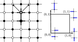
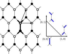
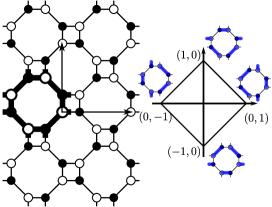
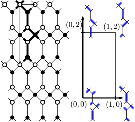
Figure 1. Some examples of $\mathbb{Z}^{2}$-periodic bipartite graphs (square, hexagon, square-octagon, square-hexagon) and their Newton polygons (cf. Theorem 2.3). The fundamental domain is indicated with thicker lines in the graph while the action of $\mathbb{Z}^{2}$ is represented by two arrows. Near each vertex of the Newton polygon is indicated the associated matching of the fundamental domain.

Note that there is a certain degree of arbitrariness in the embedding of $G$ in the plane and as a consequence a certain arbitrariness in the choice of the fundamental domain. For instance, in Fig. 1 the fundamental domain of $\mathbb{Z}^{2}$ contains two sites, but with a different embedding it could contain the four sites around a face (in this case the two axes of ${\mathbb{Z}}^{2}$ would be horizontal and vertical). In general, it is convenient to work with the smallest possible fundamental domain, as in Fig. 1.

A perfect matching of $G$ is a subset of edges, $M\subset E$, such that each vertex of $G$ is contained in one and exactly one edge in $M$. It is known that $G$ admits a matching (which is implicitly assumed from now on) if and only if $G_{1}$ does, and Fig. 1 shows that the fundamental domains of the four graphs we mentioned do admit several matchings. We denote $\Omega$ the set of matchings of $G$.

Assumption 1.

To avoid trivialities, we will assume that for every edge $e$ of $G$ there exists $M\in\Omega$ such that $e\in M$ and $M^{\prime}\in\Omega$ such that $e\notin M^{\prime}$ (one can easily construct pathological examples where this fails, but the edges in question can be simply removed and the matching problem is unchanged).

We will often refer to paths on the dual graph $G^{*}$:

Definition 2.1.

A path $\gamma$ on $G^{*}$ is a possibly infinite sequence $(\dots,f_{-1},f_{0},f_{1},\dots)$ of faces of $G$, such that $f_{i}$ is a neighbor of $f_{i+1}$. An infinite path $\gamma$ is called periodic if there exists a finite path $\gamma_{0}$ and $v\in{\mathbb{Z}}^{2}$ such that $\gamma$ is the concatenation of $\{T_{nv}\gamma_{0}\}_{n\in{\mathbb{Z}}}$, with $T_{v}$ the translation by $v$.

2.1.1. Height function and uniform measure

A flux is a function on the oriented edges of $G$, which is antisymmetric under the change of orientation of the edges. To each $M\in\Omega$ is associated a flux $\omega_{M}$: edges contained in $M$ carry unit flux, oriented from the white to the black vertex. Edges not contained in $M$ carry zero flux. Note that the divergence of $\omega_{M}$ is $1$ at white vertices and $-1$ at black vertices.

Fix now a reference matching $M_{0}$ (typically, a ${\mathbb{Z}}^{2}$-periodic matching, but the following definition would work for any flux of divergence $+1/-1$ at white/black vertices). $M_{0}$ allows to associate to $M$ a height function $h_{M}$ on $G^{*}$, as follows. Fix some face $f_{0}\in G^{*}$ (“the origin”) and set $h_{M}(f_{0})$ to some value, say $0$. For every $f\neq f_{0}$, let $\gamma$ be a path on $G^{*}$ starting at $f_{0}$ and ending at $f$. Then, $h_{M}(f)-h_{M}(f_{0})$ is the total flux of $\omega_{M}-\omega_{M_{0}}$ (say from right to left) across $\gamma$. Note that $h_{M}$ does not depend on the choice of the path (because $\omega_{M}-\omega_{M_{0}}$ has zero divergence) and that the height difference between two matchings $M,M^{\prime}$ is independent of the choice of the reference matching $M_{0}$.

In the following, the set of perfect matchings $\Omega$ will denote equivalently the set of all admissible height functions (it is understood that $M_{0}$ and $f_{0}$ are fixed). For lightness of notation, we will often write $h$ instead of $h_{M}$.

Definition 2.2.

Let $U$ be a simply connected open subset set of $[-1/2,1/2]^{2}$, $L>0$ and $U_{L}=L\,U$. We let $G^{\prime}$ be the finite subset of $G$ obtained by keeping all the vertices and edges belonging to faces which are entirely contained in $U_{L}$.

Given $m\in\Omega$ (called the “boundary condition”, with corresponding height function $h_{m}$) and $G^{\prime}=(E^{\prime},V^{\prime})$ as in Definition 2.2, let

$$\Omega_{m,G^{\prime}}=\left\{M\in\Omega:M|_{G\setminus G^{\prime}}=m|_{G\setminus G^{\prime}}\right\}$$ (2.1)

be the finite collection of matchings that coincide with $m$ outside of $G^{\prime}$. Equivalently, we can identify $\Omega_{m,G^{\prime}}$ as the set of height functions that coincide with $h_{m}$ except on the faces of $G^{\prime}$. We will implicitly assume (without loss of generality) that the reference face $f_{0}$ is not one of the faces of $G^{\prime}$. Clearly, $\Omega_{m,G^{\prime}}$ is non-empty (it includes at least $m$) and we will let $\pi_{m,G^{\prime}}$ denote the uniform measure over $\Omega_{m,G^{\prime}}$.

2.2. Pure phases

In this section we review known results about measures on the infinite graph $G$ whose typical height functions are close to a plane. First we will identify the set of “natural” measures of fixed average slope, then give a classification into three “phases” with very different correlation properties, and finally give their “microscopic” behavior, i.e. the probabilities of events depending on a finite subset of edges. Most results come from [12].

2.2.1. Ergodic Gibbs measure of fixed slope

Fix a reference matching $M_{0}$ assumed to be ${\mathbb{Z}}^{2}$-periodic. A measure $\mu$ on $\Omega$ is said to have slope $(s,t)$ if its expected height function is a linear function, with slope $(s,t)$: for all faces $f$, if $f^{\prime}$ denotes the translate of $f$ by $(x,y)\in{\mathbb{Z}}^{2}$, then $\mu[h(f^{\prime})-h(f)]=sx+ty$. $\mu$ is said to be a Gibbs measure if its conditional distributions on finite sub-graphs are uniform, $\mu(\,\cdot\,|M\in\Omega_{m,G^{\prime}})=\pi_{m,G^{\prime}}(\cdot)$ (DLR property). It is ergodic if it is not a linear combination of other Gibbs measures. Ergodic Gibbs measures of fixed slope can be thought of as the natural uniform measures on matchings of $G$ conditioned on their average slopes. The following theorem due to Sheffield [21] classifies all of them :

Theorem 2.3.

There exists a closed, convex polygon $N$ in ${\mathbb{R}}^{2}$ such that, for all $(s,t)$ in its interior $\stackrel{{\scriptstyle\raisebox{-2.0pt}[0.0pt][0.0pt]{ \scriptsize{$\circ$} }}}{{N}}$, there exists a unique ergodic Gibbs measure $\mu_{s,t}$ of slope $(s,t)$. The vertices of $N$ are determined by the slopes of some ${\mathbb{Z}}^{2}$-periodic matchings of $G$ (i.e. matchings of the fundamental domain) and thus are integer points. For $(s,t)\in\partial N:={N}\setminus\stackrel{{\scriptstyle\raisebox{-2.0pt}[0.0pt][0.0pt]{ \scriptsize{$\circ$} }}}{{N}}$, there exists an ergodic Gibbs measure but it may not be unique.

$N$ is called the Newton polygon, see Fig. 1.

2.2.2. Phase classification

As proved in [12], ergodic Gibbs measures come in three possible phases: solid, liquid and gas, depending on the position of $(s,t)$ in $N$.

• Solid phases correspond to slopes in $\partial N$. For any side $\ell$ of $\partial N$, there exists at least one infinite periodic path $\gamma$ on $G^{*}$ (cf. Definition 2.1) such that the configuration of the edges crossed by $\gamma$ (or by any of its translates) is deterministic and is the same for all measures with slope $(s,t)\in\ell$. The path $\gamma$ is said to be frozen.

  The asymptotic direction of $\gamma$ is determined as follows. All the planes with slope in $\ell$ and containing the origin of ${\mathbb{R}}^{3}$ intersect in a straight line. The direction of this line, when projected on the $(x,y)$ plane, is the direction of $\gamma$.

  At a vertex of the Newton polygon, which is the intersection of two sides of $\partial N$, there are two families of frozen paths with different directions, which form so to speak a grid on $G^{*}$. The components of the complement of the frozen paths are finite sets of faces. Heights are clearly independent in two distinct components, and the fluctuations of the height difference between two faces $f_{1},f_{2}$ are bounded deterministically and uniformly in the distance between them.

• Liquid phases correspond to generic points of $\stackrel{{\scriptstyle\raisebox{-2.0pt}[0.0pt][0.0pt]{ \scriptsize{$\circ$} }}}{{N}}$. In these phases, heights fluctuations behave like a Gaussian free field in the plane. In particular the variance of the height difference between $f_{1}$ and $f_{2}$ grows like $1/\pi$ times the logarithm of the distance, while edge correlations decay slowly (as the inverse of the square of the distance). Liquid phases are discussed in finer detail in the next section.

• Gaseous phases have exponentially decreasing edge correlations; the height difference fluctuations are not deterministically bounded, but their variance is bounded, uniformly with the distance of the faces. Gaseous phases may (but do not necessarily) occur when the slope $(s,t)$ is an integer point in $\stackrel{{\scriptstyle\raisebox{-2.0pt}[0.0pt][0.0pt]{ \scriptsize{$\circ$} }}}{{N}}$. The condition for the occurrence of a gaseous phase at an integer slope $(s,t)\in\stackrel{{\scriptstyle\raisebox{-2.0pt}[0.0pt][0.0pt]{ \scriptsize{$\circ$} }}}{{N}}$ is discussed in Section 2.3.

In the example of Fig. 1, only the square-octagon graph has a gaseous phase which has slope $(0,0)$.

2.2.3. Edge probabilities

When $(s,t)\in\stackrel{{\scriptstyle\raisebox{-2.0pt}[0.0pt][0.0pt]{ \scriptsize{$\circ$} }}}{{N}}$ (i.e. for liquid and gaseous phases) there is an explicit expression of edge probabilities under $\mu_{s,t}$.

Theorem 2.4.

[12] Fix $(s,t)\in\stackrel{{\scriptstyle\raisebox{-2.0pt}[0.0pt][0.0pt]{ \scriptsize{$\circ$} }}}{{N}}$. There exists an infinite periodic matrix $K_{s,t}=\{K_{s,t}({\rm w},{\rm b})\}_{{\rm w},{\rm b}}$ with ${\rm b}$ (resp. ${\rm w}$) ranging on black (resp. white) vertices of $G$ and an infinite periodic matrix $K_{s,t}^{-1}=\{K^{-1}_{s,t}({\rm b},{\rm w})\}_{{\rm w},{\rm b}}$ satisfying $K_{s,t}K^{-1}_{s,t}=Id$ such that, for any finite subset $\{e_{1}=({\rm w}_{1},{\rm b}_{1}),\ldots,e_{l}=({\rm w}_{l},{\rm b}_{l})\}$ of edges of $G$, the $\mu_{s,t}$-probability of seeing all of them occupied is:

$$\mu_{s,t}\bigl{(}e_{1}\in M,\dots,e_{l}\in M\bigr{)}=\Biggl{(}\prod_{j=1}^{l}K_{s,t}({\rm w}_{j},{\rm b}_{j})\Biggr{)}\det\bigl{(}K_{s,t}^{-1}({\rm b}_{k},{\rm w}_{i})\bigr{)}_{1\;\leqslant\;i,k\;\leqslant\;l}.$$

$K_{s,t}$ is called a Kasteleyn matrix. It is a weighted and signed version of the adjacency matrix, so in particular $K_{s,t}({\rm w},{\rm b})$ can be non-zero only if $({\rm b},{\rm w})$ is an edge of $G$. The signs (which are independent of the slope $(s,t)$) are chosen so that their product around any face $f$ is $-1$ if $f$ has $0\mod 4$ sides and $+1$ if it has $2\mod 4$ sides. We will not need to specify the explicit choice of signs, see [12]. Periodicity means that $K_{s,t}({\rm w}+(x,y),{\rm b}+(x,y))=K_{s,t}({\rm w},{\rm b})$ for every $(x,y)\in{\mathbb{Z}}^{2}$, and similarly for $K^{-1}_{s,t}$.

Given $K_{s,t}$ and two complex numbers $w,z$, we define a finite matrix ${\bf K}_{s,t}(z,w)$ from white to black vertices of the fundamental domain $G_{1}$, as follows. Consider $G_{1}$ as a weighted periodic bipartite graph on the torus, where the weight of an edge is the one induced by $K_{s,t}$, and note that it can contain multiple edges between two vertices, even if the infinite graph $G$ does not (see e.g. Fig. 1). Consider a path $\gamma_{x}$ (resp. $\gamma_{y}$) winding once horizontally (resp. vertically) along the torus and multiply by $z$ (resp. $1/z$) the weight of each edge crossed by $\gamma_{x}$ with the black vertex on the left (resp. on the right) and similarly by $w,1/w$ the edges crossed by $\gamma_{y}$. Then, ${\bf K}_{s,t}(z,w)$ is the adjacency matrix of $G_{1}$, with these modified weights. With the usual graph theory convention, this means that the $({\rm w},{\rm b})$ element of ${\bf K}_{s,t}(z,w)$ (with ${\rm w}$ (resp. ${\rm b}$) a white (resp. black) vertex of $G_{1}$) is the sum of the weights of the edges joining ${\rm w}$ to ${\rm b}$. Let $Q_{s,t}(z,w)$ (a matrix from black to white vertices of $G_{1}$) be the adjugate matrix of ${\bf K}_{s,t}(z,w)$ so that $[Q_{s,t}{\bf K}_{s,t}](z,w)=P(z,w)\text{Id}$ where $P(z,w)=\det({\bf K}_{s,t}(z,w))$. The $({\rm b},{\rm w})$ element of $Q_{s,t}(z,w)$ is denoted $Q^{{\rm b},{\rm w}}_{s,t}(z,w)$.

We can now give a formula for the inverse infinite Kasteleyn matrix $K_{s,t}^{-1}$:

Theorem 2.5.

[12] Let ${\rm b}$ and ${\rm w}$ be a black and a white vertex in $G_{1}$. The following holds for $(x,y)\in{\mathbb{Z}}^{2}$:

$$K_{s,t}^{-1}({\rm b},{\rm w}+(x,y))=\frac{1}{(2i\pi)^{2}}\int_{{\mathbb{T}}^{2}}\frac{Q^{{\rm b},{\rm w}}_{s,t}(z,w)}{P_{s,t}(z,w)}w^{x}z^{y}\frac{\mathrm{d}w}{w}\frac{\mathrm{d}z}{z}$$

where ${\mathbb{T}}^{2}=\{z,w\in{\mathrm{\hskip 1.99997pt\mathsf{l}C}}^{2},\lvert z\rvert=\lvert w\rvert=1\}$ is the unit complex torus.

Here, to avoid confusion, it can be useful to emphasize that $[Q_{s,t}/P_{s,t}](z,w)$ is the inverse of the finite matrix ${\bf K}_{s,t}(z,w)$, while $K_{s,t}^{-1}$ is an inverse of the infinite matrix $K_{s,t}$, with no dependence on $z,w$ (i.e. with the original edge weights).

2.3. Asymptotics of $K_{s,t}^{-1}$ and Gaussian fluctuations in the “liquid phase”

It is shown in [12] that, for an integer slope $(s,t)\in\stackrel{{\scriptstyle\raisebox{-2.0pt}[0.0pt][0.0pt]{ \scriptsize{$\circ$} }}}{{N}}\cap{\mathbb{Z}}^{2}$, the Laurent polynomial $P_{s,t}$ has either no zeros on the unit torus (in which case $\mu_{s,t}$ corresponds to a gaseous phase) or has a unique zero of order two (which corresponds to a liquid phase). For any non-integer slopes in $\stackrel{{\scriptstyle\raisebox{-2.0pt}[0.0pt][0.0pt]{ \scriptsize{$\circ$} }}}{{N}}\setminus{\mathbb{Z}}^{2}$, instead, $P_{s,t}$ has exactly two conjugate simple zeros. In this case Theorem 2.6 gives the asymptotics of $K_{s,t}^{-1}({\rm b},{\rm w})$ when the two vertices ${\rm b},{\rm w}$ are far apart. We emphasize that in our applications (i.e. in the proof of Theorem 2.8), we will have to consider only cases where the Newton polygon has no integer points in its interior.

Theorem 2.6.

[12] Fix $(s,t)$ a non-integer slope in $\stackrel{{\scriptstyle\raisebox{-2.0pt}[0.0pt][0.0pt]{ \scriptsize{$\circ$} }}}{{N}}$, so that $P_{s,t}$ has two simple zeros $(z_{0},w_{0})$ and $(\bar{z}_{0},\bar{w}_{0})$ on ${\mathbb{T}}^{2}$. Let $\alpha=\tfrac{\partial}{\partial z}P_{s,t}(z_{0},w_{0})$ and $\beta=\tfrac{\partial}{\partial w}P_{s,t}(z_{0},w_{0})$ and define $\phi(x,y)=x\alpha z_{0}-y\beta w_{0}$. Then the map $\phi:{\mathrm{IR}}^{2}\mapsto{\mathrm{\hskip 1.99997pt\mathsf{l}C}}$ is invertible, the matrix $Q_{s,t}(z_{0},w_{0})$ is of rank $1$ and can be written as $U_{s,t}V_{s,t}^{T}$ where the column vector $U_{s,t}$ (resp. $V_{s,t}$) is indexed by the black (resp. white) vertices of $G_{1}$. Moreover, we have

$$K^{-1}_{s,t}\bigl{(}{\rm b},{\rm w}+(x,y)\bigr{)}=-\Im\left(\frac{w_{0}^{x}z_{0}^{y}U_{s,t}({\rm b})V_{s,t}({\rm w})}{\pi\phi(x,y)}\right)+O\left(\frac{1}{x^{2}+y^{2}}\right)$$ (2.2)

where $O((x^{2}+y^{2})^{-1})$ has to be understood as $\frac{h(x,y)}{x^{2}+y^{2}+1}$ with $h$ bounded on ${\mathbb{Z}}^{2}$ and $\Im(z)$ denotes the imaginary part of $z$.

Remark 2.7.

The invertibility of $\phi$ is a consequence of the fact that $\alpha z_{0}$ is not collinear with $\beta w_{0}$. This is not proved explicitly in [12] but the argument is simple: Both the torus ${\mathbb{T}}^{2}$ and $P_{s,t}^{-1}(\{0\})$, the set of zeros of $P_{s,t}$, are two-dimensional manifolds in ${\mathrm{\hskip 1.99997pt\mathsf{l}C}}^{2}$ which contain $(z_{0},w_{0})$. The tangent space of ${\mathbb{T}}^{2}$ at $(z_{0},w_{0})$ is given by

$$p_{1}=\{a(iz_{0},0)+b(0,iw_{0})+(z_{0},w_{0}),(a,b)\in{\mathbb{R}}^{2}\}$$

and the tangent space of $P_{s,t}^{-1}(\{0\})$ is

$$p_{2}=\{\zeta(\beta,-\alpha)+(z_{0},w_{0}),\zeta\in{\mathrm{\hskip 1.99997pt\mathsf{l}C}}\}.$$

Since $(z_{0},w_{0})$ is a simple zero of $P_{s,t}$ seen as a function on ${\mathbb{T}}^{2}$, one necessarily has $p_{1}\cap p_{2}=\{(z_{0},w_{0})\}$ and it is easy to check that this fails if $\alpha z_{0}=\lambda\beta w_{0}$ with $\lambda\in{\mathbb{R}}$.

The asymptotic expression (2.2) is the main tool for the following result, that is proven in Appendix A:

Theorem 2.8.

Fix a non-integer slope $(s,t)\in\stackrel{{\scriptstyle\raisebox{-2.0pt}[0.0pt][0.0pt]{ \scriptsize{$\circ$} }}}{{N}}$ and $g\in G^{*}$. Under the Gibbs measure $\mu_{s,t}$, the moments of the variable

$$\frac{h(f)-h(g)-(\mu_{s,t}(h(f))-\mu_{s,t}(h(g)))}{\sqrt{{\operatorname{Var}}_{\mu_{s,t}}(h(f)-h(g))}}\sim\pi\;\frac{h(f)-h(g)-(\mu_{s,t}(h(f))-\mu_{s,t}(h(g)))}{\sqrt{\log|\phi(f)-\phi(g)|}}$$ (2.3)

tend as $|\phi(f)-\phi(g)|\to\infty$ to those of a standard Gaussian $\mathcal{N}(0,1)$.

Here and later, when we write $\phi(f)$ we mean $\phi(x,y)$ if $f$ is the $(x,y)$ translate of a face in the fundamental domain $G_{1}$. The fact that the variance of $h(f)-h(g)$ behaves like $(1/\pi^{2})\log|\phi(f)-\phi(g)|$ is proved in [12].

For the hexagonal lattice and under the assumption that $f$ and $f_{0}$ are along the same column of hexagons, convergence of the moments is proven in [8]. The general case is qualitatively more difficult and requires non-trivial work (see the discussion at the beginning of Appendix A; our proof uses ideas from [11, Sec. 7] but the setting here is more general and we give a more explicit control of the “error terms”).

2.4. Almost-planar boundary conditions

A central role will be played by “almost planar” boundary conditions.

We say that $h\in\Omega$ is an almost-planar height function with slope ${(s,t)}\in\stackrel{{\scriptstyle\raisebox{-2.0pt}[0.0pt][0.0pt]{ \scriptsize{$\circ$} }}}{{N}}$ if there exists $C$ such that, for every $f\in G^{*}$,

$$|h(f)-\mu_{s,t}(h(f))|\leq C.$$ (2.4)

We will sketch briefly in Section 2.5 a proof that almost-planar boundary conditions actually exist for every ${(s,t)}\in\stackrel{{\scriptstyle\raisebox{-2.0pt}[0.0pt][0.0pt]{ \scriptsize{$\circ$} }}}{{N}}$ (even with $C=1$).

Theorem 2.8 implies the following:

Theorem 2.9.

Fix a non-integer slope ${(s,t)}\in\stackrel{{\scriptstyle\raisebox{-2.0pt}[0.0pt][0.0pt]{ \scriptsize{$\circ$} }}}{{N}}$ and let $m$ be an almost-planar boundary condition with slope ${(s,t)}$. Let the finite graph $G^{\prime}$ be as in Definition 2.2. One has for every $\varepsilon>0$ and $n>0$:

$$\pi_{m,G^{\prime}}(\exists f\in G^{*}:|h(f)-\mu_{s,t}(h(f))|\geq L^{\varepsilon})=O(L^{-n}).$$ (2.5)

Remark 2.10.

The maximal equilibrium height fluctuation with respect to the average height should be of order $\log L$ with high probability, but we will not need such a refined result.

Proof of Theorem 2.9 given Theorem 2.8.

For the hexagonal lattice this is given in detail in [4] (see Proposition 4 there). For general graphs the proof is almost identical and we recall just the basic principle.

By monotonicity (see Section 3.1), the event $E_{f}=\{h(f)-\mu_{s,t}(h(f))\geq L^{\varepsilon}\}$ is more likely if we change the boundary condition for a higher one, i.e. if we replace $m$ with $m^{\prime}$ such that $h_{m^{\prime}}(f^{\prime})\geq h_{m}(f^{\prime})$ for every face $f^{\prime}\notin(G^{\prime})^{*}$ adjacent to some face in $(G^{\prime})^{*}$ (this set of faces is denoted here $\partial G^{\prime}$, and $(G^{\prime})^{*}$ is the collection of faces of $G^{\prime}$). Assume without loss of generality that the reference face $f_{0}$ where heights functions are fixed to zero belongs to $\partial G^{\prime}$. Then choose a random boundary condition $m^{\prime}$ from the measure $\mu_{s,t}$, and this time fix its height at the reference face as $h_{m^{\prime}}(f_{0})=h_{m}(f_{0})+L^{\varepsilon}/2=L^{\varepsilon}/2$. Thanks to Theorem 2.8, one has $h_{m^{\prime}}\geq h_{m}$ on $\partial G^{\prime}$, except with probability $O(L^{-n})$ for any given $n$. Finally, with such random boundary condition, by the DLR property the probability of $E_{f}$ is nothing but $\mu_{s,t}(h(f)-\mu_{s,t}(h(f))\geq L^{\varepsilon}/2)$, which is also $O(L^{-n})$, again thanks to Theorem 2.8. ∎

2.5. Perfect matchings, capacities and maximal configurations

2.5.1. Linear characterization of height functions

The set of height functions corresponding to a perfect matching of a finite subset of $G$ can be characterized by linear inequalities as follows.

Consider as in Definition 2.2 a finite sub-graph $G^{\prime}$ of $G$ and a boundary condition $m\in\Omega$. In this subsection we will use $m$ (even if it is not necessarily periodic) as reference matching for the definition of height functions. For any two neighboring faces $f,f^{\prime}$ with a common edge $e$ oriented positively (i.e. such that going from $f$ to $f^{\prime}$ one crosses $e$ leaving the white vertex on the right), let the oriented capacities $d(f,f^{\prime})$ and $d(f^{\prime},f)$ be defined as follows:

$$d(f,f^{\prime})=\begin{cases}0\text{ if }e\notin G^{\prime}\\ 0\text{ if }e\in G^{\prime}\text{ and }e\in m\\ 1\text{ if }e\in G^{\prime}\text{ and }e\notin m;\end{cases}\quad\quad d(f^{\prime},f)=\begin{cases}0\text{ if }e\notin G^{\prime}\\ 1\text{ if }e\in G^{\prime}\text{ and }e\in m\\ 0\text{ if }e\in G^{\prime}\text{ and }e\notin m\end{cases}.$$ (2.6)

Now for any pair of faces $f,f^{\prime}$ (not necessarily neighbors) let $D(f,f^{\prime})$ be the minimum over all paths $f=f_{1},\ldots,f_{n}=f^{\prime}$ in $G^{*}$ of the sum of the $d(f_{i},f_{i+1})$ (the minimum is well defined, the capacities being non-negative).

Proposition 2.11.

An integer-valued function $h$ on $G^{*}$ is the height function (with reference matching $m$) of a matching in $\Omega_{m,G^{\prime}}$ if and only if

$$\ D(f,f^{\prime})\;\geqslant\;h(f^{\prime})-h(f)\text{ for every }f,f^{\prime}\in G^{*}.$$ (2.7)

Proof.

The proof is in the spirit of [6, Theorem 1]. The “only if” part is trivial since, going back to Section 2.1.1, it is immediate to see that the maximal possible height difference $h(f^{\prime})-h(f)$ between neighboring faces $f,f^{\prime}$, for any matching in $\Omega_{m,G^{\prime}}$, does not exceed $d(f,f^{\prime})$. As for the “if” part, remark first of all that, thanks to (2.7), for every neighboring faces $f,f^{\prime}$ one has $h(f)-h(f^{\prime})\in\{-1,0,1\}$. Let us “mark” all edges $e\in G^{\prime}$ between faces $f,f^{\prime}$ (with $e$ oriented positively from $f$ to $f^{\prime}$) such that $h(f^{\prime})-h(f)=d(f,f^{\prime})$, together with edges $e\in G\setminus G^{\prime}$ such that $e\in m$. Let $M$ be the union of all marked edges and let us prove it is a matching (note that, automatically, $M\equiv m$ outside of $G^{\prime}$). For any white (resp. black) vertex $v$, let $e_{v}$ be the unique edge incident to $v$ which belongs to $m$. From (2.7) and considering paths that turn counterclockwise (resp. clockwise) around $v$, it is easy to see that:

• either all the faces $f$ sharing vertex $v$ have the same value of $h(f)$ and $e_{v}$ is the single marked edge around $v$;

• or there exists a single marked edge $e^{\prime}_{v}\neq e_{v}$, incident to $v$, such that $h(f^{\prime})=h(f)-1$, with $f,f^{\prime}$ neighboring faces sharing $e^{\prime}_{v}$, such that $v$ is on the left (resp. right) when going from $f$ to $f^{\prime}$.

$M$ is thus a matching and by construction $M\equiv m$ outside $G^{\prime}$. In conclusion, $M\in\Omega_{m,G^{\prime}}$ and of course its height function is just $h$. ∎

2.5.2. Maximal and minimal configurations

The characterization of height functions provided by Proposition 2.11 shows the existence of a unique maximal (resp. minimal) height function $h_{max}$ (resp. $h_{min}$) in $\Omega_{m,G^{\prime}}$. “Maximal” means that for any other height function $h$ in $\Omega_{m,G^{\prime}}$ satisfying $h(f_{0})=0$ (recall from Section 2.2 that the height is fixed to zero at some face $f_{0}$ outside of $G^{\prime}$) one has $h(f)\leq h_{max}(f)$ for every $f\in G^{*}$. Indeed, define $h_{max}(f):=D(f_{0},f)$ on $G^{*}$. This satisfies (2.7) (since $D(\cdot,\cdot)$ satisfies the triangular inequality) and maximality is a consequence of the fact that $d(f,f^{\prime})$ is the maximal possible height difference between neighboring faces. Similarly, one has $h_{min}(f)=-D(f,f_{0})$. Observe that the height functions $h_{max},h_{min}$ (with respect to the reference configuration $m$) vanish outside $G^{\prime}$ as they should (this is because the set of faces of $G$ not belonging to $G^{\prime}$ is connected, recall Definition 2.2).

2.5.3. Free paths and possible rotations

Definition 2.12.

Fix a matching $M\in\Omega$. We say that an oriented path $\gamma$ in $G^{*}$ is a free path (relative to $M$) if all edges crossed by $\gamma$ are free (i.e. not occupied) and have the same orientation (i.e. either all of them have their white vertex on the right of $\gamma$ or all of them on the left). If white vertices are on the right (resp. left) then $\gamma$ is called a positive (resp. negative) free path.

See Fig. 2.

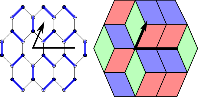
Figure 2. The relation between height function and dimer configuration in the case of the honeycomb graph. It is easy to see the right-hand drawing as a stepped surface in $3$ dimensions. It should be clear from the right-hand drawing that the positive free path (thick line) moves away at constant speed from the $(1,1,1)$ plane; at its endpoint (marked by an arrow) the free path cannot be possibly continued, and a cube can be added there (i.e. a rotation can be performed in the left-hand drawing).

A first observation is that free paths cannot form loops:

Proposition 2.13.

Let $\gamma$ be a free path relative to some $M\in\Omega$, and assume that $\gamma$ forms a simple loop. Then, for every $M^{\prime}\in\Omega$ the edges crossed by $\gamma$ are free.

Together with Assumption 1, this excludes loops.

Proof of Proposition 2.13.

Let $h$ be the height function of $M^{\prime}$, with reference matching $M$. Let $f$ be a face along $\gamma$. By symmetry, suppose $\gamma$ is a positive path. Since all edges are traversed with the positive orientation, we have

$$h(f)=h(f)+|\{\text{edges crossed by $\gamma$ and occupied in $M^{\prime}$}\}|$$

$$-|\{\text{edges crossed by $\gamma$ and occupied in $M$}\}|.$$

Since $\gamma$ crosses no occupied edge of $M$ by assumption, it crosses no occupied edge of $M^{\prime}$ either. ∎

A second observation is that, since only the reference matching (however it is chosen) makes a contribution to the height difference along a free path $\gamma$, the height function is non-increasing (resp. non-decreasing) if $\gamma$ is a positive (resp. negative) free path. An important consequence, that we will need in Section 4.2 to upper bound the equilibration time of the dynamics, is the following:

Proposition 2.14.

Fix $(s,t)\in\stackrel{{\scriptstyle\raisebox{-2.0pt}[0.0pt][0.0pt]{ \scriptsize{$\circ$} }}}{{N}}$. Let $M\in\Omega$ be such that the corresponding height function stays between two planes of slope $(s,t)$ and mutual distance $H$. All free paths relative to $M$ have length at most $CH$, where the constant $C$ depends only on $(s,t)$.

Proof of Proposition 2.14.

Since the graph $G$ is periodic, there exists only a finite number $k$ of types of faces that are not obtained by integer translation of each other. Let $\gamma$ be a positive free path (if it is a negative free path, the argument is similar) relative to some matching $M$. We claim that,

if one walks $$n \gamma f\mapsto h(f)-\mu_{s,t}(h(f))$$ steps along , the function decreases by at least (2.8)

$$-\lfloor n/k\rfloor\varepsilon \varepsilon=\varepsilon_{s,t}>0$$ for some .

Then, the proposition follows (with the constant $C$ being inversely proportional to $\varepsilon/k$) because the function $\mu_{s,t}(h(\cdot))$ on $G^{*}$ is essentially planar with slope $(s,t)$.

To prove (2.8), observe first that the matching $M$ gives no contribution to the variation of $h$ along $\gamma$ (all crossed edges are free) so that the variation of $h-\mu_{s,t}(h)$ is simply minus the $\mu_{s,t}$-average number of crossed edges which are covered by dimers. Fix some face $f\in\gamma$ and walk along $\gamma$ until a face $f^{\prime}$ which is a translate of $f$ is reached (the number of steps is at most $k$). The $\mu_{s,t}$-average of crossed dimers between $f$ and $f^{\prime}$ is non-negative and we will actually prove that it is strictly positive and independent of the type of face $f$, which implies the claim. Indeed, let $\tilde{\gamma}$ be the infinite periodic path on $G^{*}$ obtained by repeating periodically the finite portion of $\gamma$ which joins $f$ to $f^{\prime}$. If the average of crossed edges is zero, then clearly the slope of the height under the measure $\mu_{s,t}$ along the asymptotic direction of $\tilde{\gamma}$ is extremal, which contradicts the assumption that $(s,t)$ is in the interior of the Newton polygon $N$. Uniformity w.r.t. the type of the face $f$ is just a consequence of the fact that the number of different face types is finite. ∎

For any face $f$ of $G$, there exist exactly two ways to perfectly match its vertices among themselves. Label “$+$” one of the two matchings, and “$-$” the other (according to some arbitrary rule). If $M$ is a matching of $G$ such that the vertices of $f$ are matched only among themselves, we call “rotation around $f$” the transformation which consists in leaving $M$ unchanged outside of $f$, and in flipping from “$-$” to “$+$” (or vice-versa) the matching of the edges of $f$. If some vertices of $f$ are matched to vertices not belonging to $f$, then the rotation is not possible.

Free paths yield a way to find a face where an elementary rotation is possible. Given $M\in\Omega$, we pick an arbitrary face $f_{1}$ and we construct a growing sequence $\{\gamma_{n}\}_{n\geq 1}=\{(f_{1},\dots,f_{n})\}_{n\geq 1}$, of positive free paths, with $\gamma_{1}\equiv(f_{1})$ (an analogous construction gives a growing sequence of negative free paths). Given $\gamma_{n}$, consider all faces $f$ which are neighbors of $f_{n}$ and such that going from $f_{n}$ to $f$ one crosses a free edge with white vertex on the right. Choose $f_{n+1}$ (according to some arbitrary rule) among such faces. If there are no such faces available, we say that the procedure stops at step $n$. In this case, it means that every second edge around $f_{n}$ is occupied by a dimer, and this is exactly the condition so that a rotation at $f_{n}$ is possible. Altogether, we have proven:

Proposition 2.15.

Fix $(s,t)\in\stackrel{{\scriptstyle\raisebox{-2.0pt}[0.0pt][0.0pt]{ \scriptsize{$\circ$} }}}{{N}}$. Let $M\in\Omega$ be such that the corresponding height function stays between two planes of slope $(s,t)$ and mutual distance $H$. Within distance $C_{s,t}\,H$ from any face $f$ there exists a face $f^{+}$ (resp. $f^{-}$) where a rotation is possible; such a rotation increases (resp. decreases) the height at $f^{+}$ (resp. $f^{-}$) by $1$ and $h(f^{+})\;\leqslant\;h(f)\;\leqslant\;h(f^{-})$.

2.5.4. Almost planar height functions

Here we prove that almost-planar height functions satisfying (2.4) with $C=1$ do exist (under the assumption that $(s,t)\in\stackrel{{\scriptstyle\raisebox{-2.0pt}[0.0pt][0.0pt]{ \scriptsize{$\circ$} }}}{{N}}$ is a non-integer slope). Indeed from Theorem 2.8 and Borel-Cantelli we get that, for every fixed $\delta>0$, almost all configurations from $\mu_{s,t}$ satisfy

$$|h(f)-\mu_{s,t}(h(f))|\leq B+\delta|\phi(f)-\phi(f_{0})|$$ (2.9)

for some random $B$, where $f_{0}$ is the face where the heights are fixed to zero. Take one of these configurations. Let $A_{n}$ the set of faces at graph-distance at most $n$ from $f_{0}$ and suppose that $h(f)-\mu_{s,t}(h(f))<-1$ (the argument is similar if the difference is $>1$) for some $f\in A_{n}$. The same argument that led to Proposition 2.14 shows that, if $\delta$ is chosen small enough (say much smaller than the constant $\varepsilon_{s,t}$ in (2.8)), any positive free path $\gamma$ starting from $f$ is of length $O(\delta n/\varepsilon_{s,t})\leq n$ for $n$ large enough. Therefore, the last face $f^{\prime}$ of $\gamma$ is in $A_{2n}$ and (by the properties of positive free paths) one has $h(f^{\prime})-\mu_{s,t}(h(f^{\prime}))<-1$. By Proposition 2.15, a rotation is possible at $f^{\prime}$ and it increases $h(f^{\prime})-\mu_{s,t}(h(f^{\prime}))$ by $1$. The configuration thus obtained clearly still verifies (2.9) with the same $B$ and the quantity

$$\Delta=\sum_{f\in A_{2n}}|h(f)-\mu_{s,t}(h(f))|{\bf 1}_{|h(f)-\mu_{s,t}(h(f))|>1}$$

decreased by $1$. Since $\Delta$ is finite, the procedure can be repeated a finite number of times until there is no point left in $A_{n}$ with $|h(f)-\mu_{s,t}(h(f))|>1$. One concludes easily using the fact that $n$ can be taken arbitrarily large. ∎

3. Dynamics and mixing time

The dynamics we consider lives on the set $\Omega_{m,G^{\prime}}$ of matchings on a finite subset $G^{\prime}\subset G$ (as in Definition 2.2) with boundary condition $m\in\Omega$. Every face $f$ of $G^{\prime}$ has a mean-one, independent Poisson clock. When the clock at $f$ rings, if the rotation around $f$ is allowed, flip a fair coin: if “head” then choose the “$+$” matching of the edges of $f$, if “tail” then choose the “$-$” matching. In other words, perform the rotation around $f$ with probability $1/2$.

Call $\mu_{t}^{M}$ the law of the dynamics at time $t$, started from $M$.

Proposition 3.1.

For $t\to\infty$, $\mu_{t}^{M}$ converges to the uniform measure $\pi_{m,G^{\prime}}$.

Proof.

It is obvious that $\pi_{m,G^{\prime}}$ is invariant and reversible, so one should only check that the dynamics connects all the configurations in $\Omega_{m,G^{\prime}}$. This is done by using the free paths of Section 2.5.

Let $M\in\Omega_{m,G^{\prime}}$ and let $M_{max}\in\Omega_{m,G^{\prime}}$ be the matching corresponding to the maximal height function $h_{max}$ introduced in Section 2.5.2. The height function $h$ of $M$ with reference matching $M_{max}$ is clearly non-positive and vanishes outside $G^{\prime}$. Pick a face $f$ such as $h(f)\leq-1$ and consider a positive free path $\gamma$ growing from $f$ (as in the proof of Proposition 2.15). Along $\gamma$ the height function $h$ cannot grow and, $G^{\prime}$ being finite, $\gamma$ has to stop after a finite number of steps. The last face $f^{\prime}$ of $\gamma$ clearly is inside $G^{\prime}$ (since the height is zero outside) and we have already discussed that a rotation is possible at $f^{\prime}$ and it increases $h(f^{\prime})$ by $1$. By recursion, $M$ can be transformed into $M_{max}$ by a finite sequence of elementary rotations inside $G^{\prime}$. Arbitrariness of $M$ allows to conclude. ∎

As usual [16], an informative way to quantify the speed of approach to equilibrium is via the mixing time, defined as

$$T_{\rm mix}=T_{\rm mix}(m,G^{\prime})=\inf\{t>0:\max_{M\in\Omega_{m,G^{\prime}}}\|\mu_{t}^{M}-\pi_{m,G^{\prime}}\|<1/(2e)\}$$ (3.1)

where $\|\mu-\nu\|$ is the total variation distance of measures $\mu,\nu$ and the choice of the value $1/(2e)$ is conventional (any other value smaller than $1/2$ would do). With this choice, one has [16]

$$\max_{M\in\Omega_{m,G^{\prime}}}\|\mu_{t}^{M}-\pi_{m,G^{\prime}}\|\leq e^{-\lfloor t/T_{\rm mix}\rfloor}.$$ (3.2)

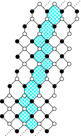
Figure 3. An example of the class of graphs where our results could be extended, see Remark 3.4. The shaded region is a thread (cf. Section 4.1). Layers of squares and hexagons can be of arbitrary vertical thickness and the periodicity in the “vertical” direction can be arbitrarily large.

We will study the mixing time when the boundary conditions are almost planar. The following is the main result of this work:

Theorem 3.2.

Fix $(s,t)\in\stackrel{{\scriptstyle\raisebox{-2.0pt}[0.0pt][0.0pt]{ \scriptsize{$\circ$} }}}{{N}}$, $m$ an almost-planar boundary condition of slope $(s,t)$ and let $G^{\prime}$ be as in Definition 2.2. If $G$ is either the square, hexagon or square-hexagon lattice (cf. Fig. 1) then there exists some $c>0$ such that

$$\quad\quad\quad\quad\quad\quad\quad\quad cL^{2}\leq T_{\rm mix}\leq L^{2+o(1)}.$$ (3.3)

We refer to Section 1.1.1 above for a discussion of previously known results.

Remark 3.3.

The proof of the lower bound in (3.3) actually shows the following: if the dynamics is started from the maximal configuration, which has an excess volume $c\,L^{3}$ with respect to the typical (almost flat) equilibrium configuration, it takes a time $c_{1}L^{2}$ before the excess volume becomes smaller than say $(c/2)\,L^{3}$ (which is still very large w.r.t. typical volume fluctuations). In this sense, the equilibration time lower bound is optimal.

Remark 3.4.

Our result could be extended to a class of graphs obtained by alternating periodically layers of squares and hexagons (see Fig. 3). On the other hand, we will explain in Section 5.1.3 why our method does not (and should not!) work for general periodic bipartite graphs $G$, in particular not for graphs like the square-octagon lattice which possesses a “gaseous phase”.

3.1. Monotonicity

It is natural to introduce the following partial order on $\Omega$ : $M\;\geqslant\;M^{\prime}$ if and only if $h_{M}(f)\;\geqslant\;h_{M^{\prime}}(f)$ for every $f\in G^{*}.$ As usual, the reference face $f_{0}$ is assumed to be fixed once and for all. Note that the partial order does not depend on the reference matching used to define the height. We say that an event $A\subset\Omega$ is increasing if $M\;\geqslant\;M^{\prime}$ and $M^{\prime}\in A$ implies $M\in A$. We define in the usual way stochastic domination: $\mu\succeq\mu^{\prime}$ if $\mu(A)\;\geqslant\;\mu^{\prime}(A)$ for every increasing event $A$.

Proposition 3.5.

The dynamics defined in Section 3 is monotone, that is $\mu_{t}^{M}\succeq\mu_{t}^{M^{\prime}}$ for every $t$ and every $M\geq M^{\prime}$.

Proof.

Couple the dynamics started from $M$ and $M^{\prime}$ by using the same clocks and the same coin tosses. Partial order is preserved along time. Indeed, it suffices to observe that if $h_{M}(f)=h_{M^{\prime}}(f)$ and a rotation at $f$ that increases the height by $1$ is possible for $M^{\prime}$, then necessarily the configuration of the edges of $f$ in $M$ is the same as in $M^{\prime}$, otherwise at some face $f^{\prime}$ neighboring $f$ one would have $h_{M}(f^{\prime})<h_{M^{\prime}}(f^{\prime})$. ∎

Remark 3.6.

As in [5, Sec. 2.2], one can realize all the evolutions $M_{t}^{M_{0}}$ for all possible initial conditions $M_{0}$ on the same probability space, with the property that if $M_{0}\leq M_{0}^{\prime}$ then almost surely $M_{t}^{M_{0}}\leq M_{t}^{M_{0}^{\prime}}$ for every $t\geq 0$. This construction is called global monotone coupling.

Proposition 3.7.

If $A$ is an increasing event, then $\pi_{m,G^{\prime}}(\cdot|A)\succeq\pi_{m,G^{\prime}}.$

Proof.

Remark that in the proof of Proposition 3.1 we showed that the maximal configuration can be reached from any other by a chain of rotations that increase the height, so $h_{\max}\in A$ and $A$ is connected. Consider the original dynamics started from $h_{\max}$ and the reflected dynamics (again started from $h_{\max}$) where each update that would leave $A$ is canceled. It is clear that they converge to $\pi_{m,G^{\prime}}$ and $\pi_{m,G^{\prime}}(\cdot|A)$ respectively and that, when coupled by using the same clocks and coin tosses, the second always dominates the first. ∎

Monotonicity allows to apply “censoring inequalities” of Peres and Winkler [18] which, roughly speaking, say the following: if the dynamics is started from the maximal or minimal configuration, deleting some updates along the evolution in a pre-assigned way (i.e. independently of the actual realization of the dynamics) increases the variation distance from equilibrium. The precise statement we need (cf. Corollary 3.9 below) is a bit more general than what is proven in [18] but the proof is almost identical, so we will just point out where some modification is needed.

Consider a probability measure $\pi$ on $\Omega$ and $P^{(v)},v\in\mathcal{V}$ a set of transition kernels that satisfy reversibility ($\pi(\sigma)P^{(v)}(\sigma\rightarrow\eta)=\pi(\eta)P^{(v)}(\eta\rightarrow\sigma)$) and monotonicity. We define a dynamics on $\Omega$ by assigning a Poisson clock of rate $c_{v}$ to each $v\in\mathcal{V}$ and applying $P^{(v)}$ when $v$ rings. The dynamics of Section 3 corresponds to $\mathcal{V}=(G^{\prime})^{*}$, $c_{v}=1$ and $P^{(f)}$ the kernel that corresponds to a rotation around $f$ with probability $1/2$ (if allowed).

Theorem 3.8.

Let $\nu_{0}$ be a probability measure on $\Omega$ such that $\frac{\mathrm{d}\nu_{0}}{\mathrm{d}\pi}$ is increasing. Consider $\nu_{t}$ the law at time $t$ of the dynamics started from $\nu_{0}$. Then, for every $t\geq 0$, $\frac{\mathrm{d}\nu_{t}}{\mathrm{d}\pi}$ is increasing and, if $\{\mu_{t}\}_{t\geq 0}$ is a family of probability measures such that $\nu_{t}\preceq\mu_{t}$ for all $t$, one has

$$\lVert\nu_{t}-\pi\rVert\;\leqslant\;\lVert\mu_{t}-\pi\rVert.$$

Corollary 3.9.

Let $\nu_{0}$ be as in Theorem 3.8. Suppose that for all $v\in\mathcal{V}$, for all $\nu$ such that $\frac{\mathrm{d}\nu}{\mathrm{d}\pi}$ is increasing, we have $P^{(v)}\nu\preceq\nu$. Let $\mu_{t}$ be the law at time $t$ of the dynamics started from $\nu_{0}$, where the rates $c_{v}$ of the Poisson clocks are replaced by deterministic time-dependent rates $\tilde{c}_{v}(s)$, such that $0\leq\tilde{c}_{v}(s)\leq c_{v}$ for every $0\leq s\leq t$. Then,

$$\text{for every }t\geq 0,\quad\nu_{t}\preceq\mu_{t}\text{ and }\lVert\nu_{t}-\pi\rVert\;\leqslant\;\lVert\mu_{t}-\pi\rVert.$$

Remark 3.10.

The hypothesis of ${\mathrm{d}\nu_{0}}/{\mathrm{d}\pi}$ increasing is immediate if the dynamics is started from the maximal configuration $h_{\max}$, since in that case $\nu_{0}$ is concentrated on $h_{max}$.

As in [18], the proof of Theorem 3.8 follows directly from the following two lemmas.

Lemma 3.11.

With the above definitions, for any probability measure $\mu$, if $\frac{\mathrm{d}\mu}{\mathrm{d}\pi}$ is increasing then $\frac{\mathrm{d}P^{(v)}\mu}{\mathrm{d}\pi}$ is increasing.

This replaces Lemma 2.1 of [18], which uses explicitly the fact that the dynamics is of “heat-bath” type.

Proof.

$$\frac{\mathrm{d}P^{(v)}\mu}{\mathrm{d}\pi}(\sigma) =\frac{1}{\pi(\sigma)}\sum_{s}\mu(s)P^{(v)}(s\rightarrow\sigma)=\frac{1}{\pi(\sigma)}\sum_{s}\frac{\mu(s)}{\pi(s)}\pi(s)P^{(v)}(s\rightarrow\sigma)$$ (3.4)

$$=\frac{1}{\pi(\sigma)}\sum_{s}\frac{\mu(s)}{\pi(s)}\pi(\sigma)P^{(v)}(\sigma\rightarrow s)={\mathbb{E}}^{(v)}_{\sigma}\bigl{[}\frac{\mathrm{d}\mu}{\mathrm{d}\pi}(X)\bigr{]}$$ (3.5)

where $X$ is the state after one action of $P^{(v)}$, starting from $\sigma$. The third equality uses the reversibility and the monotonicity of $P^{(v)}$ shows that the last expression is increasing in $\sigma$. ∎

Lemma 3.12.

[18, Lemma 2.4] If $\mu$, $\nu$ are two probability measures on $\Omega$ such that $\frac{\mathrm{d}\nu}{\mathrm{d}\pi}$ is increasing and $\nu\preceq\mu$, then $\lVert\nu-\pi\rVert\;\leqslant\;\lVert\mu-\pi\rVert$.

Proof of Corollary 3.9.

Decompose the Poisson point process (PPP) of density $c_{v}$ on $\mathbb{R}^{+}$ as the union of two independent PPPs, $X$ and $Y$, of non-constant densities $\tilde{c}_{v}(s)$ and $c_{v}-\tilde{c}_{v}(s)\geq 0$. The dynamics $\mu_{t}$ is obtained by erasing the updates from the process $Y$. From Lemma 3.11 we get that $\frac{\mathrm{d}\nu_{t}}{\mathrm{d}\pi}$ is increasing. Censoring an update $P^{(v)}$ at time $t$ conserves the stochastic domination because, by induction, $\nu_{t}=P^{(v)}\nu_{t^{-}}\preceq\nu_{t^{-}}\preceq\mu_{t^{-}}=\mu_{t}$. ∎

4. Mapping to a “bead model”

4.1. From dimers to “beads”

From this point onward, we will assume that the graph $G$ is either the square, hexagon or square-hexagon graph (see Fig. 1) since we will use some of their geometric properties.

The set $\Omega$ of matchings of $G$ can be mapped into the configurations of what we call a bead model. Such a correspondence is valid for more general graphs than the square, hexagon and square-hexagon, provided that the graph in question possesses a certain “fibration” with fibers (or threads) satisfying the properties described below. See Remark 3.4 for a more general class of graphs where this construction would work.

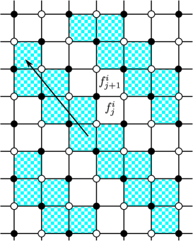
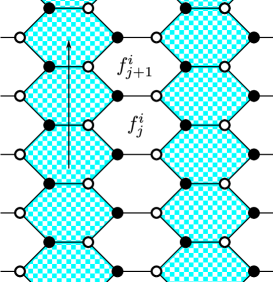
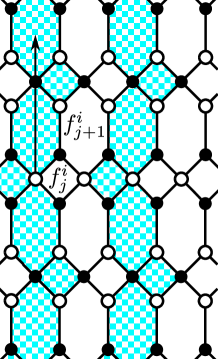
Figure 4. The paths called threads and used in the definition of the bead model for the square, hexagon and square hexagon graph. The arrow shows the orientation of the threads.

As is apparent from Fig. 4, for the three types of graph we are considering, there exists a family of directed periodic paths $\{\gamma_{i}\}_{i\in{\mathbb{Z}}}$ (called threads) on $G^{*}$ such that

1. labeling the faces along thread $\gamma_{i}$ as $\{f^{i}_{j}\}_{j\in{\mathbb{Z}}}$, face $f^{i}_{j}$ neighbors only $f^{i}_{j\pm 1}$ and some faces of $\gamma_{i\pm 1}$;

2. going from the face $f^{i}_{j}$ to $f^{i}_{j+1}$, one crosses an edge of $G$ (call it $e^{i}_{j}$) which is positively orientated. Such edges are called transverse edges and dimers on transverse edges are called beads;

3. threads $\gamma_{i}$ are obtained one from the other by a suitable ${\mathbb{Z}}^{2}$ translation and $\cup_{i}\gamma_{i}=G^{*}$.

Proposition 4.1.

Consider a finite sub-graph $G^{\prime}\subset G$ as in Definition 2.2 (recall that $G\setminus G^{\prime}$ is connected) and a boundary condition $m\in\Omega$. A matching in $\Omega_{m,G^{\prime}}$ is uniquely determined by the position of its beads. Furthermore the number of beads in $G^{\prime}$ on each thread $\gamma_{i}$ is the same for every $M\in\Omega_{m,G^{\prime}}$.

Proof.

From the definition of height function and using property (ii) above of threads, which says that transverse edges are all crossed with the same orientation, the height at some $f\in(G^{\prime})^{*}$ belonging to thread $\gamma_{i}$ is determined by the number of beads on $\gamma_{i}$ between the boundary of $G^{\prime}$ and $f$. Hence the position of beads uniquely determines the height function and thus the matching. The total number of beads on $\gamma_{i}\cap(G^{\prime})^{*}$ is determined by the height difference between two faces $f_{1},f_{2}$ of $\gamma_{i}\setminus(G^{\prime})^{*}$, such that the portion of $\gamma_{i}$ between $f_{1}$ and $f_{2}$ includes $\gamma_{i}\cap(G^{\prime})^{*}$. This height difference is clearly independent of the particular chosen matching in $\Omega_{m,G^{\prime}}$ (because $f_{1},f_{2}$ are outside $G^{\prime}$ and $G\setminus G^{\prime}$ is connected). ∎

In order to have a complete picture, we have to determine the condition for a set of beads’ positions to correspond to a matching of $G$, that is the kind of constraints beads impose on each other. We first need some notations (see Fig. 5).

Definition 4.2.

Let as above $e^{i}_{j}$ denote the $j^{\text{th}}$ transverse edge of the thread $\gamma_{i}$ and let ${\rm b}_{j}^{i}$ (resp. ${\rm w}_{j}^{i}$) denote its black (resp. white) vertex. Let $\Gamma^{i}$ be the set of vertices of $G$ which belong both to $\gamma_{i}$ and to $\gamma_{i+1}$, and order vertices in $\Gamma^{i}$ following the same direction as for the faces along the threads. Note that $\Gamma^{i}$ contains the white vertices of transverse edges of $\gamma_{i}$ and the black vertices of transverse edges of $\gamma_{i+1}$. Given transverse edges $e^{i}_{j},e^{i+1}_{j^{\prime}}$ on $\gamma_{i},\gamma_{i+1}$, we write $e^{i}_{j}\prec e_{j^{\prime}}^{i+1}$ (resp $e^{i}_{j}\succ e_{j^{\prime}}^{i+1}$) if ${\rm w}_{j}^{i}$ is below (resp. above) ${\rm b}_{j^{\prime}}^{i+1}$.

Proposition 4.3.

A set of bead positions corresponds to a matching in $\Omega$ if and only if, for any two consecutive beads on the same thread (i.e. beads on transverse edges $e^{i}_{a},e^{i}_{b},a<b$ with no bead between them along the same thread $\gamma_{i}$), there is a unique bead in thread $\gamma_{i-1}$ and a unique bead in thread $\gamma_{i+1}$ such that their positions $e^{i-1}_{c},e^{i+1}_{d}$ satisfy $e^{i}_{a}\prec e^{i-1}_{c}\prec e^{i}_{b}$ and $e^{i}_{a}\prec e^{i+1}_{d}\prec e^{i}_{b}$.

Proof. We advise the reader to keep an eye on Fig. 5 while reading this proof.

Proof of the “only if” part. Without loss of generality we can consider threads $\gamma_{i}$ and $\gamma_{i+1}$. Note that following $\Gamma^{i}$ between ${\rm w}^{i}_{a}$ and ${\rm w}^{i}_{b}$ there is necessarily exactly one more black vertex than white vertex (because $G$ is bipartite). Since by assumption there are no beads on $\gamma_{i}$ between $e^{i}_{a}$ and $e^{i}_{b}$, all the white vertices have to be matched within $\Gamma^{i}$. This leaves exactly a single black vertex which has to be matched along a transverse edge in $\gamma_{i+1}$. The corresponding dimer is the unique bead such that its position $e^{i+1}_{d}$ satisfies $e^{i}_{a}\prec e^{i+1}_{d}\prec e^{i}_{b}$.

Proof of the “if” part. Suppose that the bead positions are given and that they satisfy the properties above. This automatically fixes which transverse edges are occupied and which are free. To see that the rest of the matching is also (uniquely) determined, proceed as follows. With the same notations as above, consider the vertices of $\Gamma^{i}$ between ${\rm w}^{i}_{b}$ and ${\rm b}^{i+1}_{d}$. These vertices are all matched with each other (because by construction $e^{i+1}_{d}$ is the “highest” bead in $\gamma_{i+1}$ such that $e^{i+1}_{d}\prec e^{i}_{b}$) and they form a path with an equal number of alternating white and black vertices, so there is a unique way of matching them. The same goes for vertices between ${\rm w}^{i}_{a}$ and ${\rm b}^{i+1}_{d}$. ∎

Remark 4.4.

Fix $G^{\prime}\subset G$ and a boundary condition $m\in\Omega$. Under the measure $\pi_{m,G^{\prime}}$, conditionally on the positions of the beads in $\gamma_{i\pm 1}$, the beads of $\gamma_{i}$ are independent and each has a uniform distribution in a certain finite set of adjacent transverse edges (two transverse edges being adjacent if they are of the form $e^{i}_{j},e^{i}_{j+1}$; remark that on the square lattice they can actually share a vertex, while on the hexagonal lattice they cannot). Indeed, given a bead on the transverse edge $e^{i}_{a}$, it is possible to move it up to $e^{i}_{a+1}$ (resp. down to $e^{i}_{a-1}$) via a rotation of the face $f^{i}_{a+1}$ (resp. $f^{i}_{a}$), provided that $f^{i}_{a+1}$ (resp. $f^{i}_{a}$) is within $G^{\prime}$ and that the new position does not violate the ordering properties of Proposition 4.3. Uniformity of the distribution is trivial from uniformity of the unconditional measure $\pi_{m,G^{\prime}}$. Note also that moving a bead up (resp. down) implies changing by $-1$ (resp. $+1$) the height of the face just above (below) it along the thread.

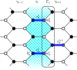
Figure 5. An example of the situation in the proof of proposition 4.3. Beads on the edges $e_{a}^{i}$ and $e_{b}^{i}$ are indicated by thick lines.

4.2. Dynamics in terms of beads

The Glauber dynamics defined in Section 3 has a simple interpretation in terms of the bead model. As observed in Remark 4.4, a rotation is equivalent to moving a bead to an adjacent transverse edge in the same thread (in particular, rotations are possible only at faces adjacent to a bead, and the configuration of beads outside $G^{\prime}$ is frozen). We can then redefine the dynamics as follows. Each bead in $G^{\prime}$ has a mean-one independent Poisson clock; when it rings, with probabilities $1/2,1/2$ move the bead either up or down to the adjacent transverse edge if allowed by the boundary conditions and by the ordering properties.

4.2.1. Fast dynamics

As mentioned in the introduction, we will not work directly with the original Glauber dynamics but rather with an auxiliary one. We will actually need two auxiliary dynamics: one, that we call synchronous fast dynamics, will be useful to upper bound the mixing time, while the asynchronous fast dynamics will provide a lower bound.

Definition 4.5.

1. We define the synchronous fast dynamics as follows. We have two independent mean-1 Poisson clocks. When the first (resp. second) one rings we resample all the bead positions on even-labelled (resp. odd-labelled) threads following the equilibrium measure $\pi_{m,G^{\prime}}$ conditioned on the state of beads on odd (resp. even) threads.

2. The asynchronous fast dynamics is defined instead by giving each bead in $G^{\prime}$ an independent mean-1 Poisson clock. When a clock rings, the position of the corresponding bead is resampled from $\pi_{m,G^{\prime}}$ conditioned on the position of all other beads. Note that, by construction, beads outside $G^{\prime}$ are frozen.

Thanks to monotonicity of the original Glauber dynamics, one sees easily that both synchronous and asynchronous fast dynamics are monotone.

Remark 4.6.

Recall Remark 4.4: the positions accessible to a single bead, given the beads of neighboring threads and the boundary conditions, form a segment of the transverse edges of its thread and these segments are mutually non-intersecting. Thus, under both synchronous and asynchronous dynamics each bead is resampled with the uniform law on a finite segment.

4.2.2. Comparisons of mixing times, and constrained dynamics

As announced, the asynchronous dynamics will provide a mixing time lower bound for the original one.

Proposition 4.7.

Fix $G^{\prime}\subset G$ as in Definition 2.2 and a boundary condition $m$, not necessarily almost planar. Let $T_{\rm mix}$ be the mixing time for the original dynamics and let $T^{a}$ be the first time such that the law of the asynchronous dynamics, started from the maximal configuration, is within variation distance $1/(2e)$ from equilibrium. Then, $T_{\rm mix}\geq T^{a}$.

Proof.

Recall the definition (3.1) of mixing time: to get a lower bound, we can just look at the evolution from the maximal configuration $h_{max}$, which we can therefore assume to be the initial configuration of both original and asynchronous fast dynamics. From the description of the asynchronous fast dynamics in Section 4.2.1, we see that we can couple the two dynamics using the same Poisson clocks for each bead. To prove that the asynchronous dynamics approaches equilibrium faster than the original one it is enough to show that if $\frac{\mathrm{d}\nu}{\mathrm{d}\pi}$ is increasing then, writing $P^{(b)}$ and $\tilde{P}^{(b)}$ for the kernels corresponding to an update of the bead $b$ according to the original and asynchronous fast dynamics respectively, one has

$$\tilde{P}^{(b)}\nu\preceq P^{(b)}\nu.$$ (4.1)

Indeed, together with monotonicity this guarantees that the height function is stochastically lower under the asynchronous dynamics than under the original one and then Theorem 3.8 can be applied (with $\mu_{t}$ the law of the original dynamics and $\nu_{t}$ that of the asynchronous one).

By conditioning on all the beads except $b$, we can assume that $\nu$ is a measure on some interval $\{0,\ldots,k\}$ and that $\pi$ is the uniform measure on the same interval (cf. Remark 4.4) in which case it is trivial to check (4.1). Indeed, $\tilde{P}^{(b)}\nu=\pi$ for every $\nu$, and $\mathrm{d}P^{(b)}\nu/\mathrm{d}\pi$ is increasing (cf. Lemma 3.11 and recall the assumption $\mathrm{d}\nu/\mathrm{d}\pi$ increasing), which implies $\pi\preceq P^{(b)}\nu$. ∎

4.2.3. Constrained dynamics

Next, we bound $T_{\rm mix}$ from above using the synchronous dynamics: this works well only if the dynamics is constrained between two configurations whose height functions are not too different. Given two matchings $M_{-}\leq M_{+}$ in $\Omega_{m,G^{\prime}}$ ($M_{-}$ will be called “the floor” and $M_{+}$ “the ceiling”) the constrained dynamics is defined in the subset $\Omega^{M_{\pm}}_{m,G^{\prime}}\subset\Omega_{m,G^{\prime}}$ such that $M_{-}\leq M\leq M_{+}$: it is obtained from the original dynamics, erasing all updates which would exit $\Omega^{M_{\pm}}_{m,G^{\prime}}$. It is elementary to check that monotonicity still holds, and the equilibrium measure is of course $\pi_{m,G^{\prime}}^{M_{\pm}}:=\pi_{m,G^{\prime}}(\cdot|M_{-}\leq\cdot\leq M_{+})$. The distance between floor and ceiling is defined as $H=\max_{f\in G^{*}}(h_{M_{+}}(f)-h_{M_{-}}(f))$. To avoid a proliferation of notations, we still call $T_{\rm mix}$ the mixing time of the dynamics constrained between $M_{-}$ and $M_{+}$, and $\mu_{t}^{M}$ its law at time $t$, with initial condition $M$.

To estimate $T_{\rm mix}$ within logarithmic multiplicative errors, we can restrict ourselves to the evolution started from the extreme configurations (see for instance [5, Eq. (6.5)]):

Lemma 4.8.

Consider the dynamics constrained between $M_{-}$ and $M_{+}$. For any $t>0$ and any $M\in\Omega_{m,G^{\prime}}^{M_{\pm}}$,

$$\lVert\mu_{t}^{M}-\pi_{m,G^{\prime}}^{M_{\pm}}\rVert\;\leqslant\;2H\lvert(G^{\prime})^{*}\rvert\max\left[\lVert\mu_{t}^{M_{+}}-\pi_{m,G^{\prime}}^{M_{\pm}}\rVert,\lVert\mu_{t}^{M_{-}}-\pi_{m,G^{\prime}}^{M_{\pm}}\rVert\right]$$

with $\lvert(G^{\prime})^{*}\rvert$ the number of faces of $G^{\prime}$.

In the next result, $T_{\rm mix}^{s}$ denotes the mixing time of the synchronous dynamics constrained between $M_{-}$ and $M_{+}$ (just take the Definition 4.5 of the synchronous dynamics and replace $\pi_{m,G^{\prime}}$ by $\pi^{M_{\pm}}_{m,G^{\prime}}$ there):

Proposition 4.9.

Fix $G^{\prime}\subset G$ as in Definition 2.2 and boundary condition $m$. Suppose $m$ is almost planar with slope $(s,t)\in\stackrel{{\scriptstyle\raisebox{-2.0pt}[0.0pt][0.0pt]{ \scriptsize{$\circ$} }}}{{N}}$ and consider floor/ceiling $M_{\pm}\in\Omega_{m,G^{\prime}}$, at distance $H$ from each other. We have

$$T_{\rm mix}\;\leqslant\;\bigl{(}C_{s,t}H^{2}\log^{3}(H\lvert(G^{\prime})^{*}\rvert)\bigr{)}T_{\rm mix}^{s}.$$

Proof.

A complete proof for the hexagonal graph is given in [4, Section 6.2] and since for the square or square-hexagon graph not much changes, we will be somewhat sketchy.

For simplicity we will write $\pi$ for $\pi_{m,G^{\prime}}^{M_{\pm}}$. One first proves that a single update of the synchronous fast dynamics can be realized by letting the original dynamics evolve for a time $O(H^{2}(\log H)(\log\lvert(G^{\prime})^{*}\rvert))$ while censoring some updates. Indeed, consider the dynamics obtained by starting from $M$ and setting to $0$ the rate of updates of beads on, say, odd threads in the original dynamics. It is clear that this auxiliary evolution converges to the uniform measure on configurations of beads on even thread conditioned by the beads on odd threads, which is exactly the measure after one “even update” of the synchronous fast dynamics, and Remark 4.6 allows us to easily compute its mixing time. Beads on odd threads are frozen and those on even threads are completely independent so we have to compute the mixing time for a set of independent one-dimensional simple random walks on domains of the type $\{0,\ldots,k_{i}\}$. By Proposition 2.14 the $k_{i}$ are bounded by $C_{s,t}H$ (because, if a bead can be moved $n$ steps up, necessarily there is a length-$n$ free path along the thread) so the mixing time for each walk is $O(H^{2}\log H)$ and for $O(\lvert(G^{\prime})^{*}\rvert)$ such walks it becomes $O(H^{2}(\log H)(\log\lvert(G^{\prime})^{*}\rvert))$.

It is then clear that the law of the synchronous fast dynamics at time $t$, call it $\nu_{t}^{M}$, coincides (except for a negligible total variation error term), with that of the original dynamics at time $n(t)\Delta$ after censoring suitable updates, where

$$\Delta=C_{s,t}H^{2}(\log H)(\log\lvert(G^{\prime})^{*}\rvert)\leq C_{s,t}H^{2}\log^{2}(H|(G^{\prime})^{*}|)$$

and $n(t)$ is a Poisson random variable of average $2t$ (this is the number of updates within time $t$ for the synchronous dynamics). Since we will take $t$ large, we can replace $n(t)$ with its average (we skip details). If Corollary 3.9 is applicable (see below), we obtain then that $\lVert\mu^{M_{\pm}}_{2t\Delta}-\pi\rVert\leq\lVert\nu^{M_{\pm}}_{t}-\pi\rVert.$ Then, using Lemma 4.8 and (3.2),

$$\sup_{M}\lVert\mu^{M}_{2A\Delta T_{\rm mix}^{s}}-\pi\rVert\leq 2H|(G^{\prime})^{*}|\max\left[\lVert\mu_{2A\Delta T_{\rm mix}^{s}}^{M_{+}}-\pi\rVert,\lVert\mu_{2A\Delta T_{\rm mix}^{s}}^{M_{-}}-\pi\rVert\right]$$ (4.2)

$$\leq 2H|(G^{\prime})^{*}|\max\left[\lVert\nu^{M_{+}}_{AT_{\rm mix}^{s}}-\pi\rVert,\lVert\nu^{M_{-}}_{AT_{\rm mix}^{s}}-\pi\rVert\right]\leq 2H|(G^{\prime})^{*}|e^{-\lfloor A\rfloor}$$ (4.3)

which is smaller than $1/(2e)$ for some $A$ of order $\log(H|(G^{\prime})^{*}|)$.

To see that Corollary 3.9 is applicable, we have to check that ${\mathrm{d}\mu}/{\mathrm{d}\pi}$ increasing implies $P^{(b)}\mu\preceq\mu$ with $P^{(b)}$ the kernel of the update of bead $b$ under the original dynamics, where beads move by $\pm 1$ along their respective thread. Conditioning on all other beads, we can assume that $\mu$ is a probability on an interval $\{0,\dots,k\}$ and that $\pi$ is the uniform measure on the same interval. Then, summation by parts shows that

$$P^{(b)}\mu(f)-\mu(f)=-\frac{1}{2}\sum_{x=1}^{k}[\mu(x)-\mu(x-1)][f(x)-f(x-1)]$$

which is negative if $f$ is increasing ($\mu$ is also increasing). ∎

4.2.4. Volume drift

In this section we study the time evolution of the volume between two configurations under the (a)synchronous fast dynamics. This will be the key to evaluate their mixing time and thus, thanks to Propositions 4.7 and 4.9, the mixing time of the original dynamics. Note that in Proposition 4.10 we do not require the boundary condition to be almost-planar.

Proposition 4.10.

Let $M^{1},M^{2}\in\Omega_{m,G^{\prime}}$ be such that $M^{1}\;\leqslant\;M^{2}$ and let $M^{i}_{t},i=1,2$ denote the evolution starting from $M^{i}$ and following the fast dynamics (synchronous or asynchronous: we use the same notation). Letting $\mathcal{F}_{t}$ denote the filtration induced by $\{M^{i}_{s},i=1,2,s\leq t\}$ and $V_{t}=\sum_{f\in G^{*}}[h_{M^{2}_{t}}(f)-h_{M^{1}_{t}}(f)]$, then $V_{t}$ is a supermartingale:

$$\mathbb{E}\bigl{[}V_{t}|\mathcal{F}_{t^{\prime}}\bigr{]}\;\leqslant\;V_{t^{\prime}}\text{ for every }t\geq t^{\prime}.$$

The same holds if the fast dynamics is constrained between a floor $M_{-}$ and a ceiling $M_{+}$.

Note that, since the volume is expressed as a sum of height differences, it does not matter whether $M_{t}^{1}$ evolves independently of $M^{2}_{t}$ or not.

Proof.

First of all note that the expected drift

$$\lim_{\varepsilon\searrow 0}\frac{1}{\varepsilon}[{\mathbb{E}}(V_{\varepsilon})-V_{0}]$$ (4.4)

is the same for the synchronous and for the asynchronous fast dynamics (as a function of the initial conditions $M^{1},M^{2}$): this is thanks to the fact that the volume is a sum of height differences over faces, that expectation is linear and that beads in the same thread are updated independently in a step of the synchronous dynamics. (This does not imply that the process $V_{t}$ itself or even its average is the same for the two dynamics). In the following, we will therefore assume that we deal with the synchronous dynamics and prove that (4.4) is not positive.

From the proof of Proposition 3.1, we see that there exists a sequence of configurations $M_{(0)},\dots,M_{(k)}$ such that $M_{(0)}=M^{2},M_{(k)}=M^{1}$ and $M_{(i)}$ is obtained by $M_{(i-1)}$ via a rotation that decreases the height at some face $f$. Writing the volume difference between $M^{2}$ and $M^{1}$ as a telescopic sum of volume differences between $M_{(i)}$ and $M_{(i-1)}$ and using linearity of the expectation, we see that to prove (4.4) we can restrict to the case where $M^{1}$ and $M^{2}$ differ only by a rotation on a single face $f$. We will actually prove that the expected change of $V$ from a single update is $0$ except when $f$ is suitably close to the boundary of $G^{\prime}$, in which case it can be negative (see Remark 4.11 for a more precise discussion).

The proof will be given only for the square-hexagon graph since it contains all the difficulties, but the same method works equally well for the hexagon or square graph.

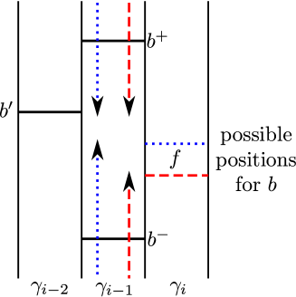
(a) (b)

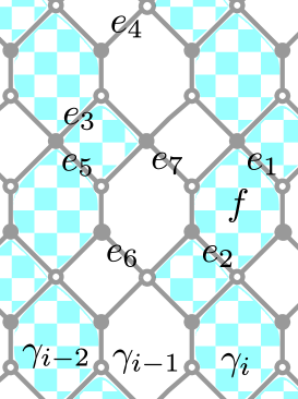
Figure 6. Volume drift when $f$ is a hexagon. (a): a schematic representation of threads $\gamma_{i},\gamma_{i-1},\gamma_{i-2}$ with the beads $b,b^{\pm},b^{\prime}$. (b): a more detailed view of the three threads in question, with the hexagonal face $f$ and the transverse edges $e_{1},\dots,e_{7}$ mentioned in the proof.

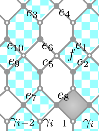
Figure 7. Volume drift when $f$ is a square. The threads $\gamma_{i},\gamma_{i-1},\gamma_{i-2}$ with the face $f$ and the transverse edges $e_{i},i=1,\dots,10$. A square face like $f$, which is adjacent to hexagons of the thread to its left, is called a “Type I” square, while a square like the shaded one (adjacent to hexagons of the thread to its right) is called “Type II”. Note that if $f$ were a Type II square say again on $\gamma_{i}$, then by symmetry $\gamma_{i-1}$ would not contribute to the volume change but the thread $\gamma_{i+1}$ would.

Case 1: $f$ is a hexagon. Suppose that the face $f$, whose rotation brings $M^{1}$ to $M^{2}$, is a hexagon on thread $\gamma_{i}$ (cf. Fig. 6). Then, there is a certain bead $b$ which in the two configurations is on two different adjacent transverse edges of $\gamma_{i}$ on the boundary of $f$ (such edges are called $e_{1}$ and $e_{2}$ in the picture). Now consider a step of the synchronous dynamics. If threads with the same parity as $\gamma_{i}$ are updated then clearly the evolved configurations can be coupled in order to coincide, and the volume decreases by $-1$. We need to show that when threads of the opposite parity are updated the average volume increase is at most $+1$. Clearly, only threads $\gamma_{i\pm 1}$ contribute to the average change of volume (because there is no discrepancy between $M^{1}$ and $M^{2}$ on threads $\gamma_{i\pm 2}$, which therefore “screen away” $\gamma_{i\pm n},n\geq 3$ from the discrepancy at $f$) and by symmetry we will just show that $\gamma_{i-1}$ contributes at most $1/2$.

On $\gamma_{i-1}$ there are a certain number of beads: call $b^{+}$ the lowest bead which is above $b$ (with the ordering convention of Definition 4.2) and $b^{-}$ the highest bead below $b$. Note that one or both of them could be absent in $M^{1},M^{2}$ (for instance $\gamma_{i-1}$ could contain no beads at all): however, suitably changing the dimer configuration outside of $G^{\prime}$ (which has no effect on the dynamics) we can always assume that such beads do exist (possibly outside $G^{\prime}$). Thanks to Proposition 4.3, there exists then a unique bead $b^{\prime}$ in $\gamma_{i-2}$, which is lower than $b^{+}$ and higher than $b^{-}$, see Fig. 6(a).

A look at Fig. 6(b) and Proposition 4.3 suffices to convince that only the following two mutually exclusive cases can occur (Fig. 6(a) corresponds to the first one):

• if $b^{\prime}$ is at or above transverse edge $e_{3}$, then $b^{+}$ is at or above edge $e_{4}$. Then, the distribution of $b^{+}$ given all the other beads does not depend on whether $b$ is at $e_{1}$ or $e_{2}$, and therefore $b^{+}$ (and a fortiori beads on $\gamma_{i-1}$ above $b^{+}$) gives no contribution to the average volume change. As for $b^{-}$, instead, its set of possible positions (which forms an interval of adjacent transverse edges of $\gamma_{i-1}$, recall Remark 4.4), includes exactly one edge more (called $e_{7}$ in the picture) when $b$ is at $e_{1}$ w.r.t when $b$ is at $e_{2}$. Since the position of $b^{-}$ is uniform among the available positions and since the average of a uniform random variable on $\{0,\dots,k\}$ is $k/2$, the average volume change arising from bead $b^{-}$ is $(k+1)/2-k/2=1/2$ (recall that moving a bead up by one transverse edge results in decreasing the height of a face by $-1$). It is also clear that beads in $\gamma_{i-1}$ and below $b^{-}$ do not contribute to the volume change, since their set of available positions is disjoint from that of $b^{-}$ (cf. Remark 4.6) and does not change when $b$ is moved from $e_{1}$ to $e_{2}$.

  In this discussion, we ignored so far the fact that rotations for the dynamics are allowed only in the sub-graph $G^{\prime}$. For the bead $b^{-}$ to reach (after the update) its new available position $e_{7}$ starting from the present one, all the necessary elementary rotations along thread $\gamma_{i}$ have to involve faces contained in $(G^{\prime})^{*}$. Otherwise, the edge $e_{7}$ is actually not a possible position for $b^{-}$: the set of effectively available positions for $b^{-}$ is then the same when $b$ is in $e_{1}$ or $e_{2}$, so the volume change associated to $b^{-}$ is not $1/2$ but $0$. In conclusion, taking into account the fact that $G^{\prime}$ is not the whole graph, only decreases the average volume change. A similar reasoning shows that the floor/ceiling constraint can only decrease the average volume change. This observation will be picked up again in Remark 4.11.

• if instead $b^{\prime}$ is at or below transverse edge $e_{5}$, then $b^{-}$ is at or below edge $e_{6}$. The argument is then similar to the first case (this time $b^{-}$ does not feel the effect of the discrepancy and $b^{+}$ has one more edge available, again $e_{7}$, in $M^{2}$ than in $M^{1}$). As in the first case, constraints from boundary conditions or from floor/ceiling can only decrease the volume change.

Altogether, in both cases the average volume change from $\gamma_{i-1}$ is either $1/2$ or $0$ (depending on the position of $f$ with respect to the boundary of $G^{\prime}$ and on the presence of floor/ceiling) and, since the same holds for $\gamma_{i+1}$, the overall average volume change is at most zero.

Case 2: $f$ is a square (cf. Fig. 7). This time assume that the discrepancy between $M^{1}$ and $M^{2}$ is at a square face $f$ in $\gamma_{i}$, i.e. that a bead $b$ is either on edge $e_{1}$ or $e_{2}$. Again, when threads with the parity of $\gamma_{i}$ are updated the average volume decreases by $-1$. In this case, it is also clear that the distribution of beads on $\gamma_{i+1}$ after an update is the same starting from $M^{1}$ or $M^{2}$ (because the edges $e_{1}$ and $e_{2}$ meet on the same vertex of $\gamma_{i+1}$), so a non-zero contribution to the average volume change this time can come only from $\gamma_{i-1}$ and we will show that this contribution is at most $+1$. With the same conventions as in Case 1 for the beads $b^{\pm}$ and $b^{\prime}$, we distinguish this time three cases (to avoid repetitions, we ignore effects due to floor/ceiling and to the fact that $G^{\prime}\neq G$: exactly as in Case 1, this can only decrease the average volume change):

• if $b^{\prime}$ is at or above $e_{3}$ then $b^{+}$ is at $e_{4}$ or higher and does not feel the effect of the discrepancy. At the same time, according to whether $b$ is at $e_{2}$ or $e_{1}$, the edges $e_{5},e_{6}$ are available or not for $b^{-}$. The average volume change induced by $b^{-}$ is then $(k+2)/2-k/2=1$.

• similarly, if $b^{\prime}$ is at or below $e_{7}$ then $b^{-}$ does not feel the discrepancy (it is at or below $e_{8}$) and $b^{+}$ has two extra available positions (again $e_{5},e_{6}$) when $b$ is at $e_{2}$. Again this gives volume change $+1$.

• finally, when $b^{\prime}$ is either at $e_{9}$ or $e_{10}$, then both $b^{+}$ and $b^{-}$ feel the discrepancy: indeed, when $b$ is at $e_{2}$ then position $e_{5}$ is not available for $b^{-}$ and $e_{6}$ is available for $b^{+}$, while when $b$ is at $e_{1}$ then position $e_{5}$ is available for $b^{-}$ and $e_{6}$ is not available for $b^{+}$. Again, the average volume change is $+1$.

∎

Remark 4.11.

It is useful to emphasize that the proof of Proposition 4.10 showed the following. Assume for simplicity that there is no floor/ceiling constraint on the dynamics. If $M^{1}$ and $M^{2}$ differ by a single rotation at $f\in(G^{\prime})^{*}$, then the average volume change after an update is between $-1$ and $0$. To decide whether it is zero or non-zero, proceed as follows. The rotation around $f$ changes the set of available positions for a certain number (at most two, actually) of beads in threads neighboring the thread of $f$: some positions which were not allowed before the rotation of $f$ become allowed and vice-versa. If all the elementary rotations leading such beads along their threads to the new available positions are allowed (i.e. if all the faces corresponding to such elementary rotations are in the finite domain $(G^{\prime})^{*}$) then the average volume change is zero. Otherwise, it is different from zero.

Remark 4.12.

From the proof of Proposition 4.10 one can also understand why the study of the dynamics on the square or square-hexagon lattice is qualitatively more challenging than on the hexagonal lattice. The basic observation due to D. Wilson in [28] (although it was not formulated in this terms) is the following. Consider the “fast dynamics” for the hexagonal lattice with initial condition given by some matching $m$, and let $H^{m}_{t}(i)$ be average at time $t$ of the sum of the heights of the faces (in $(G^{\prime})^{*}$) belonging to thread $i$. Then, for any pair of initial configurations $m^{1},m^{2}$, the function $\psi_{t}(\cdot):=H^{m^{1}}_{t}(\cdot)-H^{m^{2}}_{t}(\cdot)$ satisfies the discrete heat equation

$$\partial_{t}\psi_{t}(i)=\frac{1}{2}\Delta\psi_{t}(i)+R_{t}=\frac{1}{2}[\psi_{t}(i+1)-2\psi_{t}(i)+\psi_{t}(i-1)]+R_{t}$$ (4.5)

where the “error term” $R_{t}$ is due to the boundary of $G^{\prime}$ and to floor/ceiling constraints (if present) and can be ignored for the sake of this discussion. Call $V_{t}=\sum_{i}\psi_{t}(i)$ the average volume difference between the two evolving configurations. Since there are $O(L)$ threads that intersect $G^{\prime}$ and the lowest eigenvalue of the discrete Laplacian on $\{1,\dots,L\}$ is of order $L^{-2}$, one deduces immediately that after a time of order $L^{2}\times\log V_{0}$, the average volume $V_{t}$ is very small so that the two configurations have coupled with high probability.

That the same kind of argument does not work for other lattices can be seen as follows. Consider for instance the square-hexagon lattice, and assume that (with the terminology of the caption of Fig. 7) $m^{1}$ and $m^{2}$ differ only by the rotation at a square face $f$ of Type I on thread $j$. Then, clearly at time zero $\psi_{0}(j)=1$ and $\psi_{0}(j^{\prime})=0$, $j^{\prime}\neq j$. While it is still true that (4.5) holds for $t=0$ and $i=j$ (the initial drift of $\psi(j)$ is $-1=\frac{1}{2}\Delta\psi_{0}(j)$), the equation does not hold (even at $t=0$) for $i=j\pm 1$: indeed, the proof of Proposition 4.10 shows that the initial drift of $\psi(j-1)$ is $1=\nabla\psi_{0}(j)=\psi_{0}(j)-\psi_{0}(j-1)$ (instead of $1/2=\frac{1}{2}\Delta\psi_{0}(j-1)$) and that of $\psi(j+1)$ is $0$ (instead of $1/2$). If on the contrary the face $f$ were a square of Type II, one would find that the initial drift of $\psi(j-1)$ is $0$ and that of $\psi(j+1)$ is $1=-\nabla\psi_{0}(j+1)$.

We believe that, for initial conditions $m^{1},m^{2}$ such that their height differences are “smooth” on the macroscopic scale, Equation (4.5) should still (approximately) hold, for $L$ large. Indeed, there are as many Type I as Type II squares in each thread: if each of the two types contributes approximately equally to the height differences $\psi_{0}(i)$, from the above reasoning one finds that the initial drift of $\psi(j-1)$ is approximately $1/2\nabla\psi_{0}(j)-1/2\nabla\psi_{0}(j-1)=1/2\Delta\psi_{0}(j-1)$. However, trying to pursue this route seems quite hard (one should show that “smoothness” is conserved for positive times) and we had to devise an alternative approach instead, based on Proposition 4.10 and on Theorem 5.1 of next section.

5. Proof of Theorem 3.2

5.1. Mixing time upper bound

Here we prove the mixing time upper bound of Theorem 3.2. The crucial step (Theorem 5.1) is to give an almost-optimal estimate when the dynamics is constrained between floor and ceiling of small mutual distance $H$ (in the application, we will take $H=L^{\epsilon}$ with $\epsilon$ small). Then, an argument developed in [5] allows to deduce the mixing time estimate for the unconstrained dynamics (see Section 5.1.2 for a sketch).

5.1.1. A martingale argument

The basic step is to prove the following:

Theorem 5.1.

Consider the same setting as in Theorem 3.2, but assume that the height function is constrained between ceiling and floor that are almost-planar configurations of slope $(s,t)\in\stackrel{{\scriptstyle\raisebox{-2.0pt}[0.0pt][0.0pt]{ \scriptsize{$\circ$} }}}{{N}}$, of mutual distance $H$. Then, $T_{\rm mix}=O(L^{2}H^{9}\log^{4}(HL))$.

The main idea will be to apply to the volume between two configurations the following classical bound on the hitting time for a supermartingale:

Lemma 5.2.

Let $X_{t}$ be a continuous-time supermartingale such that almost surely $0\;\leqslant\;X_{t}\;\leqslant\;M$ for every $t\in{\mathbb{R}}^{+}$ and $\liminf_{\delta\rightarrow 0}\frac{1}{\delta}\mathbb{E}[(X_{t+\delta}-X_{t})^{2}|\mathcal{F}_{t}]\;\geqslant\;\nu>0$ whenever $X_{t}>0$. Suppose $X_{0}=i>0$ almost surely, fix $0<m<i$ and let $T^{(m)}=\inf\{t:X_{t}\;\leqslant\;m\}$ be the hitting time of $[0,m]$. Then we have

$$\mathbb{E}[T^{(m)}]\;\leqslant\;\frac{2Mi}{\nu}.$$

(Just note that if $Z(t)=X_{t}^{2}-2MX_{t}-\nu\min(t,T^{(0)})$, then $Z_{t}$ is a negative sub-martingale and compute the average of $Z(t)$ for $t=T^{(m)}$).

Let $V_{t}$ denote the volume between the maximal and minimal evolutions $M^{+}_{t}$, $M^{-}_{t}$ under the synchronous fast dynamics. Proposition 4.10 shows that $V_{t}$ is a super-martingale. Because of the floor and ceiling at distance $H$, we clearly have $0\;\leqslant\;V_{t}\;\leqslant\;\lvert(G^{\prime})^{*}\rvert H$ deterministically. To apply Lemma 5.2 we only need a lower bound on $\mathbb{E}[(V_{t+\delta}-V_{t})^{2}|\mathcal{F}_{t}]$. It is important to remark that such a quantity does depend on how $M^{+}_{t}$, $M^{-}_{t}$ are coupled, while by linearity it is not necessary to specify the coupling to compute the drift $\mathbb{E}[V_{t+\delta}-V_{t}|\mathcal{F}_{t}]$.

Lemma 5.3.

There exists a global monotone coupling under which

$$\liminf_{\delta\rightarrow 0}\frac{1}{\delta}\mathbb{E}[(V_{t+\delta}-V_{t})^{2}|\mathcal{F}_{t}]\;\geqslant\;c\frac{V_{t}}{H^{6}}$$ (5.1)

where $c$ is a constant depending only on the slope $(s,t)$.

Proof of Theorem 5.1.

Applying Proposition 4.9, it is enough to give the upper bound

$$T_{\rm mix}^{s}\;\leqslant\;\text{cst}L^{2}H^{7}\log(LH)$$

for the mixing time of the synchronous fast dynamics.

Let $m_{i}=2^{-i}H\lvert(G^{\prime})^{*}\rvert$ and $T_{i}=\inf\{t:V_{t}\;\leqslant\;m_{i}\}$. Remark that, up to time $T_{i}$, $V_{t}$ satisfies the hypothesis of Lemma 5.2 with $M=H\lvert(G^{\prime})^{*}\rvert$ and $\nu=cm_{i}/H^{6}$. Thus we have

$$\mathbb{E}[T_{i}-T_{i-1}]\;\leqslant\;H^{6}\frac{2Mm_{i-1}}{cm_{i}}\;\leqslant\;c^{\prime}\lvert(G^{\prime})^{*}\rvert H^{7}.$$

Finally, since $V_{t}$ takes integer values, the hitting time of $0$ is equal to the hitting time of $[0,1/2]$ which is $T_{i_{0}}$ for $i_{0}=\lceil\log_{2}(2H\lvert(G^{\prime})^{*}\rvert)\rceil$. We have proved

$$\mathbb{E}T_{i_{0}}\;\leqslant\;c^{\prime}\lvert(G^{\prime})^{*}\rvert H^{7}\log(H\lvert(G^{\prime})^{*}\rvert)=c^{\prime\prime}L^{2}H^{7}\log(LH).$$ (5.2)

Therefore, ${\mathbb{P}}(T_{i_{0}}>2ec^{\prime\prime}L^{2}H^{7}\log(LH))<1/(2e)$, which implies $T_{\rm mix}^{s}\leq 2ec^{\prime\prime}L^{2}H^{7}\log(LH)$: indeed, under a global monotone coupling, once maximal and minimal evolutions have coalesced, all the evolutions with arbitrary initial conditions have coalesced too. ∎

Proof of Lemma 5.3.

Let $h^{\pm}_{t}$ be the height functions corresponding to the extremal evolutions $M^{\pm}_{t}$. Each face contributes at most $H$ to the volume difference, so there are at least $V_{t}/H$ faces where the height difference $h^{+}_{t}(f)-h^{-}_{t}(f)$ is at least $1$. For each of those, by Proposition 2.15 there exists a face $f^{-}$ at distance at most $CH$ where again $h^{+}_{t}(f^{-})-h^{-}_{t}(f^{-})\geq 1$ and a rotation in $M^{+}_{t}$ that decreases the height is possible. We can thus find at least $CV_{t}/H^{3}$ distinct such faces and each of them is the face directly above a non-frozen bead for $M^{+}_{t}$ (i.e. a bead that can be moved upward in $M^{+}_{t}$ via an elementary rotation). Call $B_{t}$ the set of such beads, $|B_{t}|\geq CV_{t}/H^{3}$.

The global monotone coupling mentioned in the claim is defined as follows. We take two mean-one independent Poisson clocks: when the first one rings we update the beads in even threads, when the second one rings we update beads in odd threads. The beads are updated as follows. Suppose for instance that the first clock rings. Then, sample independently for each transverse edge $e$ and each bead in each even thread a uniform $[0,1]$ variable $U_{b}(e)$ (any continuous law would work the same). A bead $b$ in an even thread then chooses the accessible transverse edge $e$ (given the positions of beads in odd threads) with the lowest value of $U_{b}(e)$. It is easy to check that this defines a monotone coupling between evolutions with any possible initial condition (we emphasize that each evolution uses the same realization of the $U_{b}(e)$ variables to determine the outcome of an update).

We now turn to the estimate of $\nu_{t}:=\liminf_{\delta\rightarrow 0}\frac{1}{\delta}\mathbb{E}[(V_{t+\delta}-V_{t})^{2}|\mathcal{F}_{t}]$. For any bead $b$, let $V_{t}^{(b)}$ denote its contribution to the volume, i.e. the difference of the labels of the transverse edges occupied by $b$ in $M^{+}_{t}$ and $M^{-}_{t}$. Finally let $A^{(+)}$ (resp. $A^{(-)}$) denote the event that there is an update of even parity and no update of odd parity (resp. an update of odd parity and no update of even parity) between time $t$ and $t+\delta$ (each has probability $\delta+o(\delta)$) and for each bead $b$ let $A^{(b)}$ be $A^{(\pm)}$ according to the parity of $b$. We have (since the occurrence of two updates has probability of order $\delta^{2}$)

$$\frac{1}{\delta}\mathbb{E}[(V_{t+\delta}-V_{t})^{2}|\mathcal{F}_{t}]=\mathbb{E}[(V_{t+\delta}-V_{t})^{2}|\mathcal{F}_{t},A^{(+)}]+\mathbb{E}[(V_{t+\delta}-V_{t})^{2}|\mathcal{F}_{t},A^{(-)}]+o(1)$$ (5.3)

$$\geq\operatorname{Var}[V_{t+\delta}|\mathcal{F}_{t},A^{(+)}]+\operatorname{Var}[V_{t+\delta}|\mathcal{F}_{t},A^{(-)}]+o(1)=\sum_{b}\operatorname{Var}(V^{(b)}_{t+\delta}|\mathcal{F}_{t},A^{(b)})+o(1)$$ (5.4)

(in the last step, we used the fact that conditionally on $A^{(+)}$, the variables $(V^{(b)}_{t+\delta}-V_{t}^{(b)})$ are independent for different $b$ and are zero for $b$ of odd parity). For each bead $b$ four cases can occur:

1. The set of transverse edges accessible to $b$ in a single update (given the beads of the other parity) is different in $M^{+}_{t}$ and $M^{-}_{t}$ and, at least for one of them, it consists of strictly more than one transverse edge. We let $B_{t}^{\neq}$ be the set of such beads. An elementary computation shows that for such bead $\operatorname{Var}(V_{t+\delta}^{(b)}|\mathcal{F}_{t},A^{(b)})\;\geqslant\;\frac{1}{8}$.

2. The accessible domain for $b$ is the same in $M^{+}_{t}$ and $M^{-}_{t}$ but its positions in the two configurations are different. Let $B_{t}^{=}$ be the set of such beads. Remark that if the event $A^{(b)}$ occurs, then $V_{t+\delta}^{(b)}=0$ almost surely while $V_{t+\delta}^{(b)}=V_{t}^{(b)}\geq 1$ if it does not.

3. The accessible domain and the initial position of $b$ are the same in $M^{+}_{t}$ and $M^{-}_{t}$. In this case $V_{t+\delta}^{(b)}=V_{t}^{(b)}=0$ conditionally on $A^{(b)}$, so these beads give no contribution to the volume variation.

4. The accessible domain for $b$ has only a single edge in both $M^{+}_{t}$ and $M^{-}_{t}$. In this case there is no movement possible for $b$ until threads of the opposite parity are updated, so $b$ makes again no contribution conditionally on $A^{(b)}$.

Remark that the set $B_{t}$ introduced above is included in $B_{t}^{\neq}\cup B_{t}^{=}$, so we have $\lvert B_{t}^{=}\rvert+\lvert B_{t}^{\neq}\rvert\;\geqslant\;CV_{t}/H^{3}$. Indeed, if $b\in B_{t}$ than it can be moved in $M_{t}^{+}$, which excludes case (iv), and $V^{b}_{t}\neq 0$, which excludes case (iii).

Suppose that $\lvert B_{t}^{\neq}\rvert\;\geqslant\;\lvert B_{t}^{=}\rvert/(\alpha_{s,t}H)$, with $\alpha_{s,t}$ a slope-dependent constant to be determined later; for $b\in B_{t}^{\neq}$ we have $\operatorname{Var}(V_{t+\delta}^{(b)}|\mathcal{F}_{t},A^{(b)})\;\geqslant\;\frac{1}{8}$ so the right-hand size of (5.4) gives, taking the limit $\delta\to 0$,

$$\nu_{t}\;\geqslant\;\frac{\lvert B_{t}^{\neq}\rvert}{8}\;\geqslant\;a_{s,t}\frac{V_{t}}{H^{4}}$$

for some positive $a_{s,t}$.

Suppose on the contrary that $\lvert B_{t}^{\neq}\rvert\;\leqslant\;\lvert B_{t}^{=}\rvert/(\alpha_{s,t}H)$ and (by symmetry) that at least half the beads $b\in B_{t}^{=}$ are on even threads. After an even update they each contribute $V_{t+\delta}^{(b)}-V^{(b)}_{t}\;\leqslant\;-1$ so $V_{t+\delta}-V_{t}\;\leqslant\;-\lvert B_{t}^{=}\rvert/2+c_{s,t}H\lvert B_{t}^{\neq}\rvert\;\leqslant\;-|B_{t}^{=}|/4$ (we used the fact that, for every $b$ and in particular for $b\in B_{t}^{\neq}$, $V^{(b)}_{t+\delta}-V^{(b)}_{t}\;\leqslant\;c_{s,t}\,H$ due to the floor/ceiling at mutual distance $H$ (cf. Proposition 2.14) and we chose $\alpha_{s,t}=4c_{s,t}$). As a consequence, in the limit $\delta\to 0$ (5.3) gives $\nu_{t}\;\geqslant\;b_{s,t}V_{t}^{2}/H^{6}$ in this case, for some other positive constant $b_{s,t}$. The conclusion follows from $\min(V_{t}/H^{4},V_{t}^{2}/H^{6})\geq V_{t}/H^{6}$. ∎

Remark 5.4.

The power $H^{6}$ in the lemma is clearly far from optimal. A finer analysis of the contribution of $B_{t}^{\neq}$ and $B_{t}^{=}$ would probably improve the power to $H^{3}$. We do not follow this route because ultimately the precision of the upper bound is limited by the equilibrium estimate of Theorem 2.8 and also because even the bound $\lvert B_{t}^{=}\rvert+\lvert B_{t}^{\neq}\rvert\;\geqslant\;CV/H^{3}$ is certainly far from optimal for a typical configuration.

5.1.2. A mean curvature motion approach

Given Theorem 5.1 and Theorem 2.9 on the equilibrium height fluctuations, the proof of the bound $T_{\rm mix}\leq c(\epsilon)L^{2+\epsilon}$ is essentially identical to the proof that $T_{\rm mix}=O(L^{2}(\log L)^{12})$ for the dynamics on the hexagonal lattice with almost-planar boundary conditions, see [5, Th. 2]. Indeed, Theorem 5.1 plays the role of [5, Prop. 3] while Theorem 2.9 replaces [5, Th. 1]. Therefore, below we will only recall the main ideas, and we skip all details.

Remark 5.5.

The reason why in Theorem 3.2 we get the $L^{\epsilon}$ correction to the mixing time instead of a factor $(\log L)^{12}$ as in [5] is that the fluctuation estimates of Theorem 2.9 are a bit weaker than those of [5, Th. 1]: since anyway the exponent $12$ is certainly non-optimal (we conjecture the correct value to be $1$, cf. the Introduction), we have not tried to refine Theorem 2.9 (for instance, one might try to control the exponential moments of the height fluctuations).

The first step is the following (cf. [5, Prop. 2]):

Step 1 If the the height function of the initial condition $\xi\in\Omega_{G^{\prime},m}$ is within distance $L^{\epsilon/10}$ from the almost-planar configuration $m$ (i.e. if $|\xi(f)-h_{m}(f)|\leq L^{\epsilon/10}$ for every $f\in(G^{\prime})^{*}$), then (for any given $C$) for all times smaller than $L^{C}$ the height function stays within distance $2L^{\epsilon/10}$ from $m$, except with probability $O(L^{-C})$.

This means that, until time $L^{C}$, the dynamics is essentially identical to a dynamics with floor/ceiling at mutual distance $O(L^{\epsilon/10})$. Together with Theorem 5.1 this implies:

Step 2 Again if the initial condition $\xi$ is within distance $L^{\epsilon/10}$ from $m$, after time $L^{2+\epsilon}$ the law of the configuration has small variation distance from equilibrium.

Therefore, to prove $T_{\rm mix}\leq c(\epsilon)L^{2+\epsilon}$ it is sufficient to prove:

Claim 5.6.

At time $c^{\prime}(\epsilon)L^{2+\epsilon}$ the evolutions started from maximal/minimal configurations are with high probability within distance $L^{\epsilon/10}$ from $m$ (this is the analog of [5, Prop. 1]).

Consider for instance the evolution $h^{max}_{t}$ started from the maximal initial configuration $h_{max}\in\Omega_{m,G^{\prime}}$ and assume for simplicity of exposition that the slope of the quasi-planar boundary condition $m$ is $(s,t)=(0,0)$. Let $C_{u}$ be a spherical cap whose height is $u$ and whose base is a disk $D$ of radius $\rho_{L}=L\log L$ with the finite graph $G^{\prime}$ approximately at its center (recall that the diameter of $G^{\prime}$ is of order $L\ll\rho_{L}$). Call $R_{u}$ the radius of curvature of $C_{u}$, which satisfies $(2R_{u}-u)u=\rho_{L}^{2}$ and let $\psi_{u}(f)$ denote the height of $C_{u}$ above a face $f$ which is inside $D$. Then, the key to Claim 5.6 is:

Claim 5.7.

With overwhelming probability, the height function $(G^{\prime})^{*}\ni f\mapsto h^{max}_{t}(f)$ is below the deterministic function $(G^{\prime})^{*}\ni f\mapsto\psi_{u_{n}}(f)$ for all times $t\in[t_{n},L^{3}]$, where $u_{n}=\rho_{L}-n$ and the deterministic time sequence $t_{n}$ is defined by

$$t_{0}=0,\quad t_{n}=t_{n-1}+R_{u_{n}}L^{\epsilon/2},\quad n\leq M:=\rho_{L}-L^{\epsilon/10}.$$

Indeed, it is easy to verify that $R_{u_{n}}\sim\rho_{L}^{2}/(2u_{n})$ and (similarly to [5, Eq. (6.14)]) that $t_{M}=O(L^{2+\epsilon})$. Therefore, if we show the above claim for $n$ up to $M$, we deduce that at some time $O(L^{2+\epsilon})$ the configuration is within distance $u_{M}=L^{\epsilon/10}$ from the flat configuration $m$, and Claim 5.6 follows.

For $n=0$, the statement of Claim 5.7 is true (deterministically, not just with high probability, since the maximal height at a face $f\in G^{\prime}$ is of order $L\ll\rho_{L}$). Suppose we want to deduce claim $n+1$ from claim $n$, and look for definiteness only at a face $f$ at the center of the disk $D$. Consider a disk $D_{n+1}$ centered at $f$, of radius $R_{u_{n}}^{1/2}L^{\lambda\epsilon}$ with $\lambda$ to be chosen later: by monotonicity, given the claim at step $n$, we can replace the evolution $h^{max}_{t}$ restricted to $D_{n+1}$, in the time interval $[t_{n},L^{3}]$, by an evolution where:

• the configuration outside $D_{n+1}$ is frozen and equals some height function which, on the boundary of $D_{n+1}$, is within distance $O(1)$ from the function $\psi_{u_{n}}(\cdot)$; note that for $f^{\prime}$ at the boundary of $D_{n+1}$ one has $\psi_{u_{n}}(f^{\prime})\approx u_{n}-(1/2)L^{2\lambda\epsilon}$;

• the “initial” height function at time $t_{n}$ in $D_{n+1}$ approximates within $O(1)$ the function $\psi_{u_{n}}(\cdot)$.

By Step 2, the time such dynamics takes to reach equilibrium is $O(R_{u_{n}}L^{20\lambda\epsilon})\ll t_{n+1}-t_{n}$ if $\lambda<1/40$, so that at time $t_{n+1}$ the configuration is essentially at equilibrium (with the above specified boundary conditions around $D_{n+1}$). Next, elementary geometry and Theorem 2.9 shows that, at equilibrium, the height function at $f$ is with overwhelming probability lower than $u_{n}-1=u_{n+1}$: this is because, as we remarked above, the boundary height around the boundary of $D_{n+1}$ is approximately $u_{n}-(1/2)L^{2\lambda\epsilon}$. We deduce therefore that, with high probability, $h^{max}_{t}(f)\leq u_{n+1}=\psi_{u_{n+1}}(f)$ for $t\in[t_{n+1},L^{3}]$ and a similar argument works for any other face $f\in(G^{\prime})^{*}$. The claim at step $n+1$ is then proven.

5.1.3. Gaseous phases and entropic repulsion

Theorem 3.2 has been formulated for three specific - though quite natural - graphs. While, as explained in Remark 3.4, our method can be extended to a wider class of graphs, there is no hope it works for a general infinite bipartite graph. We would like to convince the reader there is a good reason for this. One of the main steps of our argument (cf. Section 4.2.4) is to prove that, given two height functions $h^{1}\leq h^{2}$, after a step of the (fast) dynamics the mutual volume has not increased in average. The proof of Proposition 4.10 shows that this is true (for the hexagonal, square and square-hexagon graphs), independently of the boundary conditions (in particular, for almost-planar conditions, independently of the slope $(s,t)$) and independently also of the presence of floor/ceiling constraints. While obtaining the mixing time upper bound of order $L^{2+\epsilon}$ requires considerable extra work, the volume decrease result implies rather directly [17] that the mixing time is at most polynomial in $L$, since (i) the maximal volume difference between two configurations is of order $L^{3}$ and (ii) the ratio of mixing times of the fast and original dynamics is at most polynomial in $L$.

Now take for instance the square-octagon graph, with almost-planar boundary conditions of slope $(0,0)$. As we remarked in Section 2.2.2, in this situation the infinite-volume Gibbs measure $\mu_{0,0}$ corresponds to a “gaseous” (or “rigid”) phase: the height $h(f)$ at a face $f$ has bounded variance and the random variables $h(f),h(f^{\prime})$ are essentially independent for $f,f^{\prime}$ far away. This is very reminiscent of the situation in the classical $(2+1)$-dimensional Solid-on-Solid (SOS) interface model [24] at low temperature $1/\beta$ [1]. Let us just recall that the SOS model describes an interface with integer heights $\phi(x)$, labelled by $x\in{\mathbb{Z}}^{2}$, with measure proportional to $\exp(-\beta\sum_{|x-y|=1}|\phi(x)-\phi(y)|)$ and zero boundary conditions $\phi\equiv 0$ around a $L\times L$ box. Recently, it was proved in [3] that, when a floor at height zero is present (i.e. when heights are constrained to be non-negative) the mixing time of the Glauber dynamics for the SOS model is exponentially large in $L$. This effect is due to the rigidity of the interface and to the presence of the floor, which pushes the interface to a height of order $\log L$ (entropic repulsion [2]). If a “gaseous” phase does behave like a SOS interface, which is very likely, then that the dimer dynamics for the square-octagon graph with almost-planar b.c. of $(0,0)$ slope and floor at height zero has also a mixing time growing exponentially with $L$. As a consequence, for the reasons exposed above, the volume decrease cannot hold as stated in proposition 4.10 (i.e. for general floor/ceiling constraint and boundary condition) for the square-octagon graph (it cannot be true that the mutual volume between two arbitrary height functions decreases on average, under some reasonable “fast dynamics”, for the square-octagon graph with general boundary conditions and floor/ceiling constraints). If on the other hand the volume decrease holds only for particular boundary conditions and floor/ceiling, then the mathematical mechanism for that must be considerably more subtle than in Proposition 4.10.

5.2. Mixing time lower bound

In this section we establish the mixing time lower bound of Theorem 3.2. Thanks to Proposition 4.7, it is enough to show that at time $T_{0}=\epsilon L^{2}$ the asynchronous dynamics started from the maximal configuration is still at variation distance at least $1/(2e)$ from equilibrium.

The strategy is the following. First, we define (for each of the three types of graph in question) a special (very non-planar) boundary condition $p\in\Omega$ and finite domain $W_{L}\subset G$ of diameter of order $L$ for which it is easy to prove that, starting from the maximal configuration, the drift of the volume is lower bounded by $-cL$. Therefore, after time $T_{0}=\epsilon L^{2}$ the eroded volume is at most $c\epsilon L^{3}$ and the configuration (call it $\tilde{M}_{T_{0}}$) is still away from its (non-flat) equilibrium shape. Next, a monotonicity/coupling argument allows to deduce that, again at time $T_{0}$, the configuration $M_{T_{0}}$, evolving this time in our original domain $G^{\prime}$ with the almost-planar boundary condition $m$ we are interested in, is above $\tilde{M}_{T_{0}}$ and that it is also far from its typical (flat, this time) equilibrium shape.

5.2.1. Pyramids

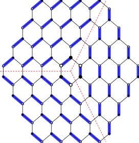
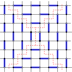
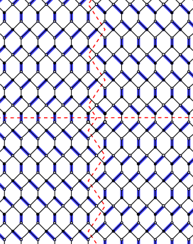
Figure 8. “Pyramids” for the square, hexagon and square-hexagon graphs. The matchings are intended to extend over the whole infinite graph. The dotted lines separate the domains tiled with different periodic matchings of extremal slope.

For each of the three graphs (square, hexagon, square-hexagon) consider the special matching $p\in\Omega$ (“$p$” for “pyramid” for reasons to become clear soon) of the whole $G$, defined through Fig. 8. Note that in all three cases $G$ is divided into a finite number of infinite domains, separated by dotted lines (three domains for the hexagon graph and four for the square and square-hexagon graph): each domain corresponds to a vertex in the Newton polygon $N$ of $G$ and it is tiled with the periodic matching corresponding to that vertex (cf. Fig. 1). The central face $f_{0}$ is assumed to contain the origin of ${\mathbb{R}}^{2}$ and we fix the height there to $0$. The large-scale height function ${\mathbb{R}}^{2}\ni x\mapsto H(x)$, obtained by rescaling the lattice spacing and the heights by $1/L\to 0$ while keeping $f_{0}$ at the origin of the plane can be described as follows. For each vertex $v$ of $N$, take the plane of the corresponding slope which contains the origin of ${\mathbb{R}}^{3}$, and let $s_{v}$ be the half-space below it. The intersection of all the $s_{v}$ with $v$ ranging over the vertices of $N$ is clearly a pyramid $\Pi$ with vertex at the origin of ${\mathbb{R}}^{3}$. The boundary of $\Pi$ gives the height function $H(\cdot)$. It is possible to prove (but we will not need this directly) that the discrete height function associated to matching $p$ is given by $h(f)=-D(f,f_{0})$, cf. Section 2.5.1. This observation could be used to build “pyramids” in a systematic way, for other graphs.

Remark 5.8.

For the hexagonal lattice, the pyramid $p$ just corresponds (in terms of stepped surfaces, cf. Fig. 2) to the surface of the corner of an infinite cube with vertex at the origin of ${\mathbb{R}}^{3}$.

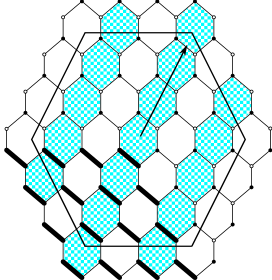
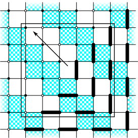
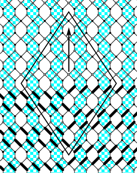
Figure 9. The sub-graph $W_{L}$ and the associated beads of configuration $p$. Threads are in light blue and white and beads are in solid black. Arrows mark the orientation of threads.

Next, we need to introduce a finite sub-graph $W_{L}\subset G$, with the face $f_{0}$ in the center. This is defined through Fig. 9: for the hexagonal lattice this is the portion of $G$ included in a $(2L+1)\times(2L+1)\times(2L+1)$ hexagon, for the square lattice it is a $(2L+1)\times(2L+1)$ square and for the square-hexagon lattice it is the portion of $G$ contained in a suitable lozenge (delimited by a full line in the picture) whose diagonals contain $2L+1$ hexagons. Note that the maximal configuration in $\Omega_{p,W_{L}}$ is just $p$: indeed, just observe that none of the beads in $W_{L}$ can be moved to a lower transverse edge in the same thread.

Proposition 5.9.

Consider the asynchronous fast dynamics on the finite graph $W_{L}$ defined above, with “pyramid” boundary condition $p$. Let $M^{max}_{t}$ (resp. $M^{eq}_{t}$) denote the state at time $t$ of the dynamics started from the maximal configuration, which is nothing but $p$ (resp. from the equilibrium uniform measure $\pi_{p,W_{L}}$) and let $\mathcal{F}_{t}$ be the sigma-algebra generated by $\{M^{max}_{s},M^{eq}_{s},s\leq t\}$. Remark that $M^{eq}_{t}$ is stationary. Let $V_{t}=\sum_{f\in W_{L}}[h_{M^{max}_{t}}(f)-h_{M^{eq}_{t}}(f)]$. Then, for every $t\;\geqslant\;t^{\prime}$

$$\mathbb{E}\bigl{[}V_{t}-V_{t^{\prime}}|\mathcal{F}_{t^{\prime}}\bigr{]}\;\geqslant\;-CL(t-t^{\prime})$$

for a certain constant $C$.

Proof.

The two evolutions can be coupled so that the one started from $p$ always dominates the stationary one. Therefore, it is sufficient to prove that, given two height functions $h^{-}\leq h^{+}$, the initial-time drift of their volume difference, see (4.4), is lower bounded by $-CL$. Let $\partial^{-}W_{L}$ denote the set of faces in $W_{L}$ at graph-distance at most $r$ from the exterior of $W_{L}$ and assume the following

Claim 5.10.

There exists some finite $r$ such that the initial-time volume drift is zero whenever $h^{+}$ and $h^{-}$ differ at a single face $f\in W_{L}\setminus\partial^{-}W_{L}$.

As in the proof of Proposition 4.10, take a sequence of configurations $h_{(0)},\dots,h_{(k)}$ such that $h_{(0)}=h^{+},h_{(k)}=h^{-}$ and $h_{(i)}$ is obtained by $h_{(i-1)}$ via a rotation that decreases the height at some face $f$. Along the sequence $\{h_{(i)}\}_{i}$, each face in $\partial^{-}W_{L}$ can be rotated at most a number $c(r)$ of times (since its height difference w.r.t. a face outside $W_{L}$ at distance $r$ can take at most $c(r)=2r+1$ values). Then write the volume difference between $h^{+}$ and $h^{-}$ as a telescopic sum of volume differences between $h_{(i)}$ and $h_{(i-1)}$: the terms corresponding to a rotation in $W_{L}\setminus\partial^{-}W_{L}$ give zero drift (cf. Claim 5.10) and those with rotation in $\partial^{-}W_{L}$ give a contribution lower bounded by $-1$ (cf. Remark 4.11). Then, one gets that the volume drift is lower bounded by $-c(r)$ times the number of faces in $\partial^{-}W_{L}$, which is of order $L$, and Proposition 5.9 follows. ∎

Proof of Claim 5.10.

In order to follow, the reader should have in mind the proof of Proposition 4.10: there we proved that the initial-time volume drift is zero except for “boundary effects”, and here we show that indeed the boundary effects are not there sufficiently far away from the boundary. As in the proof of Proposition 4.10, we consider for definiteness only the square-hexagon lattice, the other two cases being very similar. Note that there are $2L+1$ threads intersecting $W_{L}$ (we label them $\gamma_{i},i=-L,\dots,L$ from left to right) and that thread $\gamma_{i}$ contains $L+1-|i|$ beads in $W_{L}$ (we label them $b^{i}_{j},j=1,\dots,L+1-|i|$ from the lowest to the highest with respect to the orientation of the thread, see Fig. 10(a) for a schematic drawing). This geometric structure is essential for the proof of the Claim and, as the reader can check from Fig. 9, it is common to the “pyramids” of the three types of graphs. The effect of the boundary of $W_{L}$ is simply that the beads of thread $\gamma_{i}$ are constrained to stay strictly below some transverse edge $e^{+}_{i}\in\gamma_{i}$ and strictly above some transverse edge $e^{-}_{i}\in\gamma_{i}$ (such edges are surrounded by circles in Fig. 10(a)).

By symmetry, we assume that the face $f$ belongs to $\gamma_{i}$ for some $-L+r\leq i\leq 0$ (the case $-L\leq i<-L+r$ is excluded otherwise $f\in\partial^{-}W_{L}$) and assume for definiteness that $f$ is a hexagonal face (the argument is essentially identical when $f$ is a square). Then, $h^{+}$ is obtained from $h^{-}$ by moving a bead $b^{i}_{j}$ one “transverse edge” lower along thread $\gamma_{i}$ (with the notations of the proof of Proposition 4.10 (Case 1), $b=b^{i}_{j}$ moves from $e_{1}$ to $e_{2}$). We need to show that, if $f\in W_{L}\setminus\partial^{-}W_{L}$, when threads of the opposite parity than $i$ are updated while the threads with the same parity as $i$ are frozen, thread $\gamma_{i-1}$ contributes exactly $1/2$ to the change of volume (the same holds for $\gamma_{i+1}$).

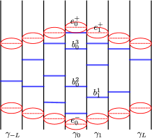
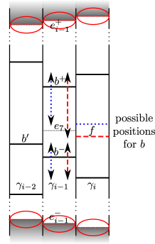
(a) (b) (c)

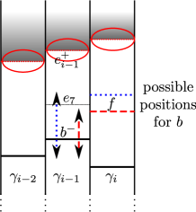
Figure 10. (a): A schematic view of the threads and beads in $W_{L}$ (here, $L=3$). (b): The case $1<j<L+1-|i|$. Here, $i=0$ and $j=3$. Boundary conditions only prevent beads from entering the gray region outside $W_{L}$, so they cannot prevent $b^{+}$ from moving down to $e_{7}$. (c): The case $j=L+1-|i|$. If $f\in\partial^{-}W_{L}$ then $e_{7}$ can be at $e^{+}_{i-1}$, in which case it is not an allowed bead position; otherwise, $e_{7}$ is in $W_{L}$ (since it is at distance of order $1$ from $f$) and $b^{-}$ can reach such position.

We distinguish two cases, represented respectively in Figures 10(b) and 10(c):

• $1<j<L+1-|i|$. Recall that from Section 4.2.4 that, according to the position of $b^{i-2}_{j-1}$ (which was called $b^{\prime}$ there), either $b^{i-1}_{j}$ (which was called $b^{+}$) has one more available transverse edge (called $e_{7}$) when the configuration before the update is $h^{+}$ rather than $h^{-}$, or otherwise $b^{i-1}_{j-1}$ (which was called $b^{-}$) has one more available transverse edge (again $e_{7}$) starting from $h^{-}$ rather than from $h^{+}$. Say that the former is the case. As discussed in Remark 4.11, the volume change due to thread $\gamma_{i-1}$ is $1/2$ unless the boundary conditions prevent $b^{+}$ from moving down to $e_{7}$, i.e. if $e_{7}$ is not higher than $e^{-}_{i-1}$: this however cannot be the case, since $e_{7}$ is clearly higher than $b^{-}=b^{i-1}_{j-1}$ which is itself higher than $e^{-}_{i-1}$ (here we use that $j-1\geq 1$, i.e. the bead $b^{i-1}_{j-1}$ is in $W_{L}$).

• $j=L+1-|i|$ (or $j=1$, by symmetry). The argument is slightly different since this time neither $b^{+}=b^{i-1}_{j}$ nor $b^{\prime}=b^{i-2}_{j-1}$ exist (since $j>L+1-|i-1|$), or equivalently we can imagine that $b^{+},b^{\prime}$ are higher than $e^{+}_{i-1},e^{+}_{i-2}$ respectively (i.e. they are outside $W_{L}$). Since the edge $e_{3}$ of Fig. 6 is at distance of order $1$ from $f$, we deduce that if $f$ is at distance larger than some finite $r$ from the boundary of $W_{L}$ then $b^{\prime}$ is above $e_{3}$. In this case, from Section 4.2.4, we get that $b^{-}$ has one more available position (transverse edge $e_{7}$) when the update of $\gamma_{i-1}$ is performed starting from configuration $h^{-}$ rather than $h^{+}$. It is clear from Fig. 9 and 6 that, if $f$ is at distance at least $r$, with $r$ sufficiently large, from the boundary of $W_{L}$, the edge $e_{7}$ is lower than $e^{+}_{i-1}$, so there is no obstruction for $b^{-}$ to actually reach it.

∎

5.2.2. Lower bound on mixing time

Figure 11. An illustration of the proof of the lower bound. The pyramid and, above it, the maximal configuration with planar boundary condition $m$. The top of the pyramid is $O(L)$ above the typical “almost-planar” equilibrium configuration (wiggled line). After a time $\epsilon L^{2}$, the pyramid has only lost a volume $\epsilon L^{3}$, so its top is still well above the “almost-planar” surface. By stochastic domination, the same holds for the maximal evolution with boundary condition $m$.

Recall Definition 2.2: the finite graph $G^{\prime}$ we are interested in is the portion of $G$ enclosed in $LU$, where $U$ is a smooth bounded domain of ${\mathbb{R}}^{2}$, which without loss of generality we can assume to include the origin in its interior (so that $f_{0}$ is at distance of order $L$ from the boundary of $G^{\prime}$). Now consider the finite graph $W_{\ell}\subset G$ defined in Section 5.2.1, and choose $\ell$ to be the minimal integer such that $W_{\ell}\supset G^{\prime}$ (it is clear that $\ell=O(L)$).

Consider first the evolution in $W_{\ell}$ with boundary condition $p$ (and started from the maximal configuration $p$): by Proposition 5.9 and Markov’s inequality we have that at time $T_{0}=\epsilon L^{2}$,

$$\mathbb{P}(h_{T_{0}}(f_{0})\leq-\epsilon^{1/4}L)=O(\epsilon^{1/4})$$ (5.5)

(indeed observe that, if $h(f_{0})<-\epsilon^{1/4}L$ then the eroded volume is at least $const\times(\epsilon^{1/4}L)^{3}\simeq LT_{0}\epsilon^{-1/4}$ while the average eroded volume is of order $LT_{0}$).

Now recall that the boundary condition $m$ we are interested in is almost-planar of slope $(s,t)$: up to an irrelevant global change of the heights by an additive constant, we can assume that its height function $h_{m}(\cdot)$ is within $O(1)$ from a plane of slope $(s,t)$ and containing the point $(0,0,-2\epsilon^{1/4}L)$. If $h_{p}(\cdot)$ is the height function associated to the “pyramid” matching $p$ and if $\epsilon$ is sufficiently small, $h_{m}(f)\geq h_{p}(f)$ for every $f$ along the boundary of $G^{\prime}$ (the height difference is actually of order $L$). To see this, just recall that the slope of the height function associated to $p$ is negative and maximal (in absolute value) along any straight line starting from $f_{0}$, while the slope $(s,t)$ is in the interior of the Newton polygon, so it is not an extremal slope (see Figure 11). Note that $\epsilon$ has to be taken very small if the slope $(s,t)$ is very close to $\partial N$.

We have then that, by monotonicity, the evolution in $G^{\prime}$, with boundary condition $m$ and started from the maximal configuration, is stochastically higher than the restriction to $G^{\prime}$ of the evolution in $W_{\ell}$ with boundary condition $p$. As a consequence, for the former dynamics we have that (5.5) still holds. Thanks to Theorem 2.9, at equilibrium (with almost-planar boundary condition $m$) the typical equilibrium height at $f_{0}$ is around $-2L\epsilon^{1/4}$ and the probability that it is higher than $-L\epsilon^{1/4}$ tends to zero with $L$. This suffices to conclude that at time $T_{0}$ the variation distance from equilibrium is still close to $1$. ∎

Appendix A Gaussian behavior of fluctuations

In this section we prove Theorem 2.8. The proof is quite independent of the rest of the paper. The main tools are the results from [12] that were stated in Section 2.2. The proof is very similar to that of [11, Section 7] but the setting here is more general and we give a more explicit control of the “error terms”.

From the definition of height function, we know that $h(f)-h(g)$ is determined by the dimers crossed by a path from $f$ to $g$. In particular, for the square, hexagon and square-hexagon graphs, assume that $f$ and $g$ are on the same thread (cf. Section 4.1): then, $h(f)-h(g)$ is determined just by the number $N_{f,g}$ of such dimers. Label $e_{1},\dots,e_{k}$ the transverse edges between $f$ and $g$: it is easy to realize, using Theorem 2.4, that the set of occupied edges among the $e_{i}$ forms a determinantal point process: in other words, the probability $\mu_{s,t}(e_{i_{1}}\in M,\dots,e_{i_{m}}\in M)$ can be written as $\det(A(i_{a},i_{b})_{1\leq a,b\leq m})$ for a certain $k\times k$ matrix $A$ directly related to $K^{-1}_{s,t}$. Now, it turns out [8] that for the hexagonal lattice such matrix is Hermitian. In this case, a well-known theorem by Costin and Lebowitz (cf. for instance [22]) implies that $N_{f,g}$ is distributed like the sum of independent Bernoulli random variables, whose parameters are the eigenvalues of $A$. In particular, if the variance of $N_{f,g}$ diverges as $k\to\infty$, the variable $[N_{f,g}-\mu_{s,t}(N_{f,g})]/\sqrt{{\operatorname{Var}}(N_{f,g})}$ tends to $\mathcal{N}(0,1)$. Unfortunately, for the square and square-hexagon graph the matrix $A$ is not Hermitian and has complex eigenvalues, the Costin-Lebowitz theorem does not apply and the asymptotic moments have to be computed otherwise.

A.1. Choice of paths

Fix an integer $k$. We are interested in the behavior of

$$\mu_{s,t}\left[M(f,f^{\prime})^{k}\right]=\mu_{s,t}\left(\Bigl{[}\bigl{(}h(f)-\mu_{s,t}(h(f))\bigr{)}-\bigl{(}h(f^{\prime})-\mu_{s,t}(h(f^{\prime}))\bigr{)}\Bigr{]}^{k}\right)$$ (A.1)

when the distance between $f$ and $f^{\prime}$ goes to infinity. Remark that for any path $C$ on $G^{*}$ from $f$ to $f^{\prime}$ that only crosses edges in the positive direction, $h(f^{\prime})-h(f)$ is exactly the difference between the number of dimers crossed by the random matching minus those crossed by the reference matching, so $M(f,f^{\prime})=\sum_{e}[1_{e\in M}-\mu_{s,t}(e\in M)]$ with the sum over all edges crossed by $C$. We will compute moments of higher order by taking $k$ such paths $C_{1},\ldots,C_{k}$ :

$$\mu_{s,t}\left[M(f,f^{\prime})^{k}\right]=\mu_{s,t}\Bigl{[}\sum_{e_{1}\in C_{1}}\left(\delta_{e_{1}}-\mu_{s,t}(\delta_{e_{1}})\right)\ldots\sum_{e_{k}\in C_{k}}\left(\delta_{e_{k}}-\mu_{s,t}(\delta_{e_{k}})\right)\Bigr{]}$$ (A.2)

where we write $\delta_{e}$ for $1_{e\in M}$.

Figure 12. The paths $C_{1},\dots,C_{k}$ (here $k=5$) along which is computed the height, displayed at large scale so that they look like continuous curves. They are macroscopically away from each other except near $f$ and $f^{\prime}$ where they are periodic (so that on large scale they look linear).

In principle we can choose the paths $C_{1}\ldots,C_{k}$ freely as long as they only cross edges in the positive direction. In practice, for reasons that will be clear later we will adopt the following construction, illustrated in Fig. 12. Fix $\eta,\eta^{\prime}>0$. Inside balls of radius $\eta L$ around $f$ and $f^{\prime}$, the $C_{i}$ are portions of length $\eta L$ of infinite periodic paths (cf. Definition 2.1) and have mutually different asymptotic directions. Outside of these balls the paths stay at distance at least $\eta^{\prime}L$ of each other and their length is of order $L$. Furthermore $\eta,\eta^{\prime}$ and the infinite periodic paths depend on $k$ but not on $L$.

A.2. Exact simplifications

Fix $k$ edges $e_{1}=({\rm w}_{1},{\rm b}_{1})\in C_{1},\ldots,e_{k}=({\rm w}_{k},{\rm b}_{k})\in C_{k}$, and consider the corresponding term (written $\Pi(e_{1},\ldots,e_{k})$) of the sum (A.2).

We write $\delta_{i}$ for $\delta_{e_{i}}$, $K^{-1}_{i,j}$ for $K_{s,t}^{-1}({\rm b}_{i},{\rm w}_{j})$ and $K_{ij}$ for $K_{s,t}({\rm w}_{i},{\rm b}_{j})$. We also write $S_{k}$ the set of permutations of $\{1,\ldots,k\}$, $\tilde{S}_{k}$ the set of permutations without fixed points and $\tilde{S}_{k}^{2}$ those of order $2$. Given $\sigma\in S_{k}$, we denote $\epsilon(\sigma)$ it signature.

First we express each term $\Pi(e_{1},\ldots,e_{k})$ of the sum (A.2) as a sum over permutations with no fixed points.

Lemma A.1.

Given edges $e_{1},\ldots,e_{k}$ as above, we have

$$\Pi(e_{1},\ldots,e_{k})\equiv\mu_{s,t}\bigl{[}\prod_{n=1}^{k}\bigl{(}\delta_{n}-\mu_{s,t}(\delta_{n})\bigr{)}\bigr{]}=\prod_{n=1}^{k}K_{nn}\sum_{\sigma\in\tilde{S}_{k}}\epsilon(\sigma)\prod_{n=1}^{k}K^{-1}_{n\sigma(n)}.$$ (A.3)

This is exactly like [9, Lemma 21].

Now we replace $K^{-1}_{n\sigma(n)}$ by its asymptotic expression from Theorem 2.6. To lighten notations we use the following conventions. Recall that $e_{i}=({\rm w}_{i},{\rm b}_{i})$ and write (in a unique way) ${\rm b}_{i}=\hat{\rm b}_{i}+(x_{i},y_{i}),{\rm w}_{i}=\hat{\rm w}_{i}+(x^{\prime}_{i},y^{\prime}_{i})$ with $\hat{\rm b}_{i},\hat{\rm w}_{i}$ in the fundamental domain $G_{1}$ and $(x_{i},y_{i})\in{\mathbb{Z}}^{2},(x^{\prime}_{i},y^{\prime}_{i})\in{\mathbb{Z}}^{2}$. Note that $(x_{i}-x^{\prime}_{i},y_{i}-y^{\prime}_{i})$ is a vector of order $1$. Then let $U_{i}:=U_{s,t}(\hat{\rm b}_{i})$, $V_{j}:=V_{s,t}(\hat{\rm w}_{j})$ and $\phi_{i}:=\phi(x_{i},y_{i})$, $x_{ij}=x^{\prime}_{i}-x_{j}$ and $y_{ij}=y^{\prime}_{i}-y_{j}$. We then get

$$\Pi(e_{1},\dots,e_{k})/\Bigl{(}\prod_{n=1}^{k}K_{nn}\Bigr{)}=\sum_{\sigma\in\tilde{S}_{k}}\epsilon(\sigma)\prod_{n=1}^{k}\left(i\frac{U_{n}V_{\sigma(n)}w_{0}^{x_{n\sigma(n)}}z_{0}^{y_{n\sigma(n)}}}{2\pi(\phi_{n}-\phi_{\sigma(n)})}+\text{complex conjugate}\right.\\ \left.+O\Big{(}\frac{1}{x_{n\sigma(n)}^{2}+y_{n\sigma(n)}^{2}}\Big{)}\right)\equiv\sum_{\sigma\in\tilde{S}_{k}}\epsilon(\sigma)\prod_{n=1}^{k}(A_{n,\sigma(n)}+A^{*}_{n,\sigma(n)}+R_{n,\sigma(n)}).$$ (A.4)

We then expand the product over $n$ and we call “dominant terms” those such that no $R$ factors appear and, in addition, such that within each cycle of $\sigma$ either only $A$ terms or only $A^{*}$ terms appear. All other terms of the expansion are called “error terms”. We first show that in the dominant terms we can assume that all cycles of the permutation $\sigma$ are of order two. This comes from the following result:

Lemma A.2.

If $\tilde{S}^{c}_{\ell}$ denotes the set of cyclic permutations of $\{1,\dots,\ell\}$, then

$$\sum_{\sigma\in\tilde{S}^{c}_{\ell}}\epsilon(\sigma)\prod_{n=1}^{\ell}A_{n\sigma(n)}=\sum_{\sigma\in\tilde{S}^{c}_{\ell}}\epsilon(\sigma)\prod_{n=1}^{\ell}\frac{i}{2\pi}\frac{U_{n}V_{\sigma(n)}w_{0}^{x_{n\sigma(n)}}z_{0}^{y_{n\sigma(n)}}}{\phi_{n}-\phi_{\sigma(n)}}=0\left(=\sum_{\sigma\in\tilde{S}^{c}_{\ell}}\epsilon(\sigma)\prod_{n=1}^{\ell}A^{*}_{n\sigma(n)}\right)$$ (A.5)

if $\ell>2$.

Proof.

Recall that $\epsilon(\sigma)$ is constant for cyclic permutations, thus it is enough to show that

$$\sum_{\sigma\in\tilde{S}^{c}_{\ell}}\prod_{n}\frac{U_{n}V_{\sigma(n)}w_{0}^{x_{n\sigma(n)}}z_{0}^{y_{n\sigma(n)}}}{\phi_{n}-\phi_{\sigma(n)}}=\prod_{n}\left(U_{n}V_{n}\right)w_{0}^{\sum_{i}(x^{\prime}_{i}-x_{i})}z_{0}^{\sum_{i}(y^{\prime}_{i}-y_{i})}\sum_{\sigma\in\tilde{S}_{\ell}^{c}}\prod_{n}\frac{1}{\phi_{n}-\phi_{\sigma(n)}}=0$$ (A.6)

as soon as $\ell>2$. The second equality is purely algebraic and is given in [11, Lemma 7.3]. ∎

Decompose a permutation $\sigma$ into cycles and remark that in equation (A.3) and (A.4), the sum over permutations with a given cycle structure can be factorized as a product over cycles. Then, Lemma A.2 implies that the dominant terms in

$$\sum_{\sigma\in\tilde{S}_{k}\setminus\tilde{S}^{2}_{k}}\epsilon(\sigma)\prod_{n=1}^{k}(A_{n,\sigma(n)}+A^{*}_{n,\sigma(n)}+R_{n,\sigma(n)})$$

exactly cancel each other so only “error terms” are left (recall that $\tilde{S}^{2}_{k}$ is the set of permutations without fixed points, and with only cycles of order $2$). Altogether, we have proven (cf. (A.4))

$$\mu_{s,t}(M(f,f^{\prime})^{k})=\sum_{e_{1}\in C_{1}}\cdots\sum_{e_{k}\in C_{k}}\sum_{\sigma\in\tilde{S}_{k}^{2}}\epsilon(\sigma)\left(\prod_{n=1}^{k}K^{-1}_{n\sigma(n)}\right)\left(\prod_{n=1}^{k}K_{nn}\right)+\text{error terms}.$$ (A.7)

In particular, if $k$ is odd then there are only “error terms” because $\tilde{S}^{2}_{k}$ is empty, while, using equation (A.3) separately for all pairs,

$$\mu_{s,t}(M(f,f^{\prime})^{2k}) =\sum_{\sigma\in\tilde{S}_{2k}^{2}}\mu_{s,t}[M(f,f^{\prime})^{2}]^{k}+\text{error terms}$$ (A.8)

$$=g_{2k}\left[\operatorname{Var}_{\mu_{s,t}}(h(f)-h(f^{\prime}))\right]^{k}+\text{error terms}$$ (A.9)

where $g_{2k}=(2k)!/(2^{k}k!)$ is the Gaussian moment of order $2k$. We will prove in the following section that the error terms are negligible, i.e. give a contribution to $\mu_{s,t}(M(f,f^{\prime})^{k})$ that is much smaller than $[\operatorname{Var}_{\mu_{s,t}}(h(f)-h(f^{\prime}))]^{k/2}$.

A.3. Controlling the “error terms”

Recall that there are two kinds of “error terms” in the expression (A.7) for the $k$-th moment of the height fluctuation: those which contain both $A$ and $A^{*}$ factors within the same cycle of $\sigma$ but but no $R$ factor (recall (A.4)), and those which contain $R$ factors. The former will be shown to be “small” because they oscillate and give a negligible contribution when summed over $e_{1},\dots,e_{k}$, while the latter are small because their denominator contains at least one factor $|\phi_{j}-\phi_{\sigma(j)}|$ more than in the dominant terms. For simplicity purpose we assume in the following that $\sigma$ contains only a single cycle. The general case is essentially the same since an error term can be factorized as a product over the cycles of $\sigma$.

We will need the following elementary estimates:

Lemma A.3.

Define

$$F_{k}(L)=\sum_{d_{1},\dots,d_{k}\leq L}\frac{1}{(d_{1}+d_{2})\dots(d_{k}+d_{1})},\quad\tilde{F}_{k}(L)=\sum_{d_{1},\dots,d_{k}\leq L}\frac{1}{(d_{1}+d_{2})\dots(d_{k-1}+d_{k})}.$$ (A.10)

One has $\tilde{F}_{k}(L)\leq LF_{k-1}(L)$ and $F_{k}(L)=O((\log L)^{\lfloor k/2\rfloor}).$

Proof.

To get $\tilde{F}_{k}(L)\leq LF_{k-1}(L)$, writing $F_{k-1}(L)$ either as a sum over $d_{1},\dots,d_{k-1}$ or over $d_{2},\dots,d_{k}$ it is not difficult to see that

$$2LF_{k-1}(L)-2\tilde{F}_{k}(L)=\sum_{d_{1},\dots,d_{k}}\frac{1}{(d_{1}+d_{2})\dots(d_{k-2}+d_{k-1})}\,\frac{(d_{1}-d_{k})^{2}}{(d_{1}+d_{k-1})(d_{2}+d_{k})(d_{k-1}+d_{k})}\geq 0$$

(use the fact that the denominator is symmetric under the exchange of $d_{1}$ with $d_{k}$). As for $F_{k}(L)=O((\log L)^{\lfloor k/2\rfloor})$, this is an easy computation if $k=2$. By induction on $k$, the proof is concluded if we show that $F_{k}(2L)-F_{k}(L)=O(kF_{k-2}(L))$ for $k\geq 4$ and $F_{k}(2L)-F_{k}(L)=O(1)$ for $k=3$. To see this, one notes that the dominant contribution to $F_{k}(2L)-F_{k}(L)$ comes from the terms where one of the variables is in $[L,2L]$ while all the others are smaller than $L$: altogether, this gives

$$\sum_{i=1}^{k}\sum_{d_{1},\ldots d_{k}\;\leqslant\;L}\frac{1}{(d_{1}+d_{2})\ldots(d_{i-1}+(L+d_{i}))((L+d_{i})+d_{i+1})\ldots(d_{k}+d_{1})} \;\leqslant\;kL\tfrac{1}{L^{2}}\tilde{F}_{k-1}(L).$$

For $k>3$ use $\tilde{F}_{k-1}(L)\leq LF_{k-2}(L)$ and for $k=3$ note that $\tilde{F}_{2}(L)=O(L)$. ∎

The first remark about the computation of $\mu_{s,t}(M(f,f^{\prime})^{k})$ is that we can restrict ourselves to the cases where either all edges $e_{i}$ are in the ball $B_{f}(\eta L)$ of radius $\eta L$ around either $f$ or in the analogous ball around $f^{\prime}$. Indeed, call $d_{i}$ the distance of $e_{i}$ from $f$ and observe that, since the map $\phi$ is non-degenerate and the paths $C_{i}$ are almost linear in $B_{f}(\eta L)$, one can bound $|\phi_{i}-\phi_{j}|$, from above and below, by a constant times $(d_{i}+d_{j})$. Then the sum of (A.4) with, for example, $e_{1},\dots,e_{k-1}$ in $B_{f}(\eta L)$ and $e_{k}$ out of $B_{f}(\eta L)$ is of order $(1/L)\tilde{F}_{k-1}(\eta L)\leq F_{k-2}(\eta L)=O((\log L)^{\lfloor k/2\rfloor-1})\ll[\operatorname{Var}_{\mu_{s,t}}(h(f)-h(f^{\prime}))]^{k/2}$. Terms with more than one $e_{i}$ outside of $B_{f}(\eta L)$ are even smaller. To fix ideas, we will assume that all $e_{i}$ are in $B_{f}(\eta L)$.

Consider now an “error term” containing a factor $R$ (if it contains more than one, the argument is similar). Summing over $e_{i}$, this gives a contribution of order

$$\sum_{d_{1},\dots,d_{k}\;\leqslant\;\eta L}\frac{1}{(d_{1}+d_{2})\ldots(d_{k}+d_{1})}\frac{1}{d_{1}+d_{2}}\;\leqslant\;\sum_{d_{2},\ldots,d_{k}}\frac{1}{(d_{2}+d_{3})\ldots(d_{k-1}+d_{k})}\sum_{u=d_{2}}^{\infty}\frac{1}{d_{k}u^{2}}$$ (A.11)

$$\;\leqslant\;const\times\sum_{d_{2},\ldots,d_{k}}\frac{1}{(d_{2}+d_{3})\ldots(d_{k}+d_{2})}\frac{d_{2}+d_{k}}{d_{2}d_{k}}=O(F_{k-1}(\eta L))\ll[\operatorname{Var}_{\mu_{s,t}}(h(f)-h(f^{\prime}))]^{k/2}.$$

We still have to deal with the error terms including no $R$ factors but both $A$ and $A^{*}$ within the same cycle of $\sigma$. Recall that for simplicity of exposition that $\sigma$ is assumed to have a single cycle. Omitting the product of the factors $\pm i/(2\pi)$, these terms are of the form

$$\sum_{e_{1},\dots,e_{k}}e^{i[r(x_{1},\ldots,x_{k})+s(y_{1},\ldots,y_{k})]}C(e_{1},\ldots,e_{k})\prod_{i\in J}\frac{1}{\phi_{i}-\phi_{\sigma(i)}}\prod_{i\in J^{c}}\frac{1}{{\phi^{*}}_{i}-{\phi^{*}}_{\sigma(i)}}$$ (A.12)

where $e_{j}$ runs over the edges crossed by path $C_{j}$ and:

• $J$ (resp. $J^{c}$) is the set of indices $n\in\{1,\dots,k\}$ for which we take $A_{n\sigma(n)}$ (resp. $A^{*}_{n\sigma(n)}$) in the expansion of the product (A.4). Note that both $J$ and $J^{c}$ are non-empty, proper subsets of $\{1,\dots,k\}$;

• $C(e_{1},\dots,e_{k})$ depends only on the types of the $k$ edges (two edges being of the same type if they are related by a translation of ${\mathbb{Z}}^{2}$):

  $$C(e_{1},\dots,e_{k})=\prod_{i\in J}\left(U_{i}V_{\sigma(i)}w_{0}^{(x^{\prime}_{i}-x_{i})}z_{0}^{(y^{\prime}_{i}-y_{i})}\right)\prod_{i\in J^{c}}\left(U^{*}_{i}V^{*}_{\sigma(i)}w_{0}^{-(x^{\prime}_{i}-x_{i})}z_{0}^{-(y^{\prime}_{i}-y_{i})}\right);$$

• $r,s$ are linear functions: if $J^{\prime}=\{i\in J:\sigma^{-1}(i)\in J^{c}\}$ and $J^{\prime\prime}=\{i\in J^{c}:\sigma^{-1}(i)\in J\}$ (remark that $|J^{\prime}|=|J^{\prime\prime}|\neq 0$ otherwise $\sigma$ would have more than one cycle) and writing $w_{0}=\exp(i\theta_{w}),z_{0}=\exp(i\theta_{z})$,

  $$r(x_{1},\dots,x_{k})+s(y_{1},\dots,y_{k})=2\theta_{w}(\sum_{a\in J^{\prime}}x_{a}-\sum_{a\in J^{\prime\prime}}x_{a})+2\theta_{z}(\sum_{a\in J^{\prime}}y_{a}-\sum_{a\in J^{\prime\prime}}y_{a}).$$

Splitting the sum $\sum_{e_{1},\dots,e_{k}}$ over the different types of edges, we can assume without loss of generality that all edges in each path are of the same type (so that $C(e_{1},\dots,e_{k})$ becomes a constant; edge types can be different in different paths) and that edges in the path $j$ are obtained one from the other via translations by an integer multiple of some $v^{(j)}=(v^{(j)}_{1},v^{(j)}_{2})\in{\mathbb{Z}}^{2}$. The edges in the $j$-th path will be labeled by an integer $d_{j}$, which runs from $1$ to $M_{j}=O(\eta L)$ and $r(x_{1},\ldots,x_{k})+s(y_{1},\ldots,y_{k})$ becomes is a linear function of $d_{1},\dots,d_{k}$.

Assume without loss of generality that $1\in J^{\prime}$. From the discussion above we obtain that

$$(r+s)(d_{1},\dots,d_{k})=(r+s)(0,d_{2},\dots,d_{k})+2(\theta_{w}v^{(1)}_{1}+\theta_{z}v^{(1)}_{2})d_{1}.$$

Despite the fact that $w_{0},z_{0}$ are unit complex numbers with phase different from $0,\pi$ it could happen that $\Theta:=2(\theta_{w}v^{(1)}_{1}+\theta_{z}v^{(1)}_{2})$ is a multiple of $2\pi$, so that $\exp(i(r+s))$ is independent of $d_{1}$: this can however be avoided if the asymptotic directions and the period of path $C_{1}$ in $B_{f}(\eta L)$ are chosen suitably (we skip tedious details on this point).

We separate the sum over $e_{1}$ from the others and we make a summation by parts to get:

$$const\times\sum_{e_{2},\ldots,e_{k}}\frac{e^{i(r+s)|_{d_{1}=0}}}{(\tilde{\phi}_{2}-\tilde{\phi}_{3})\ldots(\tilde{\phi}_{k-1}-\tilde{\phi}_{k})}$$ (A.13)

$$\times\left[\sum_{d_{1}}\Bigl{(}\sum_{d\;\leqslant\;d_{1}}e^{i\Theta d}\Bigr{)}\frac{\Delta\tilde{\phi}_{1}(\tilde{\phi}_{k}+\tilde{\phi}_{2}-2\tilde{\phi}_{1}(d_{1})-\Delta\tilde{\phi}_{1})}{\bigl{(}\tilde{\phi}_{1}(d_{1})-\tilde{\phi}_{2}\bigr{)}\bigl{(}\tilde{\phi}_{k}-\tilde{\phi}_{1}(d_{1})\bigr{)}\bigl{(}\tilde{\phi}_{1}(d_{1}+1)-\tilde{\phi}_{2}\bigr{)}\bigl{(}\tilde{\phi}_{k}-\tilde{\phi}_{1}(d_{1}+1)\bigr{)}}+O\left(\frac{1}{d_{2}d_{k}}\right)\right]$$

where the $O(...)$ comes from boundary terms in the summation by parts (note that $\sum_{d\;\leqslant\;d_{1}}e^{i\Theta d}$ is bounded since $\Theta\neq 0$(mod $2\pi)$), $\Delta\tilde{\phi}_{1}=\tilde{\phi}_{1}(d_{1}+1)-\tilde{\phi}_{1}(d_{1})$ is constant by linearity of $\phi$ and for simplicity of notation $\tilde{\phi}_{i}$ can denote either $\phi_{i}$ or its complex conjugate. We can thus bound $\lvert\phi_{i}-\phi_{j}\rvert$ by $d_{i}+d_{j}$ as before and (up to a constant factor) the absolute value of (A.13) by

$$\sum_{d_{2},\ldots,d_{k}}\frac{1}{(d_{2}+d_{3})\ldots(d_{k-1}+d_{k})}\Bigl{(}\sum_{d_{1}}\frac{2d_{1}+d_{2}+d_{k}}{(d_{1}+d_{2})^{2}(d_{1}+d_{k})^{2}}+O\Bigr{(}\frac{1}{d_{2}d_{k}}\Bigr{)}\Bigr{)}$$ (A.14)

$$=\sum_{d_{2},\ldots,d_{k}}\frac{1}{(d_{2}+d_{3})\ldots(d_{k-1}+d_{k})(d_{2}+d_{k})}\Bigl{(}\sum_{d_{1}}\frac{(2d_{1}+d_{2}+d_{k})(d_{2}+d_{k})}{(d_{1}+d_{2})^{2}(d_{1}+d_{k})^{2}}+O\left(\frac{d_{2}+d_{k}}{d_{2}d_{k}}\right)\Bigr{)}$$ (A.15)

$$=O\bigl{(}F_{k-1}(\eta L)\bigr{)}\ll[\operatorname{Var}_{\mu_{s,t}}(h(f)-h(f^{\prime}))]^{k/2}$$ (A.16)

because the parenthesis in the second line is clearly bounded.

References

- [1] R. Brandenberger, C. E. Wayne, Decay of correlations in surface models, J. Statist. Phys. 27 (1982), 425–440.
- [2] J. Bricmont, A. El Mellouki, and J. Fröhhlich, Random surfaces in statistical mechanics: roughening, rounding, o wetting…, J. Statist. Phys. 29 (1982), 193–203.
- [3] P. Caputo, E. Lubetzky, F. Martinelli, A. Sly, F. L. Toninelli, Dynamics of 2+1 dimensional SOS surfaces above a wall: slow mixing induced by entropic repulsion, to appear on Ann. Probab., arXiv:1205.6884
- [4] P. Caputo, F. Martinelli, F. Simenhaus, F. L. Toninelli, “Zero” temperature stochastic 3D Ising model and dimer covering fluctuations: a first step towards interface mean curvature motion, Comm. Pure Appl. Math. 64 (2011), 778–831.
- [5] P. Caputo, F. Martinelli, F. L. Toninelli, Mixing times of monotone surfaces and SOS interfaces: a mean curvature approach, Comm. Math. Phys. 311 (2012), 157–189.
- [6] J. C. Fournier, Pavage des figures planes sans trous par des dominos: Fondement graphique de l’algorithme de Thurston, parallélisation, unicité et décomposition, Theoretical Computer Science, 159 (1996), 105-128.
- [7] P. W. Kasteleyn, The statistics of dimers on a lattice, I. The number of dimer arrangements on a quadratic lattice, Physica 27 (1961), 1209–1225.
- [8] R. Kenyon, Lectures on dimers, Statistical mechanics, 191–230, IAS/Park City Math. Ser., 16, Amer. Math. Soc., Providence, RI, 2009.
- [9] R. Kenyon, Conformal invariance of domino tiling, Ann. Probab. 28 (2000), 759-795.
- [10] R. Kenyon, Dominos and the Gaussian free field, Ann. Prob. 29, no. 3 (2001), 1128–1137.
- [11] R. Kenyon, Height fluctuation in the honeycomb dimer model, Comm. Math. Phys. 281 (2007), 675-709.
- [12] R. Kenyon, A. Okounkov, S. Sheffield, Dimers and amoebae, Annals of Mathematics, 163 (2006), 1019-1056.
- [13] R. Kenyon, J. G. Propp and D. B. Wilson, Trees and matchings, Elec. J. Comb. 7 (2000), RP25.
- [14] R. Kenyon and S. Sheffield, Dimer, tilings and trees, J. Comb. Theory B 92 (2004), 295–317
- [15] M. Mucha, P. Sankowski, Maximum matchings in planar graph via gaussian elimination, Algorithmica 45 (2006), 3–20
- [16] D. Levin, Y. Peres, E. Wilmer, Markov Chains and mixing times, Am. Math. Soc., Providence, RI, (2009).
- [17] M. Luby, D.Randall, A. Sinclair, Markov chain algorithms for planar lattice structures, SIAM Journal on Computing, 31 (2001), 167-192
- [18] Y. Peres, P. Winkler, Can extra update delay mixing?, Comm. Math. Phys. 323 (2013), 1007–1016.
- [19] L. Petrov, Asymptotics of Uniformly Random Lozenge Tilings of Polygons. Gaussian Free Field, arXiv:1206.5123.
- [20] D. Randall, P. Tetali, Analyzing Glauber Dynamics by Comparison of Markov Chains, J. Math. Phys. 41 (2000), no. 3, 1598–1615.
- [21] S. Sheffield, Random surfaces, Societé mathématique de France, Asterisque 305 (2005).
- [22] A. Soshnikov, Determinantal random point fields, Russ. Math. Surv. 55 (2000), 923–975.
- [23] H. Spohn, Interface motion in models with stochastic dynamics, J. Stat. Phys. 71 (1993), 1081–1132.
- [24] H. N. V. Temperley, Statistical mechanics and the partition of numbers. II. The form of crystal surfaces, Proc. Cambridge Philos. Soc. 48 (1952), 683–697.
- [25] H. N. V. Temperley and M. E. Fisher, Dimer problem in statistical mechanics–an exact result, Phil. Mag. 6 (1961), 1061–1063.
- [26] D. B. Wilson, Determinant algorithms for random planar structures, Proc. Eighth Annual ACM-SIAM Symposium on Discrete Algorithms (1997), 258–267.
- [27] D. B. Wilson, Generating random spanning trees more quickly than the cover time, Proc. of the 28th annual ACM symposium on Theory of computing (STOC ’96), 296-303.
- [28] D. B. Wilson, Mixing times of lozenge tiling and card shuffling Markov chains, Ann. Appl. Probab. 14 (2004), 274–325.