Quantization of almost-circular orbits in the Fokker action formalism. Regge trajectories.

Abstract

A relativistic quark model of mesons formulated within the formalism of Fokker-type action integrals is proposed, in which an interquark interaction is mediated by scalar-vector superposition of higher derivative fields. In the non-relativistic limit the model describes a two-particle system with the linear potential. In order to analyze the model in the essentially relativistic domain the perturbed circular orbit approximation and certain principle of selection of physically meaningful solutions are applied which permit one to perform the canonical quantization of the model. It is shown that the model reproduces well specific features of the light meson spectroscopy.

I Introduction

It is known that spectra of heavy mesons (contaning c and b quarks) are described well by means of potential models with the non-relativistic Cornell potential $u(r)=u_{0}-\alpha/r+ar$ and various quasi-relativistic corrections of scalar-vector type Eich75 ; LSG91 ; H-L92 ; H-M02 . The potential is QCD-motivated: its Coulomb part is a non-relativistic limit of the one-gluon exchange interaction while the linear part comes from the Wilson loop. The latter is also related to a string conception of hadrons Nie77 ; J-N79 ; Sim94 . Constants $u_{0}$, $\alpha$ and $a$ vary from one model to another. In particular, the string tension parameter $a$ is frequently used as an adjustable parameter from the range $a=0.15\div 0.3$ GeV² Eich75 ; LSG91 ; H-L92 ; H-M02 although the most conventional value $a=0.18\div 0.2$ GeV² is substantiated by QCD simulations on the lattice B-S09 .

Mass spectra of light mesons (consisting of u, d and s quarks) possess characteristic features which can be summarized roughly in the following idealized picture Sim94 ; B-P91 ; Duv06 ; Duv08 :

1. Meson states are clustered in the family of straight lines in the ($M^{2},j$)–plane known as Regge trajectories.

2. Regge trajectories are parallel; slope parameter $\sigma$ is an universal quantity, $\sigma=1.15\div 1.2\,{\rm GeV}^{2}$.

3. As states of quark-antiquark system mesons can be classified non-relativistically, by $\ell$ and $n_{r}$ (the orbital and radial quantum numbers) as well as by $s$ and $j$ (the total spin and angular momentum).

4. Spectrum is $\ell$$s$-degenerated, i.e., masses are distinguished by $\ell$ (not by $j$ or $s$) and $n_{r}$.

5. States of different $\ell$ and $n_{r}$ possess an accidental degeneracy which causes a tower structure of the spectrum.

Items 1–4 imply that in the ($M^{2},\ell$)–plane meson states form into strait lines too: the principal ($n_{r}=0$) Regge trajectory built up of the set of degenerated singlet ($s=0$) and triplet ($s=1$) states, and the family of daughter trajectories ($n_{r}=1,2,\dots$). Hence energy levels of q-q̄ system can be described by a formula:

$$M^{2}\approx\sigma(\ell+\varkappa n_{r}+\zeta),$$ (1)

where the intercept constant $\zeta$ depends on a flavor content of mesons ($\zeta\approx 1/2$ for ($\pi$-$\rho$)–family of mesons; it grows together with quark masses). Finally, the accident degeneracy (the item 5) constraints the constant coefficient $\varkappa$ determining the spacing of daughter trajectories to an integer or a rational number GCO90 .

Light mesons are essentially relativistic two-quark systems, and considerable amount of various relativistic models has been invented for their description. The most elegant and historically important among them are the simple relativistic oscillator (and its variations) K-N73 ; Tak79 ; I-O94 and string models Nie77 ; J-N79 ; Sim94 . They lead exactly or asymptotically (at large $\ell$) to the formula (1) with $\varkappa=2$. Besides, the string models tie the slope and the string tension together, $\sigma=ka$, with the slope coefficient $k=2\pi\approx 6.3$, so that, the value $a=0.18$ GeV² is preferable.

Farther relativistic potential models are based on various relativistic generalizations of Schrödinger equations with a confining (Cornell or more complicated) potential such as one- HLS94 ; Hay96 ; LRR08 and two-particle KvA84 ; Saz86 ; S-C93 ; KvA04 ; M-N05 ; Duv06 ; Duv08 Dirac equations etc B-R85 ; Khr87-1 . These models incorporate the description of heavy and light hadrons and, in most, reveal asymptotically linear Regge trajectories (1) of the slope $\sigma=ka$ with the slope coefficient $k=4\div 8$ and with the daughter spacing coefficient $\varkappa=2$. With this kind of degeneracy, i.e., of ($\ell{+}2n_{r}$)-type, however, a certain number of states falls out the description Sim94 ; Duv06 . The value $\varkappa=1$ is more adequate to experimental data. In particular, it follows (in the limit $\ell\gg 1$) from the mass formulae derived by means of the Dirac-type equation model Khr87-1 and selection rules superinduced by hands, and used for a description of $\pi$-, $\rho$- Khr87-2 and K-trajectories Khr89 .

In the present paper we consider the relativistic potential model of mesons which reveals asymptotically linear Regge trajectories with native ($\ell{+}n_{r}$)-degeneracy. A classical prototype of the model was formulated independently by Rivacoba Riv84 and Weiss Wei86 by means of the Fokker-type action integral Hav71 ; Ker72 related, in turns, to a higher-derivative gauge field theory Duv99 ; L-M12 . Namely, the interaction between particles is described in terms of a time-symmetric Green function of a fourth-order field equation.

Hamiltonization and quantization of Fokker-type systems is rather challenging problem in view of a time-nonlocal character of the interaction GKT87 ; JJLM87 ; JJLM89 ; L-V94 . The Hamiltonian description in this case can be built by means of approximated methods GKT87 ; JJLM89 which, in most, are not appropriate for strongly coupled systems.

For particular time-symmetric Fokker-type systems one can invent naturally time-asymmetric counterparts in which a time-nonlocality is removed Duv97 . The Rivacoba-Weiss model is the case. For this but time-asymmetric model an exact Hamiltonian formulation (see Duv97 for general formalism) and the corresponding quantum description was elaborated Duv99 ; Duv01 . In despite of an admired degeneracy (i.e., with $\varkappa=1$), the slope of asymptotic Regge trajectories turned out to be overestimated, with the coefficient $k=3\sqrt{6}\approx 10.4$. The reason perhaps resides in the fact that the vector character of interaction brought into the model from the underlying gauge theory is not quite suited to an actual nature of a confining interaction in hadrons. Unfortunately, the Fokker-type model of scalar confinement without time-nonlocality is unknown.

Recently, a quantization method of two-particle Fokker-type systems in an almost-circular-orbit (ACO) approximation has been proposed by the author Duv12a . The method is appropriate for strongly coupled systems. Here it is applied to a quantization of the time-symmetric Rivacoba-Weiss model. Moreover, the analogue of the Rivacoba-Weiss model with scalar confining interaction is built, and the scalar-vector superposition model is considered. It is studied an asymptotic behavior of the Regge trajectories, from which the slope and daughter spacing coefficients are found and compared with data from experiment and other potential models.

II Various formulations of Fokker-type action integral with a vector linear confinement.

We start with the manifestly covariant two-particle action

$$I=I_{\rm free}+I_{\rm int}\qquad\mbox{where}\quad\ I_{\rm free}\!=-\!\sum\limits_{a=1}^{2}m_{a}\int{\rm d}{\tau_{a}}\,\sqrt{\vphantom{\dot{x}^{2}_{a}}\dot{x}^{2}_{a}},$$ (2)

and $I_{\rm int}$ is the Fokker action integral Hav71 ; Ker72 describing an interaction. For the arbitrary interaction of a vector type we have:

$$I_{\rm int}^{\rm(v)}=-\int\int{\rm d}{\tau_{1}}\,{\rm d}{\tau_{2}}\,\,\dot{x}_{1}\!\cdot\!\dot{x}_{2}\,G(x_{12}^{2}).$$ (3)

In eqs. (2) and (3) $m_{a}$ is a rest mass of $a$th particle ($a{=}1,2$); $x^{\mu}_{a}(\tau_{a})$ ($\mu{=}\overline{0,3}$) are covariant coordinates of a world line of $a$th particle parameterized by an arbitrary evolution parameter $\tau_{a}$; $\dot{x}^{\mu}_{a}(\tau_{a})\equiv dx^{\mu}_{a}/d\tau_{a}$; $x_{12}^{\mu}\equiv x_{1}^{\mu}(\tau_{1})-x_{2}^{\mu}(\tau_{2})$; $x_{12}^{2}\equiv\eta_{\mu\nu}x_{12}^{\mu}x_{12}^{\nu}$; the function $G(x_{12}^{2})$ is usually proportional to a symmetric Green function of an appropriate field equation, or it may be chosen phenomenologically. We use the time-like Minkowski metrics, i.e., $\parallel\!\eta_{\mu\nu}\!\parallel\leavevmode\nobreak\ =\leavevmode\nobreak\ \mathrm{diag}(+,-,-,-)$, and put the light speed to be unit, $c=1$.

If one chooses $G(x_{12}^{2})\propto\delta(x_{12}^{2})$ where $\delta(x^{2})$ is the symmetric Green function of the d’Alembert equation $\square\delta(x^{2})=4\pi\delta(x)$, one arrives at the Wheeler-Feynman electrodynamics W-F49 .

Let us consider the Fokker-type action proposed by Weiss Wei86 . It corresponds to the choice $G(x^{2})\propto\Theta(x^{2})$ in (3) (where $\Theta(x)$ is the Heaviside step function) with some coefficient of proportionality which we specify here as follows:

$$G(x^{2})=-\mbox{\small$\frac{1}{2}$}a\Theta(x^{2}),\qquad a>0.$$ (4)

In the non-relativistic limit the Weiss action leads Gai82 to the interaction potential:

$$U(r)=\int^{\infty}_{-\infty}{\rm d}{\vartheta}\,G(\vartheta^{2}-r^{2})=-a\int^{\infty}_{r}{\rm d}{\vartheta}\,=a(r-\infty)$$ (5)

which corresponds to a linear confinement up to unessential infinite constant.

As it is shown in Duv99 ; L-M12 the Weiss action principle is related to the higher-derivative theory of the vector field proposed by Kiskis Kis75 and to its later non-Abelian version AAB82 ; A-A84 . In particular, the function $\Theta(x^{2})$ is a symmetric fundamental solution of the equation:

$$\square^{2}\Theta(x^{2})=16\pi\delta(x).$$ (6)

The Fourier transform of this solution $\propto 1/k^{4}$ coincides with the infrared asymptotics of gluon propagator AAB82 .

An infinite constant in r.-h.s. of (5) indicates that the Fokker action integral (3) with the Green function (4) is not well posed from the mathematical viewpoint. A formal causal structure of the interaction is that as if each point (say, $x_{a}$) of a world line of one particle is related to infinite segments of another word line lying inside the light cone with the center $x_{a}$, and the contribution of these segments in the action is infinite; see Fig.1(a). Physically it is not crucial since a variation of the action (2)-(4) turns $\Theta(x^{2})$ into its derivative $\Theta^{\prime}(x^{2})=\delta(x^{2})$, and Euler-Lagrange equations relate points of particle world lines along generatrices of light cones only; see Fig.1(b). Nevertheless, integrals of motion such as the energy and the angular momentum turns out divergent. In order to avoid this difficulty one can reformulate the Fokker action (3), (4) via the integration by parts Kat69 :

$$I_{\rm int}^{\rm(v)} = \frac{a}{2}\int^{\infty}_{-\infty}\int^{\infty}_{-\infty}{\rm d}{\tau_{1}}\,{\rm d}{\tau_{2}}\,\,\dot{x}_{1}\!\cdot\!\dot{x}_{2}\,\Theta(x_{12}^{2})$$

$$= -a\int^{\infty}_{-\infty}\int^{\infty}_{-\infty}{\rm d}{\tau_{1}}\,{\rm d}{\tau_{2}}\,\,(x_{12}\!\cdot\!\dot{x}_{1})(x_{12}\!\cdot\!\dot{x}_{2})\,\delta(x_{12}^{2})$$

$${}-\frac{a}{4}\Theta(x_{12}^{2})x_{12}^{2}\Big{|}_{\tau_{1}=-\infty}^{\tau_{1}=\infty}\Big{|}_{\tau_{2}=-\infty}^{\tau_{2}=\infty}.$$

The last divergent term does not contribute in the equations of motion, and we arrive at the equivalent formulation of the problem proposed earlier by Rivacoba Riv84 . The Fokker-type integral (II) itself describes an interaction with the causal structure of Fig.1(b), as in the Wheeler-Feynman electrodynamics, and leads to finite integrals of motions.

Figure 1: Interaction causal structure of various Fokker-type action integrals (specified in the text). Solid curves depict world lines of particles 1 and 2. Arrows and thin lines depict generatrices and inwards (a) or outwards (c) of light cones where points of particle world lines are related.

One can propose third equivalent formulation of the problem which is most convenient for our purpose. Using the equality $\Theta(x^{2})=1-\Theta(-x^{2})$ one obtains:

$$I_{\rm int}^{\rm(v)} = \frac{a}{2}\int^{\infty}_{-\infty}\int^{\infty}_{-\infty}{\rm d}{\tau_{1}}\,{\rm d}{\tau_{2}}\,\,\dot{x}_{1}\!\cdot\!\dot{x}_{2}\,\left[1-\Theta(-x_{12}^{2})\right]$$

$$= -\frac{a}{2}\int^{\infty}_{-\infty}\int^{\infty}_{-\infty}{\rm d}{\tau_{1}}\,{\rm d}{\tau_{2}}\,\,\dot{x}_{1}\!\cdot\!\dot{x}_{2}\,\Theta(-x_{12}^{2})$$

$${}+\frac{a}{2}x_{1}\!\cdot\!x_{2}\Big{|}_{\tau_{1}=-\infty}^{\tau_{1}=\infty}\Big{|}_{\tau_{2}=-\infty}^{\tau_{2}=\infty}.$$

The interaction causal structure of the integral (II) is shown in Fig.1(c). The integrals of motion are the same as in the Rivacoba version of the model. This version (i.e., (II)) of the Weiss action (3), (4) is equally substantiated by the Kiskis field theory since the function $-\Theta(-x^{2})$ satisfies the equation (6) as well.

III ACO approximation in the Fokker-type dynamics.

The construction of the Hamiltonian description of Fokker-type systems, as a step towards quantization, is a rather difficult task which can be realized within a certain perturbation scheme. A commonly used quasi-relativistic approximation scheme (see, for example, GKT87 ) works well if relativistic effects are weak. But light mesons, as two-quark systems, are essentially relativistic, and they need another approach.

Here it is used the almost-circular-orbit (ACO) approximation scheme developed in the previous work of the author Duv12a . The scheme is based on the fact that all known in literature two-particle Fokker-type systems with attractive (in some meaning) interaction posses exact solution of the shape of concentric planar circular particle orbits of radii $R_{a}(\Omega)$ dependent on an angular velocity $\Omega$; see Sch63 ; A-B70 ; Deg71 . In Duv12a this is proven for a general two-particle Fokker-type system:

$$I = \sum\limits_{a=1}^{2}\int\!{\rm d}{t_{a}}\,L_{a}\left(t_{a},\boldsymbol{x}_{a}(t_{a}),\dot{\boldsymbol{x}}_{a}(t_{a})\right)$$ (9)

$${}+\int\!\!\int{\rm d}{t_{1}}\,{\rm d}{t_{2}}\,\Phi\left(t_{1},t_{2},\boldsymbol{x}_{1}(t_{1}),\boldsymbol{x}_{2}(t_{2}),\dot{\boldsymbol{x}}_{1}(t_{1}),\dot{\boldsymbol{x}}_{2}(t_{2})\right)$$

which is invariant under the Aristotle group (including time and space translations and inversions, and space rotations), at least. Manifestly covariant Fokker-type systems W-F49 ; Hav71 ; Ker72 ; Riv84 ; Wei86 ; L-M12 which by construction are Poincaré-invariant (and the more Aristotle-invariant) as well as possessing reparametrization invariance can be reduced to the form (9) by means of the choice of the evolution parameter $\tau_{a}=t_{a}\equiv x_{a}^{0}$; then the particle positions are $\boldsymbol{x}_{a}(t_{a})=\{x^{i}_{a}(t_{a})\}$ ($i=1,2,3$). The manifestly covariant Rivacoba-Weiss system (2), (II) (or (II)) does possesses exact circular orbit solutions even in a strongly relativistic domain Riv84 . Thus a set of these solutions can serve as a zero-order approximation in a perturbative treatment of the Fokker-type dynamics.

The invariance of the action (9) with respect to time translations and space rotations leads to an existence of the energy an the angular momentum integrals of motion Her85 :

$$E =\sum\limits_{a=1}^{2}\left\{\dot{\boldsymbol{x}}_{a}\cdot\frac{\partial}{\partial\dot{\boldsymbol{x}}_{a}}-1\right\}\left(L_{a}+\Lambda_{a}\right)+\hbox to0.0pt{$\displaystyle\int\int$\hss}\hskip 1.00006pt\diagdown\,\,\,{\rm d}{t_{1}}\,{\rm d}{t_{2}}\,\left\{\frac{\partial}{\partial t_{1}}-\frac{\partial}{\partial t_{2}}\right\}\Phi,$$ (10)

$$\boldsymbol{J} =\sum\limits_{a=1}^{2}\boldsymbol{x}_{a}{\times}\frac{\partial}{\partial\dot{\boldsymbol{x}}_{a}}\left(L_{a}+\Lambda_{a}\right)$$

$$\qquad{}-\mbox{\small$\frac{1}{2}$}\hbox to0.0pt{$\displaystyle\int\int$\hss}\hskip 1.00006pt\diagdown\,\,\,{\rm d}{t_{1}}\,{\rm d}{t_{2}}\,\!\!\left\{(\boldsymbol{x}_{1}+\boldsymbol{x}_{2}){\times}\frac{\partial}{\partial\boldsymbol{x}}+\dot{\boldsymbol{x}}_{1}{\times}\frac{\partial}{\partial\dot{\boldsymbol{x}}_{1}}-\dot{\boldsymbol{x}}_{2}{\times}\frac{\partial}{\partial\dot{\boldsymbol{x}}_{2}}\right\}\Phi,$$ (11)

where

$$\Lambda_{1}=\int_{-\infty}^{\infty}{\rm d}{t_{2}}\,\Phi,\quad\Lambda_{2}=\int_{-\infty}^{\infty}{\rm d}{t_{1}}\,\Phi,\quad\hbox to0.0pt{$\displaystyle\int\int$\hss}\hskip 1.00006pt\diagdown\,\,\,\equiv\displaystyle{\int_{-\infty}^{t_{1}}\int^{\infty}_{t_{2}}-\int^{\infty}_{t_{1}}\int_{-\infty}^{t_{2}}}.$$

On the circular orbits these integrals are functions of the angular velocity: $E_{(0)}(\Omega)$ and $\boldsymbol{J}_{(0)}(\boldsymbol{\Omega})$, $\boldsymbol{J}_{(0)}\|\boldsymbol{\Omega}$ so that we can get $J_{(0)}(\Omega)$ where $J_{(0)}=|\boldsymbol{J}_{(0)}|$ and $\Omega=|\boldsymbol{\Omega}|$.

Let us transit to a non-inertial reference frame which is uniformly rotating with the angular velocity $\boldsymbol{\Omega}$. This can be done via the change of variables $\boldsymbol{x}_{a}(t_{a})\to\boldsymbol{z}_{a}(t_{a})$: $\boldsymbol{x}_{a}(t_{a})=\mathsf{S}(t_{a})\boldsymbol{z}_{a}(t_{a})$ where $\mathsf{S}(t)=\exp{t\mathsf{\Omega}}\in\mathrm{SO}$(3) and the skew-symmetric matrics $\mathsf{\Omega}$ is dual to the vector $\boldsymbol{\Omega}$. Within this reference frame a circular motion of particles is described by static vectors $\boldsymbol{R}_{a}$ such that $\boldsymbol{R}_{2}\uparrow\downarrow\boldsymbol{R}_{1}$. Then small perturbations of circular orbits are characterized by deviation vectors $\boldsymbol{\rho}_{a}(t_{a})=\boldsymbol{z}_{a}(t_{a})-\boldsymbol{R}_{a}$.

Expanding the action (9) in powers of $\rho_{a}$ yields in the lowest non-trivial order the quadratic form:

$$I^{(0)}=\mbox{\small$\frac{1}{2}$}\sum\limits_{kl}\int\int{\rm d}{t}\,{\rm d}{t^{\prime}}\,\rho^{k}(t)D_{kl}(t-t^{\prime})\rho^{l}(t^{\prime}),$$ (12)

where the kernel matrics $\mathsf{D}(t-t^{\prime})=\|D_{kl}(t-t^{\prime})\|$ is invariant under time translations and reversion: $\mathsf{D}^{\mathrm{T}}(t^{\prime}-t)=\mathsf{D}(t-t^{\prime})$ (here the multi-indeces $k,l=(a,i),(b,j)$ has been used). Corresponding equations of motion form a time-nonlocal linear homogeneous system:

$$\sum\limits_{l}\int{\rm d}{t^{\prime}}\,D_{kl}(t-t^{\prime})\rho^{l}(t^{\prime})=0,$$ (13)

which possesses a certain fundamental set of solutions. Among them the exponential solutions $\rho^{k}(t)=e^{k}(\omega)\mathrm{e}^{-\mathrm{i}\,\omega t}$ are of interest. Substituting them into the system (13) yields the set of algebraic equations:

$$\sum\limits_{l}D_{kl}(\omega)e^{l}(\omega)=0,$$ (14)

which amounts the eigenvalue-eigenvector problem for the polarization vector $e^{k}(\omega)$ and the frequency $\omega$. The latter is determined by means the secular equation $\det\sf D(\omega)=0$ in terms of the dynamical matrix $\mathsf{D}(\omega)=\int\!dt\,\mathsf{D}(t){\rm e}^{\mathrm{i}\,\omega t}$. In view of time-nonlocality of the problem (13) the matrix entries $D_{kl}(\omega)$ are, in general, non-polynomial functions of $\omega$, and the set of solutions of the secular equations may be infinite. Due to symmetric properties of the dynamical matrix this set consists of duplets if $\omega_{\alpha}\in\mathbb{R}$ or quadruplets $\{\pm\omega_{\alpha},\pm\omega^{*}_{\alpha},\ \alpha=1,2,\dots\}$ if $\mbox{Im}\leavevmode\nobreak\ \omega_{\alpha}\neq 0$. In the latter case the corresponding solution is unbounded and cannot be described correctly within ACO approximation (where $\rho^{k}$ must be small). Thus among all eigenfrequencies we select real ones only and arrive at the following solutions of the system (13):

$$\rho^{k}(t)=\sum\limits_{\alpha}\left\{A_{\alpha}e^{k}_{\alpha}(\omega_{\alpha})\ {\rm e}^{-\mathrm{i}\,\omega_{\alpha}t}+A^{*}_{\alpha}\hbox to0.0pt{$\displaystyle\stackrel{{\scriptstyle*}}{{\phantom{e}}}$\hss}e^{k}_{\alpha}(\omega_{\alpha})\ {\rm e}^{\mathrm{i}\,\omega^{*}_{\alpha}t}\right\},$$ (15)

where complex amplitudes $A_{\alpha}$ of oscillations (modes) parameterize the phase space of the system. Only one mode $A_{r}$ corresponding to mutual radial particle oscillations with the frequency $\omega_{r}$ is physically meaningful. Other modes are either kinematic ones which can be reduced via redefinition of zero-order circular orbits, or non-physical ones which reveal physically unacceptable behavior of particles and arose as a mathematical artefact of the theory (as in the Lorentz-Dirac equation, for example). All such modes should be discarded. After this is done and the polarization vectors $e^{k}_{\alpha}(\omega_{\alpha})$ in (15) are appropriately normalized, the angular momentum and the energy of the system take the form:

$$J = J_{(0)}(\Omega),$$ (16)

$$E = E_{(0)}(\Omega)+E_{(2)}(\Omega,A_{r})$$ (17)

where $$E_{(2)}(\Omega,A_{r})=\omega_{r}(\Omega)|A_{r}|^{2}.$$ (18)

Other integrals of motion following from the Poncaré-invariance of the system vanish; they are the total momentum, $\boldsymbol{P}=0$ and the center-of-mass integral (boost), $\boldsymbol{K}=0$. Thus the ACO approximation brings the system into the center-of-mass reference frame.

In order to construct the center-of-mass canonical description of the system one should, first of all, to invert the relation (16) with respect to $\Omega=\Omega(J)$. This permits us to obtain the center-of-mass Hamiltonian which is nothing but the total mass of the system:

$$M=M_{(0)}(J)+M_{(2)}(J,|A_{r}|)\equiv\left\{E_{(0)}(\Omega)+\omega_{r}(\Omega)|A_{r}|^{2}\right\}_{\Omega=\Omega(J)}.$$ (19)

It is understood as a function of $J=|\boldsymbol{J}|$ where components $J_{i}$ ($i=1,2,3$) of the intrinsic angular momentum $\boldsymbol{J}$ of the system satisfy the Poisson bracket relations (PBR):

$$\{J_{i},J_{j}\}={\varepsilon_{ij}}^{k}J_{k},$$ (20)

and of the amplitude of interparticle radial oscillations $A_{r}$ satisfying the PBR:

$$\{A_{r},A^{*}_{r}\}=-\mathrm{i}\,,\qquad\{A_{r},A_{r}\}=\{A^{*}_{r},A^{*}_{r}\}=0.$$ (21)

In order to transit to an arbitrary reference frame one must introduce canonical variables characterizing the state of the system as a whole, for example, the total momentum $\boldsymbol{P}$ and the canonically conjugated CM position variable $\boldsymbol{Q}$. Then a complete Hamiltonian description of the system, i.e., ten canonical generators of the Poincaré group, are determined in terms of $M$, $\boldsymbol{J}$, $\boldsymbol{P}$ and $\boldsymbol{Q}$ via the Bakamjian-Thomas (BT) model or equivalent constructions B-T53 ; Duv89 . The quantization of BT model is well elaborated Sok78 ; Pol89 .

In present work we are interested mainly in the spectrum of the mass operator $\hat{M}$. It can be obtained directly from (19) by means of the following substitution:

$$\boldsymbol{J}\to\hat{\boldsymbol{J}};\qquad A_{r}\to\hat{A}_{r},\quad A^{*}_{r}\to\hat{A}^{\dagger}_{r};$$

$$J\to\sqrt{\hat{\boldsymbol{J}}{}^{2}}\to\sqrt{\ell(\ell+1)}\approx\ell+\mbox{\small$\frac{1}{2}$},\quad\ell=0,1,...;$$ (22)

$$|A_{r}|^{2}\to\mbox{\small$\frac{1}{2}$}(\hat{A}_{r}\hat{a}^{\dagger}_{r}+\hat{a}^{\dagger}_{r}\hat{A}_{r})\to n_{r}+\mbox{\small$\frac{1}{2}$},\quad n_{r}=0,1,...$$ (23)

Here the condition $n_{r}\ll\ell$ is implied, due to a perturbation procedure.

IV Rivacoba-Weiss model in ACO approximation.

Let us consider a circular-orbit solution of the Rivacoba-Weiss model. Using the action (2), (II) for a system of two equal particles of the mass $m_{a}\equiv m$ ($a=1,2$) and following the general methodology proposed in Deg71 or Duv12a , one states a relation between the angular velocity $\Omega$ of a motion of particles along circular orbits and the radius $R$ of these orbits. It is convenient, instead of $R$, to handle with particle velocities $v_{a}\equiv v=R\Omega$. Then the relation between $\Omega$ and $v$ can be determined implicitly, or parametrically, via an auxiliary angle $\phi$. It is related with the velocity $v$ by means of the equality:

$$f(\phi) \equiv \phi^{2}-4v^{2}\cos^{2}(\phi/2)=0\quad(0\leq v<1)\quad\Longrightarrow$$ (24)

$$\Longrightarrow\quad v^{2}=\frac{\phi^{2}}{2(1+\cos\phi)}\quad\mbox{or}\quad v=\frac{\phi/2}{\cos(\phi/2)}.$$

In turns, we have for $\Omega$

$$\frac{m}{a}\Omega=\frac{\phi}{\Gamma v^{2}}\left[1-\frac{(1-v^{2})\phi}{f^{\prime}(\phi)}\right]\equiv f_{\Omega}^{\rm(v)}(\phi)$$ (25)

where $f^{\prime}(\phi)\equiv{\rm d}{f(\phi)}\,/{\rm d}{\phi}\,$, $\Gamma\equiv(1-v^{2})^{-1/2}$ and the superscript ”(v)” refers to the vector interaction. Let us note that $v\in(0,1)$, $R\in(0,\infty)$ and $\Omega\in(\infty,0)$ if $\phi\in(0,\phi_{1})$ where the angle $\phi_{1}/2\equiv\chi_{1}=0.235\,\pi$ is a positive solution of the transcendental equation $\chi=\cos\chi$.

The integrals of (circular) motion $M_{(0)}$ and $J=J_{(0)}$ are convenient to write down as follows:

$$\frac{\Omega M_{(0)}}{a} = \frac{2\phi}{v^{2}}\left[1+v^{2}-\frac{\phi(1+v^{4}\cos\phi)}{f^{\prime}(\phi)}\right]\equiv f_{M}^{\rm(v)}(\phi),$$ (26)

$$\frac{\Omega^{2}J}{a} = \mbox{\small$\frac{1}{2}$}f^{\prime}(\phi)\equiv f_{J}^{\rm(v)}(\phi).$$ (27)

They grow as $M_{(0)}\in(2m,\infty)$ and $J\in(0,\infty)$ if $\phi\in(0,2\chi_{1})$.

In order to study the system in ACO approximation we need to construct the reduced 2$\times$2 dynamical matrix ${\cal D}^{\bot}$ Duv12a and then to calculate the frequency $\omega_{r}$ of radial oscillations or, equivalently, the fraction $\lambda=\omega_{r}/\Omega$, as a function of either $\Omega$, $J$, $v$ or (which is most convenient) $\phi$. This is done in the Appendix A.

Here we are interested of an asymptotic expression for the total mass (19) squared at $J\to\infty$. Within the perturbation procedure the inequality $M_{(2)}\ll M_{(0)}$ is implied. Taking this into account one obtains:

$$M^{2} \approx M_{(0)}^{2}+2M_{(0)}M_{(2)}=M_{(0)}^{2}+2M_{(0)}\omega_{r}|A_{r}|^{2}$$ (28)

$$= \frac{M_{(0)}^{2}}{J}\left\{J+2\frac{J\Omega}{M_{(0)}}\lambda|A_{r}|^{2}\right\}.$$

If the following limits

$$k = \lim\limits_{J\to\infty}\frac{M_{(0)}^{2}}{J}=\lim\limits_{\phi\to\phi_{1}}\frac{f_{M}^{2}(\phi)}{f_{J}(\phi)},$$ (29)

$$\varkappa = 2\lim\limits_{J\to\infty}\frac{J\Omega}{M_{(0)}}\lambda=2\lim\limits_{\phi\to\phi_{1}}\frac{f_{J}(\phi)}{f_{M}(\phi)}\lambda(\phi)$$ (30)

exist and are finite, the asymptotic value for the total mass squared (28) takes the form

$$M^{2}\sim ka\{J+\varkappa|A_{r}|^{2}\}\qquad\mbox{at}\quad J\to\infty$$ (31)

and, upon quantization (20), recovers the Regge trajectories (1) with $\sigma=ka$. In the present case of the vector confinement model

$$k^{\rm(v)}=8\chi_{1}(1+\sin\chi_{1})\approx 9.896,\qquad\varkappa^{\rm(v)}=1.$$ (32)

An asymptotic value of the daughter spacing coefficient $\varkappa^{\rm(v)}=1$ matches well for a description of the tower structure of meson spectra (see item 5 in Sec. 1). But the slope coefficient $k^{\rm(v)}\approx 9.896$ exceeds conventional values $k=4\div 8$ which occur in various potential models. A plausible reason of this disagreement in that the purely vector nature of interaction in the model does not correspond to the actual relativistic structure of the confinement interaction which is commonly opined as of scalar LSG91 ; KvA04 ; Duv06 or scalar-vector H-M02 ; HLS94 ; Hay96 ; LRR08 ; KvA84 type.

In order to confirm or challenge this assumption we construct in the next section the scalar analogue of the Rivacoba-Weiss confinement model.

V The Fokker-type action integral with scalar linear confinement.

Let the two-particle action to include the free-particle terms (2) and the Fokker-action integral of a scalar type L-M12 :

$$I_{\rm int}^{\rm(s)}=-\int\int{\rm d}{\tau_{1}}\,{\rm d}{\tau_{2}}\,\sqrt{\vphantom{\dot{x}^{2}_{a}}\dot{x}^{2}_{1}}\sqrt{\vphantom{\dot{x}^{2}_{a}}\dot{x}^{2}_{2}}\,G(x_{12}^{2}).$$ (33)

If the function $G(x^{2})$ is chosen in the form (4) it is expected that the action (2), (33) describes the scalar confinement interaction. Indeed, the action (33) can be derived from the higher-derivative theory of scalar field D-D04 .

In this case however one encounters even more significant divergences as in the vector-type model since not only the action itself and integrals of motion but also the equations of motion are ill-posed. Fortunately, the remedy to set the scalar model properly is the same: one replaces the function (4) by

$$G(x^{2})=\mbox{\small$\frac{1}{2}$}a\Theta(-x^{2}),\qquad a>0,$$ (34)

which is analogous to the transition from the action (3), (4) to (II) in the case of Weiss model. The replacement of the function (4) by (34) in the action (33) may also be treated as a renormalization of particle rest masses:

$$m_{0\,a}\to m_{a}=m_{0\,a}-\frac{a}{4}\int\nolimits_{-\infty}^{\infty}\!\!{\rm d}{\tau_{\bar{a}}}\,\sqrt{\vphantom{\dot{x}^{2}_{a}}\dot{x}^{2}_{\bar{a}}},\qquad a=1,2,\quad\bar{a}=3-1,$$ (35)

where $m_{0\,a}$ is an infinite bar mass of $a$th particle and $m_{a}$ is finite.

A subsequent consideration of the scalar model is similar to one in the vector case. The system of equal rest masses is considered. Dynamical characteristics of circular orbit solution are parameterized by the angle $\phi$. In particular, for the angular velocity $\Omega$ one can obtain:

$$\frac{m}{a}\Omega=\frac{\phi}{\Gamma}\left[\frac{(1-v^{2})\phi}{v^{2}f^{\prime}(\phi)}-1\right]\equiv f_{\Omega}^{\rm(s)}(\phi)$$ (36)

where $f^{\prime}(\phi)$, $v$ and $\Gamma$ as functions of $\phi$ are defined in Sec. 4. In contrast to the vector case, here $f_{\Omega}^{\rm(s)}(\phi)\to 0$ if $\phi\to\phi_{0}\neq\phi_{1}$ where $\phi_{0}/2\equiv\chi_{0}$ is a positive solution of the transcendental equation:

$$3\chi^{2}\cos\chi+2\chi^{3}\sin\chi-\cos^{3}\chi=0,\qquad\chi\in[0,\pi/4].$$ (37)

The latter by means of the substitution $\chi=\pi/2-3\psi$ can be reduced to the form:

$$\psi=\frac{\pi}{6}-\frac{\sin{3\psi}}{6\cos\psi},\qquad\psi\in[\pi/12,\pi/6]$$ (38)

which is convenient to iterate the numerical solution: $\chi_{0}=0.151\pi<\chi_{1}$. It is surprisingly that particle velocity $v\to 0.535<1$ at $\chi\to\chi_{0}$ while orbit radus $R\to\infty$. This distinguishes the scalar model from the vector one in which $v\to 1$ at $R\to\infty$. For the integrals of (circular) motion we have:

$$\frac{\Omega M_{(0)}}{a} = \frac{2\phi^{2}(1-v^{2})^{2}}{v^{2}f^{\prime}(\phi)}\equiv f_{M}^{\rm(s)}(\phi),$$ (39)

$$\frac{\Omega^{2}J}{a} = (1-v^{2})\phi\equiv f_{J}^{\rm(s)}(\phi).$$ (40)

It is easy to verify that $M_{(0)}\in(2m,\infty)$ and $J\in(0,\infty)$ if $\phi\in(0,2\chi_{0})$.

Using the functions (39), (40) in eqs. (29), (30) and taking limits at $\phi\to\phi_{0}$ (instead of $\phi\to\phi_{1}$) yields the slope and daughter spacing coefficients:

$$k^{\rm(s)}=2.716,\qquad\varkappa^{\rm(s)}=1.902.$$ (41)

The latter is close to 2, as in the oscillator-like and some string relativistic models of mesons K-N73 ; Tak79 ; I-O94 ; Sim94 . The accidental degeneracy and thus the tower structure of the mass spectrum is recovered approximately. Again, the slope coefficient is not appropriate (similarly to the vector model), but it is considerably less than the conventional values 4$\div$8.

The difference between the vector and scalar models suggests that general features of the light meson spectroscopy may be recovered (at least, asymptotically) within the Fokker-type model with a scalar-vector confining interaction.

VI The Fokker-type action integral with a scalar-vector confining superposition.

The Fokker-type system of two particles bound via superposition of scalar and vector confining interactions is naturally defined by means of the action (2) with

$$I_{\rm int}^{(\xi)}=(1-\xi)I_{\rm int}^{\rm(s)}+\xi I_{\rm int}^{\rm(v)},$$ (42)

where $I_{\rm int}^{\rm(s)}$ and $I_{\rm int}^{\rm(v)}$ are defined in eqs. (33), (34) and (II), respectively, while $\xi\in[0,1]$ is a mixing parameter.

All the functions $f^{(\xi)}_{\Omega}(\phi)$, $f^{(\xi)}_{M}(\phi)$ and $f^{(\xi)}_{J}(\phi)$ determining the dynamics and integrals of circular motion of this model are superpositions of the functions (25)-(27) and (36), (39), (40):

$$f^{(\xi)}(\phi)=(1-\xi)f^{\rm(s)}(\phi)+\xi f^{\rm(v)}(\phi).$$ (43)

Then the function $[M_{(0)}^{(\xi)}(J)]^{2}$ which is a classical analogue of the principal Regge trajectory, can be presented in the parametric form:

$$\frac{\left[M_{(0)}^{(\xi)}\right]^{2}}{m^{2}} = \left[\frac{f_{M}^{(\xi)}(\phi)}{f_{\Omega}^{(\xi)}(\phi)}\right]^{2},$$ (44)

$$\frac{aJ}{m^{2}} = \frac{f_{J}^{(\xi)}(\phi)}{\left[f_{\Omega}^{(\xi)}(\phi)\right]^{2}},\qquad\qquad{\phi\in[0,\phi_{\xi}],\atop\xi\in[0,1];}$$ (45)

it is shown in Fig. 2. The maximal angle $\phi_{\xi}/2\equiv\chi_{\xi}$ is the smallest positive root of the equation $f^{(\xi)}_{\Omega}(2\chi)=0$. It grows monotonically over the segment $\chi_{\xi}\in[\chi_{0},\chi_{1}]$ if $\xi\in[0,1/2]$, and $\chi_{\xi}=\chi_{1}$ if $\xi\in[1/2,0]$. Similarly, the maximal speed of particles (at $R\to\infty$ when $M_{(0)}\to\infty$ and $J\to\infty$) grows monotonically, $v\in[0.535,1]$ if $\xi\in[0,1/2]$, and $v=1$ if $\xi\in[1/2,1]$.

Figure 2: Classical Regge trajectories for different values of the mixing parameter $\xi$.

The slope and daughter spacing coefficients can be calculated similarly to the previous cases, i.e., using eqs. (29) and (30) with the limiting angle $\phi_{\xi}$ (instead of $\phi_{1}$). One can proof that the following equality holds:

$$\lim\limits_{\phi\to\phi_{\xi}}\frac{f_{J}^{(\xi)}(\phi)}{f_{M}^{(\xi)}(\phi)}=\frac{1}{2},\qquad\xi\in[0,1].$$ (46)

Thus the formula (30) for the daughter spacing coefficient simplifies:

$$\varkappa^{(\xi)}=\lim\limits_{\phi\to\phi_{\xi}}\lambda^{(\xi)}(\phi),\qquad\xi\in[0,1].$$ (47)

The function $\lambda^{(\xi)}(\phi)$ is determined numerically from the secular equation $\det{\bar{\cal D}^{(\xi)}(\lambda)}=0$ for the matrix (A.57); see Appendix where the graph of $\lambda^{(\xi)}(\phi)$ is presented in Fig. 5.

Both the slope and daughter spacing coefficients are functions of the mixing parameter. In particular,

$$k^{(\xi)}=\xi k^{\rm(v)},\qquad\varkappa^{(\xi)}=1,\qquad\xi\in[1/2,1].$$ (48)

A behavior of these functions on the whole segment $\xi\in[0,1]$ is presented in Fig. 3. Grid lines on the graphs take values of $\xi$, $k$ and $\varkappa$ into a mutual accordance for particular cases $\xi=1/2,1$ and $k=4,2\pi,8$.

Figure 3: Slope (left graph) and daughter spacing (right graph) coefficients vs mix ng parameter in the scalar-vector model. Grid lines connect values $\xi$ with $k$ and $\varkappa$ at $\xi=1/2,1$ and $k=4,2\pi,8$.

It is seen from these graphs that the slope coefficient $k^{(\xi)}$ is a monotonically increasing function of the mixing parameter $\xi$: $k^{(\xi)}\in[2.716,9.896]$ if $\xi\in[0,1]$. This segment includes conventional values of $k=4\div 8$ which occur in non-relativistic and relativistic potential models.

Degeneracy properties of the system with scalar-dominating confinement interaction (i.e., at $\xi<1/2$) differ crucially from those of $\xi>1/2$ case. In particular, the vector-dominating model possesses the asymptotic accidental degeneracy of ($\ell{+}n_{r}$)-type. Since one can provide in this case an arbitrary value for $k$ from the segment $k^{(\xi)}\in[4.948,9.896]$, the vector-dominating model may be compared to variety of non-relativistic potential models and string model.

For the scalar-dominating model the lower conventional bound $k=4$ for the slope is achieved at the mixing $\xi\approx 0.37$ which, in turns, leads to the daughter spacing $\varkappa\approx 3/2$. The accidental degeneracy is present but somewhat hidden in this case.

Upon quantization of the model the mass squared spectrum is calculated by means of the quantization rules (22)-(23) used in the classical expression (28). Practically, one substitutes $J=\ell+\mbox{\small$\frac{1}{2}$}$ in l.-h.s. of (45) and solves this equation for angles $\phi_{\ell}$ ($\ell=0,1...$) which, in turns, are used as arguments of the functions (44), $f_{\Omega}(\phi)$ and $\lambda(\phi)$ in r.-h.s. of (28).

Figure 4: Quantum Regge trajectories for $a=0.18$ GeV², $m=0.15$ GeV and $\xi=0.63$. The asymptotic slope $\sigma=2\pi a=1.15$ GeV², the daughter spacing $\varkappa=1$.

Let us note that classical Regge trajectories (44), (45) (and Fig. 2) start from $J=0$ corresponding to $\phi=0$. In the quantum case the bottom value for the dimensionless quantity $j\equiv Ja/m^{2}$ (in l.-h.s. of (45)) corresponding to s-states (i.e., $\ell=0$) is $j_{0}\equiv\mbox{\small$\frac{1}{2}$}a/m^{2}>0$, hence $\phi_{0}>0$. For example, taking $a=0.18$ GeV² and $m=0.15$ GeV (the constituent mass of light quarks) yields $j_{0}\approx 4$. In this case a notably curved bottom segment of classical Regge trajectories which is present in classical case (see Fig. 2) disappears from the quantum principal trajectory which thus is closed to a straight line (1). Instead, daughter trajectories acquire an erroneous curvature in their bottom, due to an inapplicability of the quantization method at $n_{r}\gtrsim\ell$. This is illustrated in Fig. 4. It is seen an approximated tower structure of spectrum, due to the asymptotic degeneracy of ($\ell{+}n_{r}$)-type.

VII Discussion.

In the present paper the ACO-quantization method Duv12a has been applied to the Rivacoba-Weiss model Riv84 ; Wei86 . This model represents a Fokker-type system of two particles which interaction can be interpreted in terms of the classical higher-derivative theory of a vector gauge field Kis75 ; AAB82 ; A-A84 ; L-M12 . The Green function $\propto 1/k^{4}$ of this field behaves as an infrared asymptotics of gluon propagator AAB82 and leads in a nonrelativistic limit to the linear interaction potential $U=ar$. In the ultrarelativistic limit the model reproduces asymptotically linear Regge trajectories whith the slope $\sigma\approx 9.9a$ related rigidly to the string tension parameter $a$. The energy spectrum reveals the accidental degeneracy of ($\ell{+}n_{r}$)-type which provides a tower structure of spectrum. Thus the quantized Rivacoba-Weiss model may serve as a good base for a description of light meson spectra.

In a variety of non-, quasi- and relativistic potential models of heavy and light mesons the linear potential $U=ar$ appears as a scalar (or scalar-vector) long-range part of inter-quark interaction. If one believes that the string tension $a$ is a universal (i.e., flavor-free) parameter with conventional values in the range $a=0.15\div 0.3$ GeV² then the Rivacoba-Weiss model overestimates the slope parameter $\sigma$. Since this model is purely vector, its counterpart based on the higher-derivative scalar field theory D-D04 has been constructed. The scalar model, however, underestimates the slope of Regge trajectories. Finally, the family of scalar-vector superposition models is studied. It turned out that the slope parameter $\sigma=1.15\div 1.2\,{\rm GeV}^{2}$ and the string tension parameter $a=0.15\div 0.3$ GeV² can be mutually accorded if the rate of the vector interaction ranges $\xi=0.37\div 0.8$. Besides, a value of the mixing parameter $\xi$ determines the daughter spacing parameter $\varkappa$. In particular, $\varkappa=3/2$ at $\xi=0.37$ and $\varkappa=1$ if $\xi\geq 1/2$, so the tower structure is also provided.

It is worth to note that within non- and quasi-relativistic potential models the linear interaction is meant mostly as a scalar one. But in many relativistic models, especially those based on the Dirac equation, the scalar-vector structure of a long-range interaction is preferable H-M02 ; HLS94 ; Hay96 ; LRR08 ; KvA84 . In particular, the mixture $\xi=1/2$, as in KvA84 , or closed values $\xi=0.48\div 0.65$, as in HLS94 , enables to reduce a spin-orbital splitting in accordance to observable values. The present relativistic model assures the scalar-vector structure of confining interaction from another viewpoint.

In order to be appropriate for the description of both light and heavy mesons the model should be modified. First of all, the vector short-range interaction due to one-gluon exchange must be introduced. It can be done naturally via complementing the action (2), (42) by the Wheeler-Feynman term, i.e., by (3) with $G(x^{2})=-\alpha\delta(x^{2})$ where $\alpha$ is a strong coupling constant. Then the model reproduces, in the non-relativistic limit, the Cornell potential. This modification is expected to affect some characteristics of the model in a relativistic regime. In particular, this may change bottom segments of Regge trajectories and decrease their intercept $\zeta$ (see (1)) by some portion $\propto\alpha a$, similarly to what happens in the time-asymmetric model Duv99 ; Duv01 . In turns, a small intercept is appropriate for a description of lightest mesons Tak79 . A study of the model complemented with the Wheeler-Feynman term is beyond the scope of this work.

Another extension of the model for a sterling meson spectroscopy is the insertion of particle spins. One can exploit, as a guideline, a description of spinning particles in terms of anti-commuting variables used in the Wheeler-Feynman electrodynamics KvA86 . A quantization method should be modified appropriately.

Appendix. Calculation of ${\cal D}^{\bot}$ and $\lambda=\omega_{r}/\Omega$

It is convenient to define a dimensionless 2$\times$2 reduced dynamical matrix

$$\bar{\cal D}\equiv\frac{1}{a\Omega}{\cal D}^{\bot}=\frac{m}{a}\Omega{\cal C}+{\cal K}-{\mit\Xi}=f_{\Omega}(\phi){\cal C}+{\cal K}-{\mit\Xi}$$ (A.1)

where:

$${\cal C} = \left[\begin{array}[]{cc}\Gamma^{3}+\lambda\Gamma&-\mathrm{i}\,\lambda\Gamma^{3}v^{2}\\ \mathrm{i}\,\lambda\Gamma^{3}v^{2}&\Gamma+\lambda\Gamma^{3}\end{array}\right],$$ (A.4)

$${\cal K} = \int\limits_{0}^{\phi}{\rm d}{\varphi}\,{{\cal K}}_{0}-\left.\frac{1}{f^{\prime}(\varphi)}{{\cal K}}_{1}\right|_{\varphi=\phi}+\left.\frac{1}{f^{\prime}(\varphi)}\frac{{\rm d}{}\,}{{\rm d}{\varphi}\,}\frac{1}{f^{\prime}(\varphi)}{{\cal K}}_{2}\right|_{\varphi=\phi},$$ (A.5)

$${\mit\Xi} = \int\limits_{0}^{\phi}{\rm d}{\varphi}\,{{\mit\Xi}}_{0}-\left.\frac{1}{f^{\prime}(\varphi)}{{\mit\Xi}}_{1}\right|_{\varphi=\phi}+\left.\frac{1}{f^{\prime}(\varphi)}\frac{{\rm d}{}\,}{{\rm d}{\varphi}\,}\frac{1}{f^{\prime}(\varphi)}{{\mit\Xi}}_{2}\right|_{\varphi=\phi}.$$ (A.6)

The matrix $\cal C$ comes from the free-particle term of the action (2). The function $f_{\Omega}(\phi)$ and components of other matrices ${\cal K}$ and ${\mit\Xi}$ depend on the interaction model.

For the vector (Rivacoba-Weiss) model the function $f_{\Omega}^{\rm(v)}(\phi)$ in defined in (25), and matrices in r.h.s. of (A.5) and (A.6) have the form:

$${{\cal K}}^{\rm(v)}_{0} = 0,$$ (A.7)

$${{\cal K}}^{\rm(v)}_{1} = 2\left[\begin{array}[]{cc}1{+}v^{2}\mathrm{c}(3{+}2\mathrm{c})&0\\ 0&2v^{2}\mathrm{s}^{2}\end{array}\right]-2\mathrm{i}\,\lambda v^{2}(1+\mathrm{c})\left[\begin{array}[]{cc}0&1\\ -1&0\end{array}\right],$$ (A.12)

$${{\cal K}}^{\rm(v)}_{2} = -4v^{2}(1+v^{2}\mathrm{c})\left[\begin{array}[]{cc}(1{+}\mathrm{c})^{2}&0\\ 0&\mathrm{s}^{2}\end{array}\right],$$ (A.15)

$${{\mit\Xi}}^{\rm(v)}_{0} = (1+\lambda^{2})\left[\begin{array}[]{cc}\mathrm{c}\mathrm{C}&\mathrm{s}\mathrm{S}\\ -\mathrm{s}\mathrm{S}&\mathrm{c}\mathrm{C}\end{array}\right]-2\mathrm{i}\,\lambda\left[\begin{array}[]{cc}\mathrm{s}\mathrm{S}&-\mathrm{c}\mathrm{C}\\ \mathrm{c}\mathrm{C}&\mathrm{s}\mathrm{S}\end{array}\right],$$ (A.20)

$${{\mit\Xi}}^{\rm(v)}_{1} = -2\left[\begin{array}[]{cc}\mathrm{c}(1{+}v^{2}(2{+}3\mathrm{c}))\mathrm{C}&\mathrm{s}(1{+}v^{2}(1{+}3\mathrm{c}))\mathrm{S}\\ -\mathrm{s}(1{+}v^{2}(1{+}3\mathrm{c}))\mathrm{S}&(1{+}v^{2}(\mathrm{c}^{2}{-}2\mathrm{s}^{2}))\mathrm{C}\end{array}\right]$$ (A.26)

$${}-2\mathrm{i}\,\lambda v^{2}\left[\begin{array}[]{cc}2\mathrm{s}(1{+}\mathrm{c})\mathrm{S}&(\mathrm{s}^{2}{-}\mathrm{c}(1{+}\mathrm{c}))\mathrm{C}\\ (\mathrm{c}(1{+}\mathrm{c}){-}\mathrm{s}^{2})\mathrm{C}&2\mathrm{s}\mathrm{c}\mathrm{S}\end{array}\right],$$

$${{\mit\Xi}}^{\rm(v)}_{2} = 4v^{2}(1+v^{2}\mathrm{c})\left[\begin{array}[]{cc}(1{+}\mathrm{c})^{2}\mathrm{C}&\mathrm{s}(1{+}\mathrm{c})\mathrm{S}\\ -\mathrm{s}(1{+}\mathrm{c})\mathrm{S}&-\mathrm{s}^{2}\mathrm{C}\end{array}\right],$$ (A.29)

where $\mathrm{s}\equiv\sin\varphi$, $\mathrm{c}\equiv\cos\varphi$, $\mathrm{S}\equiv\sin(\lambda\varphi)$, $\mathrm{C}\equiv\cos(\lambda\varphi)$.

For the scalar confining interaction the function $f_{\Omega}^{\rm(s)}(\phi)$ is defined in (36), and matrices in r.h.s. of (A.5) and (A.6) have the form:

$${{\cal K}}^{\rm(s)}_{0} = \left[\begin{array}[]{cc}\Gamma^{2}&0\\ 0&1\end{array}\right]+-\mathrm{i}\,\lambda(\Gamma^{2}+1)\left[\begin{array}[]{cc}0&1\\ -1&0\end{array}\right]+\lambda^{2}\left[\begin{array}[]{cc}1&0\\ 0&1\end{array}\right],$$ (A.36)

$${{\cal K}}^{\rm(s)}_{1} = 2\left[\begin{array}[]{cc}1{-}v^{2}(3{+}2\mathrm{c})&0\\ 0&1-v^{2}\end{array}\right]-2\mathrm{i}\,\lambda v^{2}(1+\mathrm{c})\left[\begin{array}[]{cc}0&1\\ -1&0\end{array}\right],$$ (A.41)

$${{\cal K}}^{\rm(s)}_{2} = -4v^{2}(1-v^{2})\left[\begin{array}[]{cc}(1{+}\mathrm{c})^{2}&0\\ 0&\mathrm{s}^{2}\end{array}\right],$$ (A.44)

$${{\mit\Xi}}^{\rm(s)}_{0} = \Gamma^{2}v^{2}\mathrm{C}\left[\begin{array}[]{cc}1&-\mathrm{i}\,\lambda\\ \mathrm{i}\,\lambda&\lambda^{2}\end{array}\right]$$ (A.47)

$${{\mit\Xi}}^{\rm(s)}_{1} = -2\left[\begin{array}[]{cc}(\mathrm{c}(1{-}3v^{2}){-}2v^{2})\mathrm{C}&\mathrm{i}\,(1{-}2v^{2})\mathrm{s}\mathrm{S}\\ -\mathrm{i}\,(1{-}2v^{2})\mathrm{s}\mathrm{S}&(1{-}v^{2})\mathrm{c}\mathrm{C}\end{array}\right]$$ (A.53)

$${}-2\mathrm{i}\,\lambda v^{2}\left[\begin{array}[]{cc}0&(1{+}\mathrm{c})\mathrm{C}\\ -(1{+}\mathrm{c})\mathrm{C}&-2\mathrm{s}\mathrm{S}\end{array}\right],$$

$${{\mit\Xi}}^{\rm(s)}_{2} = 4v^{2}(1-v^{2})\left[\begin{array}[]{cc}(1{+}\mathrm{c})^{2}\mathrm{C}&\mathrm{s}(1{+}\mathrm{c})\mathrm{S}\\ -\mathrm{s}(1{+}\mathrm{c})\mathrm{S}&-\mathrm{s}^{2}\mathrm{C}\end{array}\right].$$ (A.56)

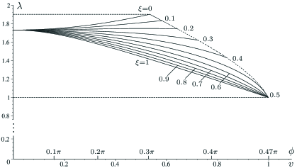
Figure 5: The relative frequency $\lambda=\omega_{r}/\Omega$ as a function of the angle $\phi$ and the velocity $v$ of particle circular motion for different values of the mixing parameter $\xi$.

For the scalar-vector superposition the dimensionless dynamical matrix is constructed as follows:

$$\bar{\cal D}^{(\xi)}=(1-\xi)\bar{\cal D}^{\rm(s)}+\xi\bar{\cal D}^{\rm(v)},$$ (A.57)

where $\xi$ is the mixing parameter. The relative frequency $\lambda$ is then calculated as a real positive root of the reduced secular equation $\det{\bar{\cal D}(\lambda)}=0$. In general, this can be done numerically.

In Fig. 5 the relative frequency $\lambda=\omega_{r}/\Omega$ as a function of the velocity $v$ of particle circular motion is shown for various values of the mixing parameter $\xi$. Let us note that

$$\lim\limits_{v\to 0}\frac{\omega_{r}}{\Omega}=\sqrt{3}$$

as it must be for the nonrelativistic problem with the linear potential $U=ar$ Duv12a .

References

- (1) E. Eichten, K. Gottfried, T. Kinoshita, J. Kogut, K. D. Lane, T.-M. Yan, Spectrum of Charmed Quark-Antiquark Bound States, Phys. Rev. Lett. 34, No 6, 369 372 (1975).
- (2) W. Lucha, F. F. Schoberl, D. Gromes, Bound states of quarks, Phys. Rep. 200, No 4, 127-240 (1991).
- (3) M. I. Haysak, V. I. Lengyel, Mass-spectrum of hadrons in the quasi-relativistic quark potential model, Ukr. J. Phys. 37, No 9, 1287-1301 (1992).
- (4) I. I. Haysak, V. S. Morokhovych, Hyperfine splitting and decay of heavy mesons, J. Phys. Studies 6, No 1, 55-59 (2002).
- (5) H. B. Nielsen, Dual strings, in Fundamentals of quark models, Proc. 17th Scot. Univ. Summer Sch. Phys., St.Andrews, Aug. 1976 (Edinburg, 1977), 465-547.
- (6) K. Johnson, C. Nohl, Simple semiclassical model for the rotational states of mesons containing massive quarks, Phys. Rev. D 19, No 1, 291-295 (1979).
- (7) Yu. Simonov, Ideas in nonperturbative QCD, Nuovo Cim. A 107, No 11, 2629-2644 (1994).
- (8) F. Bissey, A. I. Signal, Comparison of gluon flux-tube distribution for quark-diquark and quark-antiquark hadrons, Phys. Rev. D 80, No 11, 114506 (2009).
- (9) E. B. Berdnikov, G. P. Pronko, Relativistic model of orbital exitations of mesons, Sov. J. Nucl. Phys. 54, No 3(9), 763-776 (1991).
- (10) A. Duviryak, Application of two-body Dirac equation in meson spectroscopy, J. Phys. Studies 10, No 4, 290-314 (2006).
- (11) A. Duviryak, Solvable two-body Dirac equation as a potential model of light mesons, SIGMA 4, 048 (2008), 19 p.
- (12) C. Goebel, D. LaCourse, M. G. Olsson, Systematics of some ultrarelativistic potential models, Phys. Rev. D. 41, No 9, 2917-2923 (1990).
- (13) Y. S. Kim, M. E. Noz, Covariant harmonic oscillator and the quark model, Phys. Rev. D 8, No 10, 3521-3527 (1973).
- (14) T. Takabayasi, Relativistic mechanics of confined particles as extended model of hadrons, Suppl. Progr. Theor. Phys. 67, 1-68 (1979).
- (15) S. Ishida, M. Oda, A universal spring and meson orbital Regge trajectories, Nuovo Cim. A 107, No 11, 2519-2525 (1994).
- (16) I. I. Haysak, V. I. Lengyel, A. O. Shpenik, Fine splitting of two-quark systems from the Dirac equation. in Hadrons-94. Proc. of Workshop on Soft Physics (Strong Interaction at Large Distance), Uzhgorod, 1994, eds. G. Bugrij, L. Jenkovszky and E. Martynov, (Bogoliubov Institute for Theoretical Physics, Kiev, 1994), 267–271.
- (17) I. I. Haysak, V. I. Lengyel, A. O. Shpenik, S. Chalupka, M. Salak, Quark masses in the relativistic analytic model, Ukr. J. Phys. 4, No 3, 370-372 (1996).
- (18) V. Yu. Lazur, A. K. Reity, V. V. Rubish, Semiclassical approximation in the relativistic potential model of B and D mesons, Theor. Math. Phys. 155, No 3, 825 847 (2008).
- (19) H. W. Crater, P. Van Alstine, Relativistic naive quark model for spinning quarks in meson, Phys. Rev. Lett. 53, No 16, 1527-1530 (1984).
- (20) H. Sazdjian, Relativistic quarkonium dynamics, Phys. Rev. D 33, No 11, 3425-3434 (1986).
- (21) C. Semay, R. Ceuleneer, Two-body Dirac equation and Regge trajectories. Phys. Rev. D 48, No 9, 4361-4369 (1993).
- (22) H. W. Crater, P. Van Alstine, Relativistic calculation of the meson spectrum: A fullu covariant treatment versus standard treatments, Phys. Rev. D 70, No 3, 034026 (2004), 31p.
- (23) M. Moshinsky, A. G. Nikitin, The many body problem in relativistic quantum mechanics. Revista Mexicana de Física 50, 66-73 (2005); arXiv: hep-ph/0502028.
- (24) T. Biswas, F. Rohrlich, A relativistic quark model for hadrons, Nuovo Cim. A 88, No 2, 125-144 (1985); T. Biswas, F. Rohrlich, Fully relativistic hadron spectroscopy, Ibid, 145-160 (1985).
- (25) V. V. Kruschev, Mass spectrum of mesons in generalized quark field model, Sov. J. Nucl. Phys. 46, No 1(7), 219-225 (1987).
- (26) V. V. Kruschev, Mass formulae for mesons containing light quarks, Preprint IHEP 87-9 (Serpukhov, 1987).
- (27) V. V. Kruschev, Strange meson mass spectrum in relativistic model for quasi-independent quarks, Preprint IHEP 89-111 (Serpukhov, 1989).
- (28) A. Rivacoba, Fokker-action principle for a system of particles interacting through a linear potential, Nuovo Cimento B 84, No 1, 35-42 (1984).
- (29) J. Weiss, Is there action-at-a-distance linear confinement ? J. Math. Phys. 27, No 4, 1015-1022 (1986).
- (30) P. Havas, Galilei- and Lorentz-invariant particle systems and their conservation laws, in Problems in the Foundations of Physics (Springer, Berlin, 1971), 31-48.
- (31) E.H. Kerner (ed.) The Theory of Action-at-a-Distance in Relativistic Particle Mechanics, Collection of reprints (Gordon and Breach, New York, 1972).
- (32) A. Duviryak, Fokker-type confinement models from effective Lagrangian in classical Yang-Mills theory, Int. J. Mod. Phys. A 14, No 28, 4519-4547 (1999).
- (33) D. J. Louis-Martinez, Relativistic action at a distance and fields, Found. Phys. 42, No 2, 215-223 (2012).
- (34) R. P. Gaida, Yu. B. Kluchkovsky, V. I. Tretyak, Three-dimensional Lagrangian approach to the classical relativistic dynamics of directly interacting particles in Constraint’s Theory and Relativistic Dynamics, Florence (Italy), 1986, eds. G. Longhi and L. Lusanna (World Scientific Publishing Co., Singapore, 1987), 210-241.
- (35) X. Jaén, R. Jáuregui, J. Llosa, A. Molina, Hamiltonian formalism for path-dependent Lagrangians, Phys. Rev. D 36, No 8, 2385-2398 (1987).
- (36) X. Jaén, R. Jáuregui, J. Llosa, A. Molina, Canonical formalism for path-dependent Lagrangians. Coupling constant expansion, J. Math. Phys 30, No 12, 2807-2814 (1989).
- (37) J. Llosa, J. Vives, Hamiltonian formalism for nonlocal Lagrangians, J. Math. Phys. 35, No 6, 2856-2877 (1994).
- (38) 27. A. Duviryak. The time-asymmetric Fokker-type integrals and the relativistic Hamiltonian mechanics on the light cone, Acta Physica Polonica B 28, No 5, 1087-1109 (1997).
- (39) A. Duviryak, The two-particle time-asymmetric relativistic model with confinement interaction and quantization, Int. J. Mod. Phys. A 16, No 16, 2771-2788 (2001).
- (40) A. Duviryak, Quantization of almost-circular orbits in the Fokker action formalism. General scheme, arXiv:1210.5170.
- (41) J. A. Wheeler, R. P. Feynman, Classical electrodynamics in terms of direct interparticle action, Rev. Mod. Phys. 21, No 3, 425-433 (1949).
- (42) R.P. Gaida, Quasirelativistic interacting particle systems, Fiz. Elem. Chastits At. Yadra (USSR) 13, No 2, 427-93 (1982) [in Russian; Engl. transl in: Sov. J. Part. Nuclei (USA) 13, 179 (1982)].
- (43) J. Kiskis, Modified field theory for quark binding, Phys. Rev. D. 11, No 8, 2178-2202 (1975).
- (44) A. I. Alekseev, B. A. Arbuzov, V. A. Baikov, Infrared asymptotic behavior of gluon Green’s functions in quantum chromodynamics, Theor. Math. Phys. 52, No 2, 739-746 (1982).
- (45) A. I. Alekseev, B. A. Arbuzov, Classical Yang-Mills field theory with nonstandard Lagrangians, Theor. Math. Phys. 59, No 1, 372-378 (1984).
- (46) A. Katz, Alternative dynamics for classical relativistic particles, J. Math. Phys, 10, No 10, 1929-1931 (1969).
- (47) A. Schild, Electromagnetic two-body problem, Phys. Rev. 131, No 6, 2762-2766 (1963).
- (48) C. M. Andersen, H. C. von Baeyer, Circular orbits in classical relativistic two-body systems, Ann. Phys. (N.Y.), 60, No 1, 67-84 (1970).
- (49) A. Degasperis, Bohr quantization of relativistic bound states of two point particles, Phys. Rev. D 3, No 2, 273-279 (1971).
- (50) W. N. Herman, Formulation of Noether’s theorem for Fokker-type variational principles, J. Math. Phys. 26, No 11, 2769-2776 (1985).
- (51) B. Bakamjian, L. H. Thomas, Relativistic particle dynamics. II, Phys. Rev. 92, No 5, 1300-1310 (1953).
- (52) A. A. Duviryak, A class of canonical realizations of the Poincaré group, in Methods for studying differential and integral operators (Naukova Dumka, Kyß̈v, 1989), 59-66 [in Russian].
- (53) S. N. Sokolov, A. N. Shatnii, Physical equivalence of the three forms of relativistic dynamics and addition of interactions in the front and instant forms, Theor. Math. Phys. 37, No 3, 1029-1038 (1978).
- (54) W. N. Polyzou, Relativistic two-body models, Ann. Phys. 193, No 2, 367-418 (1989).
- (55) A. Duviryak, J. W. Darewych, Variational Hamiltonian treatment of partially reduced Yukawa-like models, J. Phys. A 37, No 34, 8365-8381 (2004).
- (56) P. Van Alstine, H. W. Crater, Wheeler-Feynman dynamics of spin- particles, Phys. Rev. D 33, No 4, 1037-1047 (1986).