Abstract

A unified framework to describe the adiabatic class of ensembles in the generalized statistical mechanics based on Schwämmle-Tsallis two parameter $(q,q^{\prime})$ entropy is proposed. The generalized form of the equipartition theorem, virial theorem and the adiabatic theorem are derived. Each member of the class of ensembles is illustrated using the classical nonrelativistic ideal gas and we observe that the heat functions could be written in terms of the Lambert’s $W$-function in the large $N$ limit. In the microcanonical ensemble we study the effect of gravitational field on classical nonrelativistic ideal gas and a system of hard rods in one dimension and compute their respective internal energy and specific heat. We found that the specific heat can take both positive and negative values depending on the range of the deformation parameters, unlike the case of one parameter Tsallis entropy.

PACS Number(s): 05.20.Gg, 05.70.Ce, 02.30.Gp
Keywords: Two parameter entropy, adiabatic class of ensembles, ideal gas, hard rods, gravity.

I Introduction

A system in thermodynamic equilibrium with its surroundings can be described using three macroscopic variables corresponding to the thermal, mechanical, and the chemical equilibrium. For each fixed value of these macroscopic variables (macrostate) we have many possible microscopic configurations (microstates). A collection of systems existing in the various possible microstates, but characterized by the same macroscopic variables is called an ensemble. The thermal, mechanical, and the chemical parameters can be choosen between either an extensive variable or an intensive variable and so, we have, in total eight different ensembles. The eight ensembles are further divided into two classes namely the isothermal class for which the thermal equilibrium variable is the temperature and the adiabatic class for which the thermal equilibrium variable is the heat function. The isothermal class comprises of the the canonical $(N,V,T)$, isothermal-isobaric $(N,P,T)$, grandcanonical $(\mu,V,T)$ and the generalized ensemble $(\mu,P,T)$. All the individual members of the adiabatic class of ensembles have same value for the heat function. The heat function is defined through the relation

$$\mathfrak{H}=E+\sum_{\{\ell\}}x_{\ell}X_{\ell},$$ (1.1)

where $E$ is the internal energy and the $x$ is an intensive thermodynamic variable whose conjugate extensive variable is $X$. Defining $\mathfrak{X}_{1}$ and $\mathfrak{X}_{2}$ as the variables corresponding to the chemical and mechanical equilibrium the specific form of each ensemble, its heat function and the corresponding entropy are listed in the Table 1.

Table 1: List of Adiabatic ensembles

		Heat function	Entropy
$\ell$	Ensemble	$\mathfrak{H}=E+\displaystyle{\sum_{\{\ell\}}}\,x_{\ell}X_{\ell}$	$S(\mathfrak{X}_{1},\mathfrak{X}_{2},\mathfrak{H})$
$0$	Microcanonical	$E$	$S(N,V,E)$
	$(N,V,E)$	(Internal energy)
$1$	Isoenthalpic - isobaric	$H=E+PV$	$S(N,P,H)$
	$(N,P,H)$	(Enthalpy)
$1$	Third adiabatic ensemble	$\mathsf{L}=E-\mu N$	$S(\mu,V,{\mathsf{L}})$
	$(\mu,V,\mathsf{L})$	(Hill energy)
$2$	Fourth adiabatic ensemble	$\mathsf{R}=E+PV-\mu N$	$S(\mu,P,{\mathsf{R}})$
	$(\mu,P,\mathsf{R})$	(Ray energy)

Of the four adiabatic ensembles, the microcanonical and the isoenthalpic-isobaric ensembles described in [[1]-[4]] are well known, but the other two ensembles namely $(\mu,V,\mathsf{L})$ and $(\mu,P,\mathsf{R})$ introduced through References [[5],[6]] are relatively less known. But they are important in studying adiabatically confined systems with variable number of particles. For example in Ref. [[7]] a Monte Carlo simulation of a system of liquid palladium has been carried out in the $(\mu,P,\mathsf{R})$ ensemble. The simulation was much more convenient in this ensemble and the results agreed with those obtained in the grandcanonical ensemble. Realizing the importance of classifying the ensembles, a unified treatment of the adiabatic ensembles was carried out in [[8]]. Later on the physical realizations corresponding to the eight ensembles and their interrelations through Laplace-Legendre transforms was studied in [[9]].

Tsallis proposed a generalization of the existing Boltzmann Gibbs statistical mechanics [[10]] through the introduction of $q$-deformed logarithm and exponential functions. The entropic expression in the generalized statistical mechanics was based on the $q$-deformed logarithm. Many other deformed entropies like the $\kappa$-entropy [[11]], the basic deformed entropies [[12]] etc., were also proposed. The equilibrium formulation of statistical mechanics based on the deformed entropies were developed and applied to a wide variety of systems like long range interacting rotators [[13]], relativistic gases [[14],[15]], and systems with long range microscopic memory [[16]]. Classification of the eight ensembles in to two different classes namely, the isothermal and the adiabatic class, and a unified description for each class in the framework of generalized statistical mechanics based on Tsallis $q$ entropy has been carried out in [[17]].

Later it was shown in [[18]] that an information theoretic entropy known as the Sharma-Taneja-Mittal entropy [[19],[20]] based on a two parameter logarithm was a natural generalization of both the Tsallis $q$-entropy and the $\kappa$-entropy. A study of nonlinear Fokker Planck equation corresponding to the two parameter $(r,s)$ Sharma-Taneja-Mittal entropy was carried out in [[21]] and the role played by the two parameters was investigated. One of the parameter ‘$r$’ was found to describe the nature of the stationary solution i.e., whether it is a weak stationary or a strong stationary solution and hence $r$ determines the degree of distortion of the usually obtained Gaussian distribution. The other parameter ‘$s$’ characterizes the dynamical properties of the transient solution and thus distinctly differentiates the regions of subdiffusion and superdiffusion. Investigation using the Lie symmetries [[22]] proved that the localized initial states are well approximated by the two parameter Gaussian rather than the standard Gaussian. The Sharma-Taneja-Mittal entropy is nonsymmetric with respect to its parameters, so with a view to provide a symmetric generalization of the Tsallis $q$ entropy, a two parameter logarithm and its inverse function the two parameter exponential were introduced in [[23]]. The doubly deformed $(q,q^{\prime})$ logarithm and its inverse the $(q,q^{\prime})$-exponential for a real variable $x$ are

$$\ln_{q,q^{\prime}}(x) = \frac{1}{1-q^{\prime}}\left[\exp\left(\frac{1-q^{\prime}}{1-q}(x^{1-q}-1)\right)-1\right],$$ (1.2)

$$\exp_{q,q^{\prime}}(x) = \left[1+\frac{1-q}{1-q^{\prime}}\ln\left(1+(1-q^{\prime})x\right)\right]^{\frac{1}{1-q}}.$$ (1.3)

The two parameter algebra based on the doubly deformed logarithm and the exponential was found [[24]] to be nondistributive in nature. Based on the definition of the two parameter logarithm $(\ref{2plog})$ the generalized entropy is

$$S_{q,q^{\prime}} = k_{{}_{TS}}\,\sum_{i=1}^{w}p_{i}\,\ln_{q,q^{\prime}}\left(\frac{1}{p_{i}}\right),$$ (1.4)

$$= \frac{k_{{}_{TS}}}{1-q^{\prime}}\,\sum_{i=1}^{w}p_{i}\,\left(\exp\left(\frac{1-q^{\prime}}{1-q}(p_{i}^{q-1}-1)\right)-1\right).$$

Under the assumption of equiprobability i.e., $p_{i}=1/w$ the two parameter entropy (1.4) reads:

$$S_{q,q^{\prime}}=\frac{k_{{}_{TS}}}{1-q^{\prime}}\,\left(\exp\left(\frac{1-q^{\prime}}{1-q}(w^{1-q}-1)\right)-1\right).$$ (1.5)

Both the doubly deformed logarithm (1.2) and the exponential (1.3) reduce to the respective one parameter logarithm or exponential defined in [[10]], when we let either $q$ or $q^{\prime}$ tend to unity. Due to this property, the Tsallis generalized entropy can be recovered by allowing either of the deformation parameters to approach it limiting value.

Nonextensivity has been proved to introduce effective interactions in ideal systems. In [[25]], we observed that an effective interaction was introduced between different degrees of freedom in an ideal diatomic gas molecule and in Ref. [[12]] it was clearly proved that the effect of basic deformation of a free ideal gas can be viewed as an effective interaction described by an Hamiltonian with logarithmic interactions. Recent simulational studies [[26]] show that classical collisions of a single ion in a radio frequency ion trap with an ideal gas generates non-Maxwellian distribution functions. Thus nonextensive statistical mechanics may be considered as a method to study interacting systems using noninteracting Hamiltonians, wherein the interactions are introduced through the nonextensivity in statistical mechanics. Taking this point of view, we feel that using a two parameter entropy gives us more freedom in introducing different forms of interactions both in terms of variety and their strengths. Throughout this article we take this spirit in investigating the ideal systems. Investigating the effect of a gravitational field on a system of ideal gas and one dimensional hard rods will help us in understanding the motion of a interacting gas cloud under the influence of gravity. We expect these calculations to correspond to some scenarios in which a massive object gravitationally attracts gas molecules from a gas cloud.

A canonical formulation of generalized statistical mechanics based on the two parameter entropy (1.4) was carried out in Ref. [[27]] and the authors found that the distribution could be obtained in terms of the Lambert’s $W$-function. This can be formally extended to describe the other members of the isothermal class of ensembles. In our current work we investigate the adiabatic class of ensembles of the generalized statistical mechanics based on the two parameter entropy. We provide a unified description of the adiabatic class and provide a two parameter generalization of the equipartition theorem, virial theorem and the adiabatic theorem. All the four ensembles are illustrated using the classical nonrelativistic ideal gas and their corresponding heat functions and heat capacities are obtained analytically. For the ideal gas, the phase space volume in the microcanonical and the isoenthalpic-isobaric ensemble can be found easily. To compute the respective heat function we need to adopt the large $N$ limit and the results are obtained in terms of the Lambert’s $W$-function. A brief introduction to the $W$-function is provided in Section II of this article. The phase space volume corresponding to the $(\mu,V,\mathsf{L})$ and the $(\mu,P,\mathsf{R})$ ensembles could not be evaluated exactly and we overcome this by using the large $N$ limit. Since the large $N$ limit has been already used in the computation of the phase space volume no further approximations are needed in the calculation of the heat function and the specific heat. The effect of gravity on a classical nonrelativistic ideal gas, and a system of one dimensional hard rod gas has been investigated [[28],[29]] in the extensive Boltzmann-Gibbs statistical mechanics. The authors found that the entropy is a decreasing function of the gravitational field indicating that gravity has an ordering effect in a thermodynamic system. In the present work we study the effect of a gravitational field in the framework of two parameter $(q,q^{\prime})$-entropy. First a $D$-dimensional nonrelativistic classical ideal gas confined in a finite region of space, subjected to an external gravitational field is investigated. The entropy and the specific heat are obtained exactly as a function of the internal energy. In the infinite height limit, the internal energy could be found only when we assume that the number of particles is very large. Next we study a system of one dimensional hard rods in the presence of gravity. Analogous to the classical ideal gas, the entropy and the specific heat are obtained as a function of internal energy. But in the infinite height limit the internal energy could be obtained as a function of temperature subject to the condition that the number of particles is very large. The heat capacities were found to admit both positive and negative values, in contrast to the previous results in [[30]] where the specific heat of a system of gas molecules in thermodynamic limit permits only negative values. Specific heats are supposed to characterize the amount of energy change when temperature is varied. Energy can both be liberated or absorbed depending on the interactions in the system as $T$ is varied. Our contention here is that with the $(q,q^{\prime})$ dependence the system exhibits effective interactions. The fact that specific heat can become negative for some range of $(q,q^{\prime})$ and may give clues about (i) Choosing the range of $(q,q^{\prime})$ for systems described by positive specific heat. (ii) If for a non-Boltzmann system with negative specific heat, it can help us to infer about interacting systems.

The plan of the article is as follows: Following the introduction in Section I we give a brief summary of the Lambert’s $W$ function in Section II. A unified description of the thermostatistical structure of all the four adiabatic ensembles is provided in Section III. In Section IV, we study all the four ensembles using classical nonrelativistic ideal gas, and each ensemble is treated separately in a subsection. The effect of an external gravitational field on thermodynamic system is studied in Section V. The first part of the section deals with the effect of gravity on a $D$-dimensional classical ideal gas. A system of one dimensional hard rod gas is examined in the second part of the section. The investigations are carried out in the microcanonical ensemble. We present our conclusions in Section V.

II Lambert’s W-function: a primer

A brief summary of the Lambert’s $W$-function and its mathematical properties is presented in the current section. Lambert’s $W$-function represented by $W(z)$ is defined as the multivalued inverse of the function $w\ e^{w}=z$ and satisfies the relation

$$W(z)\ e^{W(z)}=z,\qquad z\in\mathbb{C}.$$ (2.1)

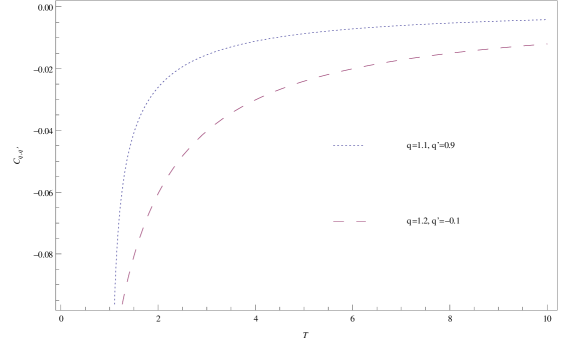
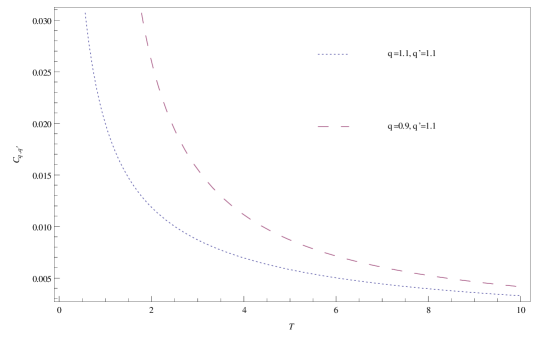
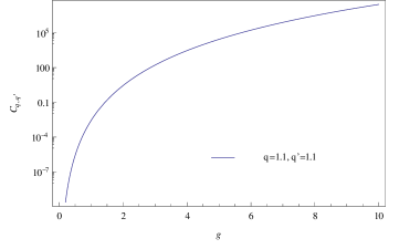
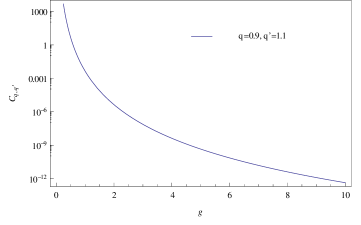
Figure 1: In the following graphs we plot the specific heat (5.31). In the first set of graphs above we plot the variation of the specific heat with respect to the temperature at a fixed value of the acceleration due to gravity. The second set of graphs consists of the variation of the specific heat with respect to the acceleration due to gravity at a fixed temperature. The values of $q$ and $q^{\prime}$ made use of are given in the graphs.

The various branches corresponding to the $W$-function are indexed by $k=0,\pm 1,\pm 2,...,$ and for real $z<-1/e$, the function $W(z)$ is always complex and multivalued. For real $z$ in the range $-1/e\leq z<0$, the function $W(z)$ comprises of two real branches namely $W_{0}(z)$ and $W_{-1}(z)$ represented by the solid line and the dotted line respectively in Figure 1. The branch $W_{0}(z)$ satisfies the condition $W(z)\geq-1$, and is generally known as the principal branch of the $W$ function. Correspondingly, when $W(z)\leq-1$ we have the $W_{-1}(z)$ branch.

Figure 1: A plot of the Lambert’s $W$ function $W(x)$ as a function of $x$.

The principal branch is analytic at $z=0$ and has the series expansion

$$W_{0}(z)=\sum_{n=1}^{\infty}\frac{(-n)^{n-1}}{n!}\,z^{n},$$ (2.2)

with a radius of convergence $e^{-1}$. Similarly the series corresponding to the branch $W_{-1}$ is

$$W_{-1}(z)=\sum_{n=0}^{\infty}c_{n}\,f^{n}(z);\qquad\qquad f(z)=\sqrt{2\ (ez+1)},$$ (2.3)

where the expansion coefficients can be computed from the recurrence relations

$$c_{k} = \frac{k-1}{k+1}\,\left(\frac{c_{k-2}}{2}+\frac{d_{k-2}}{4}\right)-\frac{d_{k}}{2}-\frac{c_{k-1}}{k+1},\qquad d_{k}=\sum_{j=2}^{k-1}c_{j}\,c_{k+1-j},$$ (2.4)

$$c_{0} = -1,\qquad c_{1}=1,\qquad d_{0}=2,\qquad d_{1}=-1.$$ (2.5)

The series converges for $-1/e\leq z<0$, which covers the whole domain of the $W_{-1}$ branch. From (2.1) the derivative of the $W$ function is found

$$W^{\prime}(z)=\frac{W(z)}{z\ (1+W(z))}.$$ (2.6)

In the current article physical requirements restricts our choice of the $W$ function to the principal branch. An excellent introduction to the Lambert’s $W$-function and its applications to engineering problems is discussed in [[31]]. Recently in signal processing the role of the $W_{-1}$ branch was analyzed [[32]]. The Lambert’s function has been used in the study of both classical [[33]] and quantum statistical mechanics [[34],[35]]. It also occurs [[36]] in the study of Fokker Planck equation in the small noise limit.

III Adiabatic ensemble: Generalized formulation

The individual members of an adiabatic ensemble have the same value of the heat function though they can be at different temperatures. For a system in thermodynamic equilibrium, there are four different adiabatic ensembles namely the microcanonical ensemble $(N,V,U)$, the isoenthalpic-isobaric ensemble $(N,P,H)$, the adiabatic ensemble with number fluctuations $(\mu,V,\mathsf{L})$, and the adiabatic ensemble with both number and volume fluctuations $(\mu,P,\mathsf{R})$. The microstate of a system of $N$ particles can be represented by a single point in the $2DN$ dimensional phase space. Corresponding to a particular value of the heat function which is a macrostate, we have a huge number of microstates. We need to compute the total number of microstates since it is a measure of the entropy. The points denoting the microstate of the system lie so close to each other that the surface area of the constant heat function curve in the phase space is regarded as a measure of the total number of microstates. For a system described by a Hamiltonian $\mathcal{H}$ the surface area corresponding to a constant heat function $\mathfrak{H}$ curve can be calculated from

$$\Omega(\mathfrak{X}_{1},\mathfrak{X}_{2},\mathfrak{H})=\sum_{X_{\{\ell\}}}\,\frac{1}{N!\,h^{DN}}\int_{r_{i}}\int_{p_{i}}\delta\Big{(}\mathcal{H}+\sum_{\{\ell\}}x_{\ell}X_{\ell}-{\mathfrak{H}}\Big{)}\prod_{i=1}^{N}{\rm d}^{D}r_{i}\,{\rm d}^{D}p_{i}.$$ (3.1)

Similarly the phase space volume enclosed by the constant heat function ${\mathfrak{H}}$ curve is

$$\varSigma(\mathfrak{X}_{1},\mathfrak{X}_{2},\mathfrak{H})=\sum_{X_{\{\ell\}}}\,\frac{1}{N!\,h^{DN}}\int_{r_{i}}\int_{p_{i}}\Theta\Big{(}\mathcal{H}+\sum_{\{\ell\}}x_{\ell}X_{\ell}-{\mathfrak{H}}\Big{)}\prod_{i=1}^{N}{\rm d}^{D}r_{i}\,{\rm d}^{D}p_{i},$$ (3.2)

where $\Theta$ is the Heaviside step function. Computation of the volume of the constant heat function curve assumes significance because of the difficulty in calculating the area of the curve. The volume enclosed by the phase space curve and its surface area are related via the expression

$$\Omega(\mathfrak{X}_{1},\mathfrak{X}_{2},\mathfrak{H})=\frac{\partial}{\partial\mathfrak{H}}\varSigma(\mathfrak{X}_{1},\mathfrak{X}_{2},\mathfrak{H}).$$ (3.3)

Since the phase space volume is a measure of the number of the microstates of the system, the two parameter entropy can be directly obtained from the knowledge of $\varSigma(\mathfrak{X}_{1},\mathfrak{X}_{2},\mathfrak{H})$ via the relation

$$S_{q,q^{\prime}}(\mathfrak{X}_{1},\mathfrak{X}_{2},\mathfrak{H})=k\;\ln_{q,q^{\prime}}\varSigma(\mathfrak{X}_{1},\mathfrak{X}_{2},\mathfrak{H}).$$ (3.4)

For a given adiabatic ensemble the temperature is defined via the relation

$$T=\left(\frac{\partial S_{q,q^{\prime}}}{\partial{\mathfrak{H}}}\right)^{-1}=\frac{(\varSigma(\mathfrak{X}_{1},\mathfrak{X}_{2},\mathfrak{H}))^{{}^{q}}}{k\;\Omega(\mathfrak{X}_{1},\mathfrak{X}_{2},\mathfrak{H})\,\exp\left(\frac{1-q^{\prime}}{1-q}((\varSigma(\mathfrak{X}_{1},\mathfrak{X}_{2},\mathfrak{H}))^{1-q}-1)\right)}.$$ (3.5)

Using the definition of the temperature (3.5), the phase space volume (3.2) and the surface area (3.1), we can calculate the expression corresponding to the heat function. From the expression for the heat function the specific heat can be calculated through the relation

$$C_{x_{\{\ell\}}}=\frac{\partial{\mathfrak{H}}_{q}}{\partial T}\bigg{|}_{x_{\{\ell\}}}.$$ (3.6)

For any adiabatic ensemble the expectation value of an observable $O$ is defined as

$$\langle O\rangle=\frac{1}{\Omega(\mathfrak{X}_{1},\mathfrak{X}_{2},\mathfrak{H})}\,\sum_{X_{\{\ell\}}}\frac{1}{N!\,h^{DN}}\,\int_{r_{i}}\int_{p_{i}}O\;\;\delta\Big{(}\mathcal{H}+\sum_{\{\ell\}}x_{\ell}X_{\ell}-{\mathfrak{H}}\Big{)}\prod_{i=1}^{N}{\rm d}^{D}r_{i}\,{\rm d}^{D}p_{i}.$$ (3.7)

The above expression is extremely useful in computing the average energy in the $(N,P,H)$, $(\mu,V,\mathsf{L})$ and the $(\mu,P,\mathsf{R})$ ensembles. By using the suitable Legendre transformations, the average energy can also be obtained from the heat functions corresponding to these ensembles. From the entropy the extensive thermodynamic quantities whose conjugate intensive variables are held fixed can be computed through the relation

$$X_{\ell}(\mathfrak{X}_{1},\mathfrak{X}_{2},\mathfrak{H})=-\frac{1}{\beta}\;\frac{\partial}{\partial x_{\ell}}\,S(\mathfrak{X}_{1},\mathfrak{X}_{2},\mathfrak{H}).$$ (3.8)

The equipartition theorem is derived in a unified manner for all the four adiabatic ensembles in the framework of generalized statistical mechanics based on the Schwämmle-Tsallis $(q,q^{\prime})$ entropy. Representing the phase space variables $r_{i}$ and $p_{i}$ $(i=1,2,...,3N)$ by a common variable $y_{i}$, we find the following expectation value

$$\bigg{\langle}y_{i}\;\frac{\partial{\mathcal{H}}}{\partial y_{j}}\bigg{\rangle}=kT\;\left(\varSigma(\mathfrak{X}_{1},\mathfrak{X}_{2},\mathfrak{H})\right)^{1-q}\;\exp\left(\frac{1-q^{\prime}}{1-q}((\varSigma(\mathfrak{X}_{1},\mathfrak{X}_{2},\mathfrak{H}))^{1-q}-1)\right)\delta_{ij},$$ (3.9)

which is a generalization of the equipartition function. We notice that the $(q,q^{\prime})$ generalized equipartition theorem is dependent on the phase space volume in contrast to the extensive Boltzmann-Gibbs statistics. This observation is in line with the earlier result obtained for the Tsallis entropy in Ref. [[17]] and yields the Boltzmann-Gibbs limit when both the nonextensive parameters $q$ and $q^{\prime}$ are set to unity. When we let the variable $y_{i}$ to be the coordinate $r_{i}$ and invoke the Dirac delta function, we get a specific form of the equipartition theorem:

$$\bigg{\langle}r_{i}\;\frac{\partial{\mathcal{H}}}{\partial r_{i}}\bigg{\rangle}\equiv-\langle r_{i}\,\dot{p}_{i}\rangle=\langle r_{i}\,F_{i}\rangle = kT\;\left(\varSigma(\mathfrak{X}_{1},\mathfrak{X}_{2},\mathfrak{H})\right)^{1-q}$$ (3.10)

$$\exp\left(\frac{1-q^{\prime}}{1-q}((\varSigma(\mathfrak{X}_{1},\mathfrak{X}_{2},\mathfrak{H}))^{1-q}-1)\right).$$

Similarly when we set $y_{i}$ to be equal to $p_{i}$ the momentum variable we obtain

$$\bigg{\langle}p_{i}\,\frac{\partial{\mathcal{H}}}{\partial p_{i}}\bigg{\rangle}\equiv\langle p_{i}\,\dot{r}_{i}\rangle=kT\,\left(\varSigma(\mathfrak{X}_{1},\mathfrak{X}_{2},\mathfrak{H})\right)^{1-q}\,\exp\left(\frac{1-q^{\prime}}{1-q}((\varSigma(\mathfrak{X}_{1},\mathfrak{X}_{2},\mathfrak{H}))^{1-q}-1)\right).$$ (3.11)

Through a canonical transformation, sometimes the Hamiltonian of a system can be written in the following form $\mathcal{H}=\sum_{i}(A_{i}\ P_{i}^{2}+B_{i}\ Q_{i}^{2})$. Aided by equations (3.10) and (3.11) we find the expectation value of such an Hamiltonian to be

$$\langle\mathcal{H}\rangle=DN\,kT\,\left(\varSigma(\mathfrak{X}_{1},\mathfrak{X}_{2},\mathfrak{H})\right)^{1-q}\,\exp\left(\frac{1-q^{\prime}}{1-q}((\varSigma(\mathfrak{X}_{1},\mathfrak{X}_{2},\mathfrak{H}))^{1-q}-1)\right).$$ (3.12)

A two parametric generalization of the virial theorem could be obtained from the relation (3.10) and reads:

$$\bigg{\langle}\sum_{i}^{DN}r_{i}\,\dot{p}_{i}\bigg{\rangle}=-DN\,kT\,\left(\varSigma(\mathfrak{X}_{1},\mathfrak{X}_{2},\mathfrak{H})\right)^{1-q}\,\exp\left(\frac{1-q^{\prime}}{1-q}((\varSigma(\mathfrak{X}_{1},\mathfrak{X}_{2},\mathfrak{H}))^{1-q}-1)\right).$$ (3.13)

Below we verify the adiabatic theorem for the generalized statistical mechanics based on the two parameter entropy. Let us consider the Hamiltonian to contain an external parameter $a$, in addition to the phase space co-ordinates. An expectation value of the derivative of the Hamiltonian with respect to the external parameter yields the thermodynamic conjugate variable $f$ corresponding to the parameter $a$

$$\bigg{\langle}\frac{\partial\mathcal{H}}{\partial a}\bigg{\rangle} = \frac{1}{\Omega(\mathfrak{X}_{1},\mathfrak{X}_{2},\mathfrak{H})}\sum_{X_{\ell}}\frac{1}{N!\,h^{DN}}\,\int_{r_{i}}\int_{p_{i}}\left(\frac{\partial\mathcal{H}}{\partial a}\right)\delta(\mathcal{H}+\sum_{X_{\ell}}x_{\ell}X_{\ell}-\mathfrak{H})\prod_{i=1}^{N}d^{D}r_{i}\,d^{D}p_{i},$$ (3.14)

$$= \frac{\partial\mathfrak{H}}{\partial a}=f.$$

The description of the adiabatic ensembles given above has been illustrated through certain examples. First we consider a classical ideal gas and provide an analytic solution to the specific heat in all the four ensembles by using a large $N$ approximation. Later on we study a microcanonical $D$-dimensional classical ideal gas under the influence of gravity and compute its specific heat. Finally we investigate a hard rod gas under gravity in the framework of microcanonical ensemble.

IV Application - Classical ideal gas

The Hamiltonian of a nonrelativistic classical ideal gas in $D$ dimensions is

$$\mathcal{H}=\sum_{i}\frac{p_{i}^{2}}{2m},\qquad p_{i}=|{\bf{p}}_{i}|,$$ (4.1)

where ${\bf{p}}_{i}$ for $(i=1,2,...,N)$ represent the $D$-dimensional momenta of the gas molecules. In this section we find the phase space volume corresponding to this Hamiltonian for all the four ensembles. From the phase space volume we derive the relevant thermodynamic quantities like the entropy, the heat function and the heat capacity.

A. Microcanonical ensemble

The classical nonrelativistic ideal gas described by (4.1) is studied in the microcanonical ensemble. In order to compute the entropy of the system, we calculate the phase space volume enclosed by the constant energy curve. Substituting the expression of the Hamiltonian in (3.2)

$$\varSigma(N,V,E)=\frac{1}{N!\,h^{DN}}\;\int_{r_{i}}\int_{p_{i}}\Theta\left(\sum_{i}\frac{p_{i}^{2}}{2m}-E\right)\;\prod_{i=1}^{N}{\rm d}^{D}r_{i}\,{\rm d}^{D}p_{i}.$$ (4.2)

The phase space integral is computed in the following manner: First we notice that the momentum integration is the volume of a $DN$-dimensional sphere of radius $\sqrt{2mE}$. Next we integrate over the position co-ordinates to obtain the phase space volume in the microcanonical ensemble

$$\varSigma(N,V,E)=\frac{V^{N}}{N!}\;\frac{\mathcal{M}^{N}}{\Gamma\left(\frac{DN}{2}+1\right)}\;E^{\frac{DN}{2}},$$ (4.3)

where we define $\mathcal{M}=(2\pi m/h^{2})^{D/2}$ for the sake of convenience. The corresponding surface area enclosed by the phase space curve is

$$\Omega(N,V,E)=\frac{V^{N}}{N!}\;\frac{\mathcal{M}^{N}}{\Gamma\left(\frac{DN}{2}\right)}\;E^{\frac{DN}{2}-1}.$$ (4.4)

The microcanonical entropy of a classical ideal gas obtained from the knowledge of the phase space volume (4.3) reads:

$$S_{q,q^{\prime}}=\frac{k}{1-q^{\prime}}\;\left[\exp\left(\frac{1-q^{\prime}}{1-q}\big{(}(\Xi_{mc}\;E^{\frac{DN}{2}})^{1-q}-1\big{)}\right)-1\right],$$ (4.5)

where the factor $\Xi_{mc}$ is defined as

$$\Xi_{mc}=\frac{V^{N}}{N!}\;\frac{\mathcal{M}^{N}}{\Gamma\left(\frac{DN}{2}+1\right)}.$$ (4.6)

In the limit $(q,q^{\prime})\rightarrow 1$, we recover the extensive Boltzmann Gibbs entropy. From the definition of temperature (3.5), we arrive at the following expression

$$\frac{1}{T}=\frac{DN}{2}\,k\;\Xi_{mc}^{1-q}\,E^{(1-q)\,\frac{DN}{2}-1}\,\exp\left(\frac{1-q^{\prime}}{1-q}\big{(}(\Xi_{mc}\;E^{\frac{DN}{2}})^{1-q}-1\big{)}\right).$$ (4.7)

Inversion of the above relation (4.7), to obtain the internal energy is intractable and so, we look into the naturally occurring large $N$ limit. In this limit we can safely neglect the factor of one in comparison with $(1-q)DN/2$ and this enables us to make the following approximation $E^{(1-q)\,{\frac{DN}{2}}-1}\approx E^{(1-q)\,{\frac{DN}{2}}}$. For very large values of $N$ the deformation parameter $(1-q)$ should be $O(1/N)$ for the factor $1$ to make a reasonable contribution. Using the assumption outlined above we get

$$\exp\left(\frac{1-q^{\prime}}{1-q}\right)\frac{2}{DN\,k\,T}=\Xi_{mc}^{1-q}\,E^{(1-q)\,\frac{DN}{2}}\,\exp\left(\frac{1-q^{\prime}}{1-q}\,(\Xi_{mc}\;E^{\frac{DN}{2}})^{1-q}\right).$$ (4.8)

The inversion of the above function leads to an expression of the internal energy in terms of the Lambert’s $W$ function as

$$E=\left[\frac{1-q}{1-q^{\prime}}\;\frac{1}{\Xi_{mc}^{1-q}}\;W_{0}\left(\frac{1-q^{\prime}}{1-q}\,\exp\left(\frac{1-q^{\prime}}{1-q}\right)\frac{2\beta}{DN}\right)\right]^{\frac{2}{(1-q)\,DN}}.$$ (4.9)

The requirement that the entropy be concave decides the range of the deformation parameters. From the discussion in Ref. [[23]], we notice that the entropy is concave in the region $q+q^{\prime}\geq 1$ excluding the region $0\leq(q,q^{\prime})\leq 1$, where the entropy does not have fixed curvature sign. The argument of the $W$ function in (4.9) is positive in the region (a) for which $q>1$ and $q^{\prime}>1$, and hence the energy in this region is characterized by the principal branch. Under the restriction $q+q^{\prime}<1$, there are two other major regions namely, (b) $q>1$ and $-\infty<q^{\prime}<1$ and (c) $q^{\prime}>1$ and $-\infty<q<1$ in which the argument of the $W$ function is negative. Though we have a choice between the $W_{0}$ and the $W_{-1}$ branch, the continuity requirement on energy restricts our choice to the $W_{0}$ branch. Thus we conclude that only the principal branch contributes in the definition of energy. In all the subsequent discussions in this article, we maintain the definition of the regions (a), (b) and (c) as described above. The specific heat at constant volume evaluated from the internal energy is

$$C_{V}\equiv\frac{\partial E}{\partial T}=-\frac{k\,\beta}{(1-q)\,DN/2}\;\frac{W_{0}(\mathsf{b}\,\beta)}{1+W_{0}(\mathsf{b}\,\beta)}\;\left[\mathsf{a}\,W_{0}(\mathsf{b}\,\beta)\right]^{\frac{1-(1-q)DN/2}{(1-q)DN/2}},$$ (4.10)

where the factors $\mathsf{a}$ and $\mathsf{b}$ are as defined below:

$$\mathsf{a}=\frac{1-q}{1-q^{\prime}}\;\frac{1}{\Xi_{mc}^{1-q}},\qquad\mathsf{b}=\frac{1-q^{\prime}}{1-q}\,\exp\left(\frac{1-q^{\prime}}{1-q}\right)\frac{2}{DN}.$$ (4.11)

Invoking the large $N$ limit in the final expression of the specific heat we arrive at

$$C_{V}=-\frac{k\,\beta}{(1-q)\,DN/2}\;\frac{1}{\mathsf{a}(1+W_{0}(\mathsf{b}\,\beta))}.$$ (4.12)

From the expression of the specific heat (4.12), we notice that it can be either positive or negative depending on the values of the deformation parameters $q$ and $q^{\prime}$. In the region (a) and region (c) the specific heat is positive, whereas in the region (b) it is negative. We do not recover the Boltzmann Gibbs statistics from our above calculations, because in the computation of energy (4.9), we have made use of the large $N$ limit which does not commute with extensive $(q,q^{\prime})\rightarrow 1$ limit.

B. Isoenthalpic-isobaric ensemble

A system which exchanges internal energy and volume with its surroundings in such a way that its enthalpy remains constant is described by the isoenthalpic-isobaric ensemble. In order to calculate the thermodynamic quantities we first find the phase space volume enclosed by the constant enthalpy curve. The integral expression corresponding to the phase space volume is

$$\varSigma(N,P,H)=\sum_{V}\frac{1}{N!\,h^{DN}}\;\int_{r_{i}}\int_{p_{i}}\Theta\left(\sum_{i}\frac{p_{i}^{2}}{2m}+PV-H\right)\;\prod_{i=1}^{N}{\rm d}^{D}r_{i}\,{\rm d}^{D}p_{i}.$$ (4.13)

Using the fact that the momentum integration is nothing but geometrically equivalent to a $DN$ dimensional sphere of radius $\sqrt{2m(H-PV)}$, and integrating over the position co-ordinates we arrive at

$$\varSigma(N,P,H)=\frac{\mathcal{M}^{N}}{N!}\;\frac{1}{\Gamma\left(\frac{DN}{2}+1\right)}\;\sum_{V}V^{N}(H-PV)^{\frac{DN}{2}}.$$ (4.14)

In the next step we consider a summation over the volume eigenstates. Since the volume states are very closely spaced the summation is replaced by an integration. But an integral over the volume leads to over counting of the eigenstates. To overcome this we employ the shell particle method of counting volume states developed in [[37],[38]]. In this method we take into account only the minimum volume needed to confine a particular configuration. The minimum volume needed to confine a particular configuration is found by imposing a condition wherein we require atleast one particle to lie on the boundary of the system. All the equivalent ways of choosing a minimum volume for a particular configuration is treated as the same volume eigenstate and is considered only once. Using this shell particle technique to reject the redundant volume states we arrive at

$$\varSigma(N,P,H)=\mathcal{M}^{N}\;\left(\frac{1}{P}\right)^{N}\;\frac{H^{\mathfrak{D}}}{\Gamma({\mathfrak{D}}+1)},\qquad\mathfrak{D}=\frac{DN}{2}+N.$$ (4.15)

A similar evaluation of the surface area enclosed by the curve of constant enthalpy yields

$$\Omega(N,P,H)=\mathcal{M}^{N}\;\left(\frac{1}{P}\right)^{N}\;\frac{H^{{\mathfrak{D}}-1}}{\Gamma({\mathfrak{D}})}.$$ (4.16)

From the knowledge of the phase space volume (4.15), the entropy of a classical ideal gas in the isoenthalpic-isobaric ensemble is found:

$$S_{q,q^{\prime}}=\frac{k}{1-q^{\prime}}\;\left[\exp\left(\frac{1-q^{\prime}}{1-q}\big{(}(\Xi_{ie}\;{H^{\mathfrak{D}}})^{1-q}-1\big{)}\right)-1\right].$$ (4.17)

The Boltzmann Gibbs entropy is recovered in the limit $(q,q^{\prime})\rightarrow 1$. The factor $\Xi_{ie}$ used in the above equation is

$$\Xi_{ie}=\mathcal{M}^{N}\;\left(\frac{1}{P}\right)^{N}\;\frac{1}{\Gamma({\mathfrak{D}}+1)}.$$ (4.18)

The partial derivative of the entropy (4.17) with respect to the enthalpy gives the temperature of the isoenthalpic-isobaric ensemble

$$\frac{1}{T}={\mathfrak{D}}\,k\,\Xi_{ie}^{1-q}\,H^{(1-q)\,{\mathfrak{D}}-1}\,\exp\left(\frac{1-q^{\prime}}{1-q}\big{(}(\Xi_{ie}\;{H^{\mathfrak{D}}})^{1-q}-1\big{)}\right).$$ (4.19)

In order to invert the above equation we assume the large $N$ limit and this consequently leads to the approximation that $H^{(1-q)\,{\mathfrak{D}}-1}\approx H^{(1-q)\,{\mathfrak{D}}}$. Rewriting the equation (4.19) based on the assumption yields the expression

$$\exp\left(\frac{1-q^{\prime}}{1-q}\right)\frac{1}{{\mathfrak{D}}\,k\,T}=\Xi_{ie}^{1-q}\,H^{(1-q)\,{\mathfrak{D}}}\,\exp\left(\frac{1-q^{\prime}}{1-q}\,(\Xi_{ie}\;{H^{\mathfrak{D}}})^{1-q}\right).$$ (4.20)

The solution of the above equation yields the enthalpy in terms of the Lambert’s $W$-function

$$H=\left[\frac{1-q}{1-q^{\prime}}\;\frac{1}{\Xi_{ie}^{1-q}}\;W_{0}\left(\frac{1-q^{\prime}}{1-q}\,\exp\left(\frac{1-q^{\prime}}{1-q}\right)\frac{\beta}{{\mathfrak{D}}}\right)\right]^{\frac{1}{(1-q){\mathfrak{D}}}}.$$ (4.21)

The requirement that the entropy should be concave, along with the fact that the enthalpy is a continuous function restricts our choice of the $W$ function to the principal branch. The specific heat at constant pressure computed from the enthalpy (4.21) is

$$C_{P}\equiv\frac{\partial H}{\partial T}=-\frac{k\,\beta}{(1-q)\,{\mathfrak{D}}}\;\frac{W_{0}(\mathfrak{b}\,\beta)}{1+W_{0}(\mathfrak{b}\,\beta)}\;\left[\mathfrak{a}\,W_{0}(\mathfrak{b}\,\beta)\right]^{\frac{1-(1-q){\mathfrak{D}}}{(1-q){\mathfrak{D}}}},$$ (4.22)

where, the factors $\mathfrak{a}$ and $\mathfrak{b}$ are as defined below:

$${\mathfrak{a}}=\frac{1-q}{1-q^{\prime}}\;\frac{1}{\Xi_{ie}^{1-q}},\qquad{\mathfrak{b}}=\frac{1-q^{\prime}}{1-q}\,\exp\left(\frac{1-q^{\prime}}{1-q}\right)\frac{1}{{\mathfrak{D}}}.$$ (4.23)

In the large $N$ limit the expression for the heat capacity reads:

$$C_{P}=-\frac{k\,\beta}{(1-q)\,{\mathfrak{D}}}\;\frac{1}{{\mathfrak{a}}(1+W_{0}(\mathfrak{b}\,\beta))}.$$ (4.24)

The specific heat is positive in the regions (a) and (c) and negative in the region (b). Since we adopted the large $N$ limit in evaluating the enthalpy (4.21) we do not recover the corresponding Boltzmann Gibbs result, because the extensive limit and the large $N$ limit do not commute with each other.

C. $(\mu,V,\mathsf{L})$ ensemble

The Hill energy $\mathsf{L}$ is the heat function corresponding to the $(\mu,V,\mathsf{L})$ ensemble. The phase space volume enclosed by the curve of constant Hill energy $\mathsf{L}$ is

$$\varSigma(\mu,V,\mathsf{L})=\sum\frac{1}{N!\,h^{DN}}\;\int_{r_{i}}\int_{p_{i}}\Theta\left(\sum_{i}\frac{p_{i}^{2}}{2m}-\mu N-\mathsf{L}\right)\;\prod_{i=1}^{N}{\rm d}^{D}r_{i}\,{\rm d}^{D}p_{i}.$$ (4.25)

Integrating over the phase space variables $p_{i}$ and $r_{i}$, we arrive at

$$\varSigma(\mu,V,\mathsf{L})=\sum_{N=0}^{\infty}\frac{V^{N}}{N!}\;\frac{\mathcal{M}^{N}}{\Gamma\left(\frac{DN}{2}+1\right)}\;(\mathsf{L}+\mu N)^{\frac{DN}{2}}.$$ (4.26)

An exact evaluation of the summation given in (4.26) could not be achieved. In order to calculate an approximate value in the large $N$ limit we carry out the following procedure. First we approximate the factor $(\mathsf{L}+\mu N)^{\frac{DN}{2}}$ as follows

$$(\mathsf{L}+\mu N)^{\frac{DN}{2}} = (\mu N)^{\frac{DN}{2}}\,\left(1+\frac{\mathsf{L}}{\mu N}\right)^{\frac{DN}{2}},$$ (4.27)

$$= (\mu N)^{\frac{DN}{2}}\,\exp\left(\frac{DN}{2}\ln\left(1+\frac{\mathsf{L}}{\mu N}\right)\right).$$

For very small values of $x$ we can make use of the approximation $\ln(1+x)\approx x$ and this leads to

$$(\mathsf{L}+\mu N)^{\frac{DN}{2}}=(\mu N)^{\frac{DN}{2}}\exp\left(\frac{D}{2}\,\frac{\mathsf{L}}{\mu}\right).$$ (4.28)

In the next step we use the Stirling’s approximation for the gamma function as given below:

$$\Gamma\left(\frac{DN}{2}+1\right)\approx\left(\frac{DN}{2}\right)^{\frac{DN}{2}}\exp\left(-\frac{DN}{2}\right).$$ (4.29)

Substituting the relations (4.28), and (4.29) in (4.26) we arrive at

$$\varSigma(\mu,V,\mathsf{L})=\exp\left(\frac{D}{2}\,\frac{\mathsf{L}}{\mu}\right)\;\sum_{N=0}^{\infty}\;\frac{V^{N}}{N!}\;\frac{\mathcal{M}^{N}}{\left(\frac{DN}{2}\right)^{\frac{DN}{2}}\exp\left(-\frac{DN}{2}\right)}\;(\mu N)^{\frac{DN}{2}}.$$ (4.30)

Now the summation over $N$ can be carried out in (4.30), enabling us to write the approximate expression for the phase space volume

$$\varSigma(\mu,V,\mathsf{L})=\exp\left(\frac{D}{2}\,\frac{\mathsf{L}}{\mu}\right)\;\exp\left(\frac{V\,\mu^{D/2}\,e^{D/2}\,\mathcal{M}}{(D/2)^{D/2}}\right).$$ (4.31)

The approximate computation used by us to calculate the phase space volume (4.31) can be considered as a first order approximation of the summation in (4.26). Similarly the surface area enclosed by the curve of constant ${\mathsf{L}}$ is also found

$$\Omega(\mu,V,\mathsf{L})=\frac{D}{2\mu}\;\exp\left(\frac{D}{2}\,\frac{\mathsf{L}}{\mu}\right)\;\exp\left(\frac{V\,\mu^{D/2}\,e^{D/2}\,\mathcal{M}}{(D/2)^{D/2}}\right).$$ (4.32)

The entropy of the classical ideal gas in this adiabatic ensemble found from (4.31) is

$$S_{q,q^{\prime}}=\frac{k}{1-q^{\prime}}\;\left[\exp\left(\frac{1-q^{\prime}}{1-q}\left(\left(\Xi_{he}\;\exp\left(\frac{D}{2}\,\frac{\mathsf{L}}{\mu}\right)\right)^{1-q}-1\right)\right)-1\right],$$ (4.33)

where, for the sake of convenience we define:

$$\Xi_{he}=\exp\left(\frac{V\,\mu^{D/2}\,e^{D/2}\,\mathcal{M}}{(D/2)^{D/2}}\right).$$ (4.34)

The temperature of this ensemble calculated from the defining relation (3.5) is

$$\frac{1}{T}=\frac{D}{2\mu}\,k\,\Xi_{he}^{1-q}\,\left(\exp\left(\frac{D}{2}\,\frac{\mathsf{L}}{\mu}\right)\right)^{1-q}\exp\left(\frac{1-q^{\prime}}{1-q}\left(\left(\Xi_{he}\;\exp\left(\frac{D}{2}\,\frac{\mathsf{L}}{\mu}\right)\right)^{1-q}-1\right)\right).$$ (4.35)

Rewriting (4.35) we immediately recognize it as the equation whose solution is given by the Lambert’s $W$-function. Thus the Hill energy in terms of the $W$-function reads:

$$\mathsf{L}=\frac{2\,\mu}{(1-q)\,D}\;\ln\left[\frac{1-q}{1-q^{\prime}}\;\frac{1}{\Xi_{he}^{1-q}}\;W_{0}\left(\frac{1-q^{\prime}}{1-q}\,\exp\left(\frac{1-q^{\prime}}{1-q}\right)\frac{2\,\beta\mu}{D}\right)\right].$$ (4.36)

The principal branch of the $W$ function is chosen based on the concavity requirement on the entropy and the continuity of the Hill energy. The Hill energy $\mathsf{L}$ is uniformly positive in the region (c) for which $q^{\prime}>1$ and $-\infty<q<1$, whereas in the other two regions (b) and (c) it is positive only when the argument of the logarithm is less than $1$. From (4.36) the specific heat at constant volume is found

$$C_{V}\equiv\frac{\partial\mathsf{L}}{\partial T}=-\frac{\mu}{(1-q)D/2}\,\frac{k\beta}{1+W_{0}(\mathtt{b}\,\beta)},\qquad\mathtt{b}=\frac{1-q^{\prime}}{1-q}\,\exp\left(\frac{1-q^{\prime}}{1-q}\right)\,\frac{\mu}{D/2}.$$ (4.37)

Subject to the condition $q+q^{\prime}>1$ and excluding the region $0\leq(q,q^{\prime})\leq 1$, the specific heat is positive in the region $q>1$ and negative in the region $q<1$. Due to the noncommutative nature of the extensive limit and the large $N$ limit, we are unable to recover the Boltzmann Gibbs result corresponding to the Hill energy (4.36) and the heat capacity (4.37).

D. $(\mu,P,\mathsf{R})$ ensemble

The adiabatic ensemble with both the number and volume fluctuations is illustrated using the classical ideal gas in this section. The phase space volume of the classical ideal gas in this ensemble is

$$\varSigma(\mu,P,\mathsf{R})=\sum_{N}\sum_{V}\frac{1}{N!\,h^{DN}}\;\int_{r_{i}}\int_{p_{i}}\Theta\left(\sum_{i}\frac{p_{i}^{2}}{2m}+PV-\mu N-\mathsf{R}\right)\;\prod_{i=1}^{N}{\rm d}^{D}r_{i}\,{\rm d}^{D}p_{i}.$$ (4.38)

Integrating over the phase space co-ordinates namely $p_{i}$ and $r_{i}$ we arrive at

$$\varSigma(\mu,P,\mathsf{R})=\sum_{N=0}^{\infty}\sum_{V}\frac{V^{N}}{N!}\;\frac{\mathcal{M}^{N}}{\Gamma\left(\frac{DN}{2}+1\right)}\;(\mathsf{R}+\mu N-PV)^{\frac{DN}{2}}.$$ (4.39)

The sum over volume eigenstates is calculated by approximating it to an integral. Since a direct integration will lead to over counting of the volume states, we use the shell particle method of counting which was developed in [[37],[38]]. Using this technique eliminates the redundant volume states and the obtained expression for the phase space volume reads:

$$\varSigma(\mu,P,\mathsf{R})=\sum_{N=0}^{\infty}\mathcal{M}^{N}\;\left(\frac{1}{P}\right)^{N}\;\frac{(\mathsf{R}+\mu N)^{\mathfrak{D}}}{\Gamma\left(\mathfrak{D}+1\right)}.$$ (4.40)

Finally we evaluate the summation over the number of particles in (4.40) using a large $N$ approximation. The large $N$ limit of the $(\mathsf{R}+\mu N)^{\mathfrak{D}}$ factor is calculated as follows

$$(\mathsf{R}+\mu N)^{\mathfrak{D}}=(\mu N)^{\mathfrak{D}}\,\left(1+\frac{\mathsf{R}}{\mu N}\right)^{\mathfrak{D}}=(\mu N)^{\mathfrak{D}}\,\exp\left(\mathfrak{D}\ln\left(1+\frac{\mathsf{R}}{\mu N}\right)\right).$$ (4.41)

Using the approximation $\ln(1+x)\approx x$ for small values of $x$ we get

$$(\mathsf{R}+\mu N)^{\mathfrak{D}}=(\mu N)^{\mathfrak{D}}\,\exp\left(\frac{\mathcal{D}\,\mathsf{R}}{\mu}\right).$$ (4.42)

Based on the Stirling’s approximation the Gamma function in (4.40) is written as

$$\Gamma\left(\mathfrak{D}+1\right)\approx\mathfrak{D}^{\mathfrak{D}}\,\exp\left(-\mathfrak{D}\right).$$ (4.43)

Substituting (4.42) and (4.43), we can rewrite (4.40) as follows

$$\varSigma(\mu,P,\mathsf{R})=\exp\left(\frac{\mathcal{D}\,\mathsf{R}}{\mu}\right)\,\sum_{N=0}^{\infty}\,\left(\frac{\mathcal{M}}{P}\right)^{N}\left(\frac{\mu}{\mathcal{D}}\right)^{\mathfrak{D}}\exp\left(\mathfrak{D}\right),$$ (4.44)

where $\mathcal{D}=\mathfrak{D}/N$. Carrying out the summation in (4.44), we get the final expression of the phase space volume in the large $N$ limit

$$\varSigma(\mu,P,\mathsf{R})=\exp\left(\frac{\mathcal{D}\,\mathsf{R}}{\mu}\right)\left[1-\frac{\mathcal{M}}{P}\,\left(\frac{\mu}{\mathcal{D}}\right)^{\mathcal{D}}\,\exp\left(\mathcal{D}\right)\right]^{-1}.$$ (4.45)

The computed phase space volume (4.45) can be considered as a first order approximation of (4.40). The surface area of the phase space curve is

$$\Omega(\mu,P,\mathsf{R})=\frac{\mathcal{D}}{\mu}\;\exp\left(\frac{\mathcal{D}\,\mathsf{R}}{\mu}\right)\left[1-\frac{\mathcal{M}}{P}\left(\frac{\mu}{\mathcal{D}}\right)^{\mathcal{D}}\,\exp\left(\mathcal{D}\right)\right]^{-1}.$$ (4.46)

The two parameter entropy of the classical ideal gas in the $(\mu,P,\mathsf{R})$ ensemble can be immediately obtained from the phase space volume (4.45) and reads:

$$S_{q,q^{\prime}}=\frac{k}{1-q^{\prime}}\;\left[\exp\left(\frac{1-q^{\prime}}{1-q}\left(\left(\Xi_{re}\;\exp\left(\frac{\mathcal{D}\,\mathsf{R}}{\mu}\right)\right)^{1-q}-1\right)\right)-1\right],$$ (4.47)

where the temperature independent factor $\Xi_{re}$ of (4.47) is

$$\Xi_{re}=\left[1-\frac{\mathcal{M}}{P}\,\left(\frac{\mu}{\mathcal{D}}\right)^{\mathcal{D}}\,\exp\left(\mathcal{D}\right)\right]^{-1}.$$ (4.48)

The temperature of the $(\mu,P,\mathsf{R})$ ensemble is

$$\frac{1}{T}\equiv\frac{\partial S_{q,q^{\prime}}}{\partial\mathsf{R}}=\frac{\mathcal{D}}{\mu}\,\Xi_{re}^{1-q}\,\left(\exp\left(\frac{\mathcal{D}\,\mathsf{R}}{\mu}\right)\right)^{1-q}\exp\left(\frac{1-q^{\prime}}{1-q}\left(\left(\Xi_{re}\;\exp\left(\frac{\mathcal{D}\,\mathsf{R}}{\mu}\right)\right)^{1-q}-1\right)\right).$$ (4.49)

Inverting the expression for the temperature in (4.49) helps us in computing the Ray energy, the heat function corresponding to the $(\mu,P,\mathsf{R})$ ensemble. The expression for the Ray energy of the classical ideal gas reads:

$$\mathsf{R}=\frac{\mu}{(1-q)\,\mathcal{D}}\;\ln\left[\frac{1-q}{1-q^{\prime}}\;\frac{1}{\Xi_{re}^{1-q}}\;W_{0}\left(\frac{1-q^{\prime}}{1-q}\,\exp\left(\frac{1-q^{\prime}}{1-q}\right)\frac{\beta\mu}{\mathcal{D}}\right)\right].$$ (4.50)

The continuity requirement of the Ray energy $\mathsf{R}$, and the concavity conditions on the entropy restricts our choice of the $W$-function to the principal branch. In the region (c) for which $q^{\prime}>1$ and $-\infty<q<1$ the Ray energy is uniformly positive whereas in the other two regions viz (a) and (b) it is positive only when the argument of the logarithm is less than $1$. From (4.50) the specific heat at constant pressure is found:

$$C_{P}\equiv\frac{\partial R}{\partial T}=-\frac{\mu}{(1-q)\,\mathcal{D}}\,\frac{k\,\beta}{1+W_{0}(\mathbf{b}\,\beta)},\qquad\mathbf{b}=\frac{1-q^{\prime}}{1-q}\,\exp\left(\frac{1-q^{\prime}}{1-q}\right)\,\frac{\mu}{\mathcal{D}}.$$ (4.51)

Analogous to the $(\mu,V,\mathsf{L})$ the specific heat is positive in the region $q<1$ and negative in the region $q>1$ under the condition that $q+q^{\prime}>1$ and excluding the region $0\leq(q,q^{\prime})\leq 1$. Further the Boltzmann Gibbs results could not be recovered from (4.50) and (4.51) since we have used the large $N$ limit in the computation of the density of states and it does not commute with the extensive $(q,q^{\prime})\rightarrow 1$ limit.

V Gas molecules under gravity

In order to investigate the effect of an external field on a thermodynamic system we study a system of gas molecules in the presence of a gravitational field in the current section. A system of $D$-dimensional classical ideal gas under the effect of gravity is explored in the first part of the section. To understand an interacting system in an external field, we, in the later part of the section, examine a system of hard rods confined in a linear box of length $L$ in the presence of an external gravitational field.

A. D-dimensional ideal gas under gravity

A system of $N$ noninteracting classical point-like particles of mass $m$ is considered in $D$-dimensions in the presence of a uniform gravitational field $g$. The acceleration due to gravity acts along one of the dimensions labelled as the $z$ co-ordinate and the force is oriented in a direction opposite to that of the co-ordinate axis. To conform to reality we consider that the gas molecules are located within a fixed region in space and so the position co-ordinates take values over a finite interval. Of the $D$ position co-ordinates denoted by $r_{i}\;\;(i=1,2,...,D)$, the $z$ co-ordinate ranges over the interval $(0,\mathsf{H})$ and the remaining $D-1$ co-ordinates range over the values $(0,L)$. The Hamiltonian of the $D$-dimensional ideal gas under gravity is

$$\mathcal{H}=\sum_{i=1}^{DN}\frac{p_{i}^{2}}{2m}+\sum_{j=1}^{N}mgz_{j}+U.$$ (5.1)

The fact that the gas molecules are to exist within a finite region in space is indicated in the Hamiltonian through a potential which mimics the presence of a wall

$$U=\begin{cases}0&{\text{within the allowed region}},\\ \infty&{\text{outside the allowed region}}.\end{cases}$$ (5.2)

Substituting the expression for the Hamiltonian (5.1) in the integral for the phase space volume enclosed by a constant energy curve, we arrive at

$$\varSigma(N,V,E)=\frac{1}{N!\,h^{DN}}\;\int_{r_{i}}\int_{p_{i}}\Theta\left(\sum_{i=1}^{DN}\frac{p_{i}^{2}}{2m}+\sum_{j=1}^{N}mgz_{j}+U-E\right)\;\prod_{i=1}^{N}{\rm d}^{D}r_{i}\,{\rm d}^{D}p_{i}.$$ (5.3)

Integrating over the phase space co-ordinates, the volume enclosed by the constant energy curve is

$$\varSigma(N,V,E)=\frac{V^{N}}{N!\,h^{DN}}\,\frac{\mathcal{M}^{N}}{\Gamma\left(\mathfrak{D}+1\right)\,(mg\mathsf{H})^{N}}\ \mathfrak{S}_{D}\left(E,mg\mathsf{H}\right),$$ (5.4)

where $\mathfrak{S}(a,b)$ is a finite sum defined as below:

$$\mathfrak{S}_{D}\left(a,b\right)=\sum_{k=0}^{N}(-1)^{k}\,\binom{N}{k}\,(a-kb)^{\mathfrak{D}}\,\Theta(a-kb).$$ (5.5)

The surface area of the constant energy curve in the phase space is

$$\Omega(N,V,E)=\frac{V^{N}}{N!\,h^{DN}}\,\frac{\mathcal{M}^{N}}{\Gamma\left(\mathfrak{D}\right)\,(mg\mathsf{H})^{N}}\ \mathfrak{S}^{\prime}_{D}\left(E,mg\mathsf{H}\right),$$ (5.6)

where the prime over the summation (5.5) denotes a partial derivative with respect to the energy. Substituting the phase space volume (5.4) in equation (3.4) we obtain the entropy of a $D$-dimensional ideal gas in the presence of gravity

$$S_{q,q^{\prime}}=\frac{k}{1-q^{\prime}}\;\left[\exp\left(\frac{1-q^{\prime}}{1-q}\left(\left(\Xi_{g}\;\mathfrak{S}_{D}\left(E,mg\mathsf{H}\right)\right)^{1-q}-1\right)\right)-1\right],$$ (5.7)

where, the factor $\Xi_{g}$ is defined as

$$\Xi_{g}=\frac{A^{N}}{N!\,h^{DN}}\,\frac{\mathcal{M}^{N}}{\Gamma\left(\mathfrak{D}+1\right)\,(mg)^{N}},\qquad A=\prod_{\alpha=1}^{D-1}L_{\alpha}.$$ (5.8)

Using the entropic expression (5.7), and from the definition of temperature (3.5) we get

$$\frac{1}{T}=k\;\Xi_{g}^{1-q}\,\frac{\mathfrak{S}^{\prime}_{D}\left(E,mg\mathsf{H}\right)}{\left(\mathfrak{S}_{D}\left(E,mg\mathsf{H}\right)\right)^{q}}\;\exp\left(\frac{1-q^{\prime}}{1-q}\left(\left(\Xi_{g}\;\mathfrak{S}_{D}\left(E,mg\mathsf{H}\right)\right)^{1-q}-1\right)\right).$$ (5.9)

Looking at the structure of the relation (5.9) given above, we realize that an inversion to obtain the internal energy as a function of temperature is not feasible. But the specific heat of the system can also be computed from the knowledge of the phase space volume (5.4) and the surface area (5.6) and the temperature (5.9) via the relation:

$$C_{V}\equiv\left(\frac{\partial T}{\partial E}\right)^{-1}=\left[T\,\left(\frac{q\ \Omega}{\varSigma}-\frac{1}{\Omega}\;\frac{\partial\Omega}{\partial E}-(1-q^{\prime})\frac{\Omega}{\varSigma^{q}}\right)\right]^{-1}.$$ (5.10)

Substituting the phase space volume (5.4), area of the curve (5.6) and the expression for the temperature (5.9) in (5.10) the specific heat as a function of energy reads:

$$C_{V} = \mathfrak{D}\,k\,\exp\left(\frac{1-q^{\prime}}{1-q}\left(\left(\Xi_{g}\;\mathfrak{S}_{D}\left(E,mg\mathsf{H}\right)\right)^{1-q}-1\right)\right)\,\bigg{[}\mathfrak{D}\,q\;(\Xi_{g}\,\mathfrak{S}_{D}\left(E,mg\mathsf{H}\right))^{q-1}$$ (5.11)

$$-\Xi_{g}^{q-1}\,\frac{(\mathfrak{S}_{D}\left(E,mg\mathsf{H}\right))^{q}}{\mathfrak{S}_{D}^{\prime}\left(E,mg\mathsf{H}\right)}\,\frac{\partial}{\partial E}\ln\mathfrak{S}_{D}^{\prime}\left(E,mg\mathsf{H}\right)-(1-q^{\prime})\,\mathfrak{D}\bigg{]}^{-1}.$$

From (5.11) it can be noticed that the specific heat can have both positive and negative values depending on the term in square bracket. We investigate the relevant limiting cases: (i) First is the $g\rightarrow 0$ limit in which the gas molecules behave like an ideal gas. (ii) The second case is the $\mathsf{H}\rightarrow\infty$ limit in which eqn. (5.9) can be inverted in the large $N$ limit to obtain the energy as a function of temperature. We present the relevant calculation of this limiting case in the discussion below:

In the infinite height limit the limiting value of the summation (5.5) and its derivative are

$$\lim_{\mathsf{H}\rightarrow\infty}\;\mathfrak{S}_{D}\left(E,mg\mathsf{H}\right)=E^{\mathfrak{D}},\qquad\lim_{\mathsf{H}\rightarrow\infty}\;\mathfrak{S}_{D}^{\prime}\left(E,mg\mathsf{H}\right)=\mathfrak{D}\,E^{\mathfrak{D}-1}.$$ (5.12)

Substitution of the limiting value (5.12) in the expression for the temperature (5.9) leads to:

$$\frac{1}{k\,T}=\mathfrak{D}\,k\;\Xi_{g}^{1-q}\,E^{(1-q)\,\mathfrak{D}-1}\,\exp\left(\frac{1-q^{\prime}}{1-q}\big{(}(\Xi_{g}\;E^{\mathfrak{D}})^{1-q}-1\big{)}\right).$$ (5.13)

In the large $N$ limit using the approximation $E^{(1-q)\,\mathfrak{D}-1}\approx E^{(1-q)\,\mathfrak{D}}$ in (5.13), we can invert it to obtain the internal energy as a function of temperature in terms of the Lambert’s W-function

$$E=\left[\frac{1-q}{1-q^{\prime}}\;\frac{1}{\Xi_{g}^{1-q}}\;W_{0}\left(\frac{1-q^{\prime}}{1-q}\,\exp\left(\frac{1-q^{\prime}}{1-q}\right)\frac{\beta}{\mathfrak{D}}\right)\right]^{\frac{1}{(1-q)\,\mathfrak{D}}}.$$ (5.14)

The preconditions that the entropy should be concave, and the energy should be a continuous function helps us to conclude that only the principal branch of the $W$ function occurs in (5.14). The specific heat of the classical ideal gas under gravity computed from the internal energy is

$$C_{V}=-\frac{k\,\beta}{(1-q)\,\mathfrak{D}}\;\frac{W_{0}(\mathfrak{b}\,\beta)}{1+W_{0}(\mathfrak{b}\,\beta)}\;\left[\mathsf{a}_{g}\,W_{0}(\mathfrak{b}\,\beta)\right]^{\frac{1-(1-q)\mathfrak{D}}{(1-q)\mathfrak{D}}},$$ (5.15)

where the factor $\mathfrak{b}$ was introduced in (4.23) and $\mathsf{a}_{g}$ is

$${\mathsf{a}}_{g}=\frac{1-q}{1-q^{\prime}}\,\frac{1}{\Xi_{g}^{1-q}}.$$ (5.16)

The large $N$ limit of the specific heat for the ideal gas under gravity reads:

$$C_{V}=-\frac{k\beta}{(1-q)\mathfrak{D}}\;\frac{1}{{\mathsf{a}}_{g}(1+W_{0}(\mathfrak{b}\beta))}.$$ (5.17)

Investigating the expression for the specific heat, we find that it can be either positive in the regions (a) and (c) or negative in the region (b). Since we have already made use of the large $N$ limit we do not recover the Boltzmann Gibbs results because the thermodynamic limit and the extensive limit do not commute with each other.

The one parameter limits corresponding to the temperature relation (5.9) can be obtained by allowing either $q$ or $q^{\prime}$ to take the limiting value. We notice that the expression for the temperature is the same when we set either of the parameter to unity and reads:

$$\frac{1}{T}=k\,\Xi_{g}^{1-q}\,\frac{\mathfrak{S}_{D}\left(E,mg\mathsf{H}\right)}{\mathfrak{S}_{D}^{\prime}\left(E,mg\mathsf{H}\right)}.$$ (5.18)

The definition of temperature (5.18) can be inverted to obtain the internal energy and the specific heat in the $\mathsf{H}\rightarrow\infty$ limit, but there is no need to invoke the large $N$ limit.

B. 1D hard rod gas under gravity

The generalized statistical mechanics based on the two parameter $(q,q^{\prime})$ entropy is applied to a system comprising of $N$ one dimensional hard rods under gravity. Initially we consider a system of hard rods of mass $m$ and length $\sigma$ in a finite region of the space under the influence of a uniform gravitational field of strength $g$. The position of the centers and the momentum of the hard rods are denoted by the set of values $(z_{1},...,z_{N};p_{1},...,p_{N})$. Two rods with centers given by $z_{0}$ and $z_{N+1}$ are considered so that their edges define the boundaries of the region, in such way that $z_{N+1}-z_{0}=L+\sigma$. The relevant thermodynamic quantities like the entropy, the temperature, and the heat capacity are then computed. Later we assume the $L\rightarrow\infty$ limit of the system and obtain the internal energy in this limiting case. The Hamiltonian of a one dimensional hard rod gas under gravity reads:

$$\mathcal{H}=\sum_{i=1}^{N}\,\frac{p_{i}^{2}}{2m}+\sum_{i=1}^{N}mgz_{i}+\sum_{i<j}u(|z_{j}-z_{i}|)+\sum_{i=1}^{N}U(z_{i};z_{0},z_{N+1}).$$ (5.19)

The distance between the centers of any two particles in the system cannot be less than the length of the rod $\sigma$ and the potential corresponding to it is

$$u(|z_{j}-z_{i}|)=\begin{cases}\infty,&|z_{j}-z_{i}|<\sigma,\\ 0,&|z_{j}-z_{i}|\geq\sigma.\end{cases}$$ (5.20)

Similarly the existence of the gas molecules within the finite region of the space is indicated in the Hamiltonian (5.19) via the potential

$$U=\begin{cases}0,&z_{0}+\sigma\leq z_{i}\leq z_{N+1}-\sigma,\\ \infty,&{\text{otherwise}}.\end{cases}$$ (5.21)

Using the Hamiltonian (5.19) in (3.2), the integral expression corresponding to the phase space volume is

$$\varSigma(N,L,E)=\frac{1}{N!\,h^{N}}\;\int_{z_{i}}\int_{p_{i}}\Theta\left(\sum_{i=1}^{N}\frac{p_{i}^{2}}{2m}+\sum_{j=1}^{N}mgz_{j}+U+u(|z_{j}-z_{i}|)-E\right)\;\prod_{i=1}^{N}{\rm d}z_{i}\,{\rm d}p_{i}.$$ (5.22)

To evaluate the phase space volume we first integrate over the momentum variables. In the next step we use the substitution $r_{k}=z_{k}-(z_{0}+k\sigma)$ for the position integrals which helps us in integrating over the position variables. The final expression for the phase space volume thus computed is

$$\varSigma(N,L,E)=\frac{\mathcal{M}_{1}^{N}}{N!\;\Gamma\left(\frac{3N}{2}+1\right)\;(mg)^{N}}\;\mathfrak{S}_{1}(E-mg\alpha,mg\bar{L}).$$ (5.23)

where the $\mathcal{M}_{1}$ is obtained by setting $D=1$ in the expression for $\mathcal{M}$. For convenience we have also defined the following quantities

$$\alpha=Nz_{0}+\frac{N(N+1)}{2}\,\sigma,\qquad\bar{L}=L-N\sigma.$$ (5.24)

The surface area of the constant energy curve is

$$\Omega(N,L,E)=\frac{\mathcal{M}_{1}^{N}}{N!\;\Gamma\left(\frac{3N}{2}\right)\;(mg)^{N}}\;\mathfrak{S}_{1}^{\prime}(E-mg\alpha,mg\bar{L}).$$ (5.25)

The knowledge of the phase space volume (5.23) enables us to obtain the entropy of the system defined through the relation (3.4). Combining this with the definition of temperature (3.5), we arrive at

$$\frac{1}{T}=k\,\Xi_{gh}^{1-q}\,\frac{\mathfrak{S}_{1}^{\prime}(E-mg\alpha,mg\bar{L})}{(\mathfrak{S}_{1}(E-mg\alpha,mg\bar{L}))^{q}}\exp\left(\frac{1-q^{\prime}}{1-q}\left((\Xi_{gh}\,\mathfrak{S}_{1}(E-mg\alpha,mg\bar{L}))^{1-q}-1\right)\right),$$ (5.26)

where the factor $\Xi_{gh}$ is defined as

$$\Xi_{gh}=\frac{\mathcal{M}_{1}^{N}}{N!\;\Gamma\left(\frac{3N}{2}+1\right)\;(mg)^{N}}.$$ (5.27)

The form of (5.26) makes us realize that an exact inversion to obtain the internal energy is not feasible. To overcome this we use (5.10) in conjunction with (5.23), (5.25) and (5.26) to compute the specific heat as a function of the internal energy and the free length $(\bar{L})$. The specific heat thus evaluated is

$$C_{V} = \frac{3N}{2}k\,\exp\left(\frac{1-q^{\prime}}{1-q}\left(\left(\Xi_{gh}\;\mathfrak{S}_{1}\left(E-mg\alpha,mg\bar{L}\right)\right)^{1-q}-1\right)\right)\,$$

$$\bigg{[}\frac{3N}{2}\,q\;(\Xi_{gh}\,\mathfrak{S}_{1}\left(E-mg\alpha,mg\bar{L}\right))^{q-1}$$

$$-\Xi_{gh}^{q-1}\,\frac{(\mathfrak{S}_{1}\left(E-mg\alpha,mg\bar{L}\right))^{q}}{\mathfrak{S}_{1}^{\prime}\left(E-mg\alpha,mg\bar{L}\right)}\,\frac{\partial}{\partial E}\ln\mathfrak{S}_{1}^{\prime}\left(E-mg\alpha,mg\bar{L}\right)-(1-q^{\prime})\,\frac{3N}{2}\bigg{]}^{-1}.$$

Analyzing (B.) we realize that both positive and negative values of specific heat are permissible depending on the argument within the square bracket. There are two pertinent limiting cases namely (i) the $g\rightarrow 0$ limit wherein it becomes a system of hard rods moving in a length $L$, and (ii) the $L\rightarrow\infty$ limit. In the second limit we present the expression for temperature below:

$$\frac{1}{T}=\frac{3N}{2}k\,\Xi_{gh}^{1-q}\,(E-mg\alpha)^{(1-q)\frac{3N}{2}-1}\,\exp\left(\frac{1-q^{\prime}}{1-q}\left(\left(\Xi_{gh}\;(E-mg\alpha)^{\frac{3N}{2}}\right)^{1-q}-1\right)\right),$$ (5.29)

which can be inverted in the large $N$ limit by assuming $(3N/2)-1\approx(3N/2)$. This approximation yields the internal energy in terms of the Lambert’s $W$-function

$$E=\left[{\mathsf{a}}_{gh}\;W_{0}\left(\frac{1-q^{\prime}}{1-q}\,\exp\left(\frac{1-q^{\prime}}{1-q}\right)\frac{2\beta}{3N}\right)\right]^{\frac{2}{(1-q)\,3N}}+mg\alpha,\qquad{\mathsf{a}}_{gh}=\frac{1-q}{1-q^{\prime}}\;\frac{1}{\Xi_{gh}^{1-q}}.$$ (5.30)

The stipulations that the entropy should be concave and the energy should be a continuous function limits us to the principal branch of the $W$-function. The specific heat of the hard rod gas in the large $N$ limit can be obtained from (5.30) and reads:

$$C_{V}=-\frac{2k\beta}{(1-q)3N}\;\frac{1}{{\mathsf{a}}_{gh}(1+W_{0}(\mathfrak{b}_{h}\beta))},\qquad{\mathfrak{b}}_{h}=\frac{1-q^{\prime}}{1-q}\,\exp\left(\frac{1-q^{\prime}}{1-q}\right)\ \frac{2}{3N}.$$ (5.31)

This has the same regimes of positive and negative specific heat values as the classical ideal gas.

The variation of the specific heat with respect to the temperature and the acceleration due to gravity have been plotted in the set of graphs above. Maintaining $g$ at a constant value, we first investigate the variation of the specific heat with the temperature. Depending on the value of $q$ and $q^{\prime}$ the specific heat can take positive and negative values and show a saturating behaviour at high temperatures. Similarly, we study the variation of specific heat with respect to the acceleration due to gravity $g$. The specific heat increases (decreases) exponentially when $q$ is greater (lesser) than one. Previous studies in nonextensive statistical mechanics have pointed out that nonextensivity can induce effective interactions [[25],[12]] and can also describe systems in which collisions generate non-Maxwellian distribution functions [[26]]. A comparison of the results obtained in our work, with systems in which a cloud of interacting gas molecules is influenced by gravity will help us to appreciate the use of nonextensive statistical mechanics in studying interacting systems.

The one parameter limits of the temperature (5.26) is investigated. It can be noticed that whether we set $q$ or $q^{\prime}$ to unity is not relevant and we always arrive at

$$\frac{1}{T}=k\,\Xi_{gh}^{1-q}\,\frac{\mathfrak{S}_{1}^{\prime}(E-mg\alpha,mg\bar{L})}{(\mathfrak{S}_{1}(E-mg\alpha,mg\bar{L}))^{q}},$$ (5.32)

the temperature relation corresponding to the Tsallis $q$-entropy. Though the internal energy and the specific heat can be obtained from (5.32) in the $L\rightarrow\infty$ limit, there is no need to use the large $N$ limit unlike the two parameter case.

VI Conclusions

In the current work we investigate the adiabatic class of ensembles in the framework of generalized statistical mechanics based on Schwämmle-Tsallis $(q,q^{\prime})$ entropy. We do not study the isothermal class of ensembles since the canonical treatment carried out in [[27]] can be extended to the other members of the class which includes the isothermal-isobaric, the grandcanonical and the generalized ensembles. We provide a unified description of the adiabatic class of ensembles which includes the microcanonical $(N,V,E)$, isoenthalpic-isobaric $(N,P,H)$, the $(\mu,V,\mathsf{L})$ ensemble, and the $(\mu,P,\mathsf{R})$ ensemble. A generalized form of the equipartition theorem, the virial theorem, and the adiabatic theorem are obtained. We investigate the nonrelativistic classical ideal gas in all the four ensembles. In the microcanonical, and the isoenthalpic-isobaric ensemble, the entropy could be found for an arbitrary number of particles. Using the large $N$-limit, the heat functions are obtained in terms of the temperature and expressed in terms of the Lambert’s $W$-function. From the heat functions, the respective specific heats are evaluated. To the best of our knowledge an exact evaluation of the phase space volume in the $(\mu,V,\mathsf{L})$ and the $(\mu,P,\mathsf{R})$ ensembles has not been done so far. We, in our current work assume a large $N$ limit and compute the approximate phase space volume. From the phase space volume the entropy, the heat function and the specific heat of the classical ideal gas is found. The heat function and the specific heat are obtained in terms of the Lambert’s $W$-function without any further approximation. The preconditions that the entropy should be concave and the heat function should be a continuous function of the deformation parameter restricts our choice of the $W$-function to the principal branch. The two parameter entropy is concave only in the region where $q+q^{\prime}>1$ excluding the zone $0<(q,q^{\prime})<1$ where the entropy is not always concave and so we analyze the specific heats only in the above mentioned region. For the microcanonical and the isoenthalpic-isobaric ensemble the specific heat is positive in the region for which both $q$ and $q^{\prime}$ are greater than one and in the region where $q^{\prime}>1$ and $-\infty<q<1$. But it is negative in the region $q>1$ and $-\infty<q^{\prime}<1$. In the regime where the entropy is concave, the heat capacities of the $(\mu,V,\mathsf{L})$ and the $(\mu,P,\mathsf{R})$ ensembles are positive when $q>1$ and negative if $q<1$. The microcanonical specific heat of classical ideal gas and a system of hard rod gas confined in a finite region of space and subjected to gravity is also analyzed. The entropy and the specific heat are initially calculated as a function of internal energy exactly. But when we assume the height to be infinite and the number of particles to be very large, the internal energy could be obtained as a function of temperature in terms of the Lambert’s $W$-function. Again only the principal branch of the $W$-function contributes to the internal energy and the specific heat. In the case of the hard rod gas, the free length $\bar{L}$ and the factor $E-mg\alpha$ plays a role analogous to the height and the energy in the classical ideal gas. It has been proved in [[12]] that the study of free ideal gas in deformed statistical mechanics can describe an interacting gas in the ordinary statistical mechanics, and the deformation parameter provides information about interactions. Also we notice from our current study that the two parameter entropy allows regions of both positive and negative specific heat unlike the case of the Tsallis $q$-entropy in which the large $N$-limit permits only regions of negative heat capacity [[30]]. Thus the generalized statistical mechanics based on the two parameter entropy shows more rich features and accommodates much variations due to the presence of one more deformation parameter. A further application of this generalized statistical mechanics to study self gravitating systems which exhibit negative specific heat will be worth pursuing.

Application of the large $N$ limit developed in the current article to study the adiabatic ensembles of other entropies like the $\kappa$-entropy [[11]] and the two parameter Sharma-Mittal-Taneja entropy [[19],[20]] may help us in understanding the similarities and differences in the thermostatistical structure of different entropies. Such an understanding may help us to choose the generalized entropy which describes a given system in an appropriate way. The construction of a Laplace transform based on the two parameter exponential may be of great help in establishing the connection between the isothermal and the adiabatic class of ensembles. The repeated occurrence of the Lambert’s $W$-function in the field of generalized statistical mechanics [[27],[39],[40],[41]] points to an important connection between them which is worthy of further investigation.

References

• ${}^{\mbox{1}}$ E. Guggenheim, J. Chem. Phys. 7, 103 (1939).
• ${}^{\mbox{2}}$ W. Byers Brown, Mol. Phys. 1, 68 (1958).
• ${}^{\mbox{3}}$ J.M. Haile and H.W. Graben, Mol. Phys. 40, 1433 (1980).
• ${}^{\mbox{4}}$ J.R. Ray, H.W. Graben and J.M. Haile, Il Nuovo Cimento B64, 191 (1981).
• ${}^{\mbox{5}}$ J.R. Ray, H.W. Graben and J.M. Haile, J. Chem. Phys. 75, 4077 (1981).
• ${}^{\mbox{6}}$ J.R. Ray, H.W. Graben, and J.M. Haile, J. Chem. Phys. 93, 4296 (1990).
• ${}^{\mbox{7}}$ J.R. Ray and R.J. Wolf, J. Chem. Phys 98, 2263 (1993).
• ${}^{\mbox{8}}$ H.W. Graben and J.R. Ray, Phys. Rev. A 43, 4100 (1991).
• ${}^{\mbox{9}}$ H.W. Graben and J.R. Ray, Mol. Phys. 80, 1183 (1993).
• ${}^{\mbox{10}}$ C. Tsallis, J. Stat. Phys 52, 479 (1988).
• ${}^{\mbox{11}}$ G. Kaniadakis, Physica A296, 405 (2001).
• ${}^{\mbox{12}}$ A. Lavagno, A.M. Scarfone and P Narayana Swamy, J. Phys. A: Math. Theor. 40 8635 (2007).
• ${}^{\mbox{13}}$ B.J.C Cabral and C. Tsallis, Phys. Rev. E 66 0615101(R) (2002).
• ${}^{\mbox{14}}$ A. Lavagno, Phys. Lett. A 301, 13 (2002).
• ${}^{\mbox{15}}$ R. Chakrabarti, R. Chandrashekar and S.S. Naina Mohammed, Physica A 389, 1571 (2010).
• ${}^{\mbox{16}}$ A.M. Mariz and C. Tsallis, Phys. Lett. A: (in press) arXiv No: 1106.3100.
• ${}^{\mbox{17}}$ R. Chandrashekar and S.S. Naina Mohammed, J. Stat. Mech: Theory and Experiment, P05018 (2011).
• ${}^{\mbox{18}}$ A.M. Scarfone, T. Wada Phys. Rev. E 72, 026123 (2005).
• ${}^{\mbox{19}}$ B.D. Sharma and I.J. Taneja, Metrika 22, 205 (1975).
• ${}^{\mbox{20}}$ D.P. Mittal, Metrika 22, 35 (1975).
• ${}^{\mbox{21}}$ T.D. Frank and A. Daffertshofer, Physica A 285, 351 (2000).
• ${}^{\mbox{22}}$ A.M. Scarfone and T. Wada, Braz. J. Phys. 39, 475 (2009).
• ${}^{\mbox{23}}$ V. SchwΓ€mmle and C. Tsallis, J. Math. Phys. 48, 113301 (2007).
• ${}^{\mbox{24}}$ P.G.S. Cardoso, E.P. Borges, T.C.P LobΓ£o and S.T.R. Pinho, J. Math. Phys. 49, 093509 (2008).
• ${}^{\mbox{25}}$ R. Chakrabarti, R. Chandrashekar and S.S. Naina Mohammed, Physica A 387, 4589 (2008).
• ${}^{\mbox{26}}$ R.G. DeVoe, Phys. Rev. Lett. 102, 063001 (2009).
• ${}^{\mbox{27}}$ S. Asgarani and B. Mirza, Physica A 387, 6277 (2008).
• ${}^{\mbox{28}}$ F.L. Roman, A. Gonzalez, J.A. White and S. Velasco, Z. Phys. B 104, 353 (1997).
• ${}^{\mbox{29}}$ S.Velasco, F.L. Roman, A. Gonzalez and J.A. White, Eur. Phys. J. B 7, 421 (1999).
• ${}^{\mbox{30}}$ S. Abe, Phys. Lett A 263, 424 (1999).
• ${}^{\mbox{31}}$ R.M. Corless, G.H. Gonnet, D.E.G Hare, D.J. Jeffrey and D.E. Knuth, Advances in Computational Mathematics 5, 329 (1996).
• ${}^{\mbox{32}}$ F.C. Blondeau and A. Monir, IEEE transactions on signal processing 50, (2002).
• ${}^{\mbox{33}}$ J.M. Caillol, J. Phys. A: Math Gen 36, 10431 (2003).
• ${}^{\mbox{34}}$ S.R. Valluri, M. Gil, D.J. Jeffrey and S. Basu, J. Math. Phys. 50, 102103, (2009).
• ${}^{\mbox{35}}$ J. Tanguay, M. Gil, D.J. Jeffrey and S. Basu, J. Math. Phys. 51, 123303, (2010).
• ${}^{\mbox{36}}$ E. Lutz, Am. J. Phys. 73, 968 (2005).
• ${}^{\mbox{37}}$ D.S. Corti and G. Soto-Campos, J. Chem. Phys. 108, 7959 (1998).
• ${}^{\mbox{38}}$ D.S. Corti, Phys. Rev. E 64, 016128 (2001).
• ${}^{\mbox{39}}$ F. Shafee, A New Nonextensive Entropy, arXiv No: 0406044 [nlin.AO] (2004).
• ${}^{\mbox{40}}$ F. Shafee, Generalized Entropy from Mixing: Thermodynamics, Mutual Information and Symmetry Breaking, arXiv No: 0906.2458 [cond-mat.stat-mech] (2009).
• ${}^{\mbox{41}}$ Th. Oikonomou, Physica A 381, 155 (2007).