AMBER: Automatic Supervision for Multi-Attribute Extraction

Abstract

The extraction of multi-attribute objects from the deep web is the bridge between the unstructured web and structured data. Existing approaches either induce wrappers from a set of human-annotated pages or leverage repeated structures on the page without supervision. What the former lack in automation, the latter lack in accuracy. Thus accurate, automatic multi-attribute object extraction has remained an open challenge.

Amber overcomes both limitations through mutual supervision between the repeated structure and automatically produced annotations. Previous approaches based on automatic annotations have suffered from low quality due to the inherent noise in the annotations and have attempted to compensate by exploring multiple candidate wrappers. In contrast, Amber compensates for this noise by integrating repeated structure analysis with annotation-based induction: The repeated structure limits the search space for wrapper induction, and conversely, annotations allow the repeated structure analysis to distinguish noise from relevant data. Both, low recall and low precision in the annotations are mitigated to achieve almost human quality ($>98\%$) multi-attribute object extraction.

To achieve this accuracy, Amber needs to be trained once for an entire domain. Amber bootstraps its training from a small, possibly noisy set of attribute instances and a few unannotated sites of the domain.

1 Introduction

The “web of data” has become a meme when talking about the future of the web. Yet most of the objects published on the web today are only published through HTML interfaces. Though structured data is increasingly available for common sense knowledge such as Wikipedia, transient data such as product offers is at best available from large on-line shops such as Amazon or large-scale aggregators.

The aim to extract objects together with their attributes from the web is almost as old as the web. Its realisation has focused on exploiting two observations about multi-attribute objects on the web: (1) Such objects are typically presented as list, tables, grids, or other repeated structures with a common template used for all objects. (2) Websites are designed for humans to quickly identify the objects and their attributes and thus use a limited visual and textual vocabulary to present objects of the same domain. For example, most product offers contain a prominent price and image.

Previous approaches have focused either on highly accurate, but supervised extraction, where humans have to annotate a number of example pages for each site, or on unsupervised, but low accuracy extraction based on detecting repeated structures on any web page: Wrapper induction DBLP:conf/sigmod/DalviBS09 ; freitag00:_machin_learn_for_infor_exrtr ; hsu98:_gener_finit_state_trans_for ; DBLP:journals/dke/KosalaBBB06 ; kushmerick97:_wrapp_induc_for_infor_extrac ; muslea01:_hierar_wrapp_induc_for_semis_infor_system ; DBLP:conf/icde/GulhaneMMRRSSTT11 and semi-supervised approaches Baumgartner2001VisualWebIEwithLixto ; laender02:_debye are of the first kind and require manually annotated examples to generate an extraction program (wrapper). Though such annotations are easy to produce due to the above observations, it is nevertheless a significant effort, as most sites use several types or variations of templates that each need to be annotated separately: Even a modern wrapper induction approach DBLP:conf/icde/GulhaneMMRRSSTT11 requires more than 20 pages per site, as most sites require training for more than 10 different templates. Also, wrapper induction approaches are often focused on extracting a single attribute instead of complete records, as for example in kushmerick97:_wrapp_induc_for_infor_extrac ; DBLP:conf/sigmod/DalviBS09 .

On the other hand, the latter, fully unsupervised, domain-independent approaches crescenzi02:_roadr ; kayed10:_fivat ; liu03:_minin_data_recor_in_web_pages ; liu06:_vision_based_web_data_recor_extrac ; simon05:_viper ; zhai06:_struc_data_extrac_from_web , suffer from a lack of guidance on which parts of a web site contain relevant objects: They often recognise irrelevant, but regular parts of a page in addition to the actual objects and are susceptible to noise in the regular structure, such as injected ads. Together this leads to low accuracy even for the most recent approaches. This limits their applicability for turning an HTML site into a structured database, but fits well with web-scale extraction for search engines and similar settings, where coverage rather than recall is essential (see DBLP:journals/cacm/CafarellaHM11 ): From every site some objects or pages should be extracted, but perfect recall is not achievable at any rate and also not necessarily desirable. To improve precision these approaches only consider object extraction from certain structures, e.g., tables DBLP:journals/pvldb/CafarellaHWWZ08 or lists DBLP:journals/vldb/ElmeleegyMH11 , and are thus not applicable for general multi-attribute object extraction.

This lack of accurate, automated multi-attribute extraction has led to a recent focus in data extraction approaches DBLP:journals/pvldb/DalviKS11 ; SMM*08 ; DBLP:conf/icde/DerouicheCA12 on coupling repeated structure analysis, exploiting observation (1), with automated annotations (exploiting observation (2), that most websites use similar notation for the same type of information). What makes this coupling challenging is that both the repeated structure of a page and the automatic annotations produced by typical annotators exhibit considerable noise. DBLP:journals/pvldb/DalviKS11 and SMM*08 address both types of noise, but in separation. In SMM*08 this leads to very low accuracy, in DBLP:journals/pvldb/DalviKS11 to the need to considerable many alternative wrappers, which is feasible for single-attribute extraction but becomes very expensive for multi-attribute object extraction where the space of possible wrappers is considerably larger. DBLP:conf/icde/DerouicheCA12 addresses noise in the annotations, but relies on a rigid notation of separators between objects for its template discovery which limits the types of noise it can address and results in low recall.

To address these limitations, Amber tightly integrates repeated structure analysis with automated annotations, rather than relying on a shallow coupling. Mutual supervision between template structure analysis and annotations allows Amber to deal with significant noise in both the annotations and the regular structure without considering large numbers of alternative wrappers, in contrast to previous approaches. Efficient mutual supervision is enabled by a novel insight based on observation (2) above: that in nearly all product domains there are one or more regular attributes, attributes that appear in almost every record and are visually and textually distinct. The most common example is price, but also the make of a car or the publisher of a book can serve as regular attribute. By providing this extra bit of domain knowledge, Amber is able to efficiently extract multi-attribute objects with near perfect accuracy even in presence of significant noise in annotations and regular structure.

Guided by occurrences of such a regular attribute, Amber performs a fully automated repeated structure analysis on the annotated DOM to identify objects and their attributes based on the annotations. It separates wrong or irrelevant annotations from ones that are likely attributes and infers missing attributes from the template structure.

Amber’s analysis follows the same overall structure of the repeated structure analysis in unsupervised, domain-independent approaches: (1) data area identificationwhere Amber separates areas with relevant data from noise, such as ads or navigation menus, (2) record segmentationwhere Amber splits data areas into individual records, and (3) attribute alignmentwhere Amber identifies the attributes of each record. But unlike these approaches, the first two steps are based on occurrences of a regular attribute such as price: Only those parts of a page where such occurrences appear with a certain regularity are considered for data areas, eliminating most of the noise produced by previous unsupervised approaches, yet allowing us to confidently deal with pages containing multiple data areas. Within a data area, theses occurrences are used to guide the segmentation of the records. Also the final step, attribute alignment, differs notably from the unsupervised approaches: It uses the annotations (now for all attribute types) to find attributes that appear with sufficient regularity on this page, compensating both for low recall and for low precision.

Specifically, Amber’s main contributions are:

1. Amber is the first multi-attribute object extraction system that combines very high accuracy ($>95\%$) with zero site-specific supervision.

2. Amber achieves this by tightly integrating repeated structure analysis with induction from automatic annotations: In contrast to previous approaches, it integrates these two parts to deal with noise in both the annotations and the regular structure, yet avoids considering multiple alternative wrappers by guiding the template structure analysis through annotations for a regular attribute type given as part of the domain knowledge: (a) Noise in the regular structure:Amberseparates data areas which contain relevant objects from noise on the page (including other regular structures such as navigation lists) by clustering annotations of regular attribute types according to their depth and distance on the page (Section 3.3). Amber separates records, i.e., regular occurrences of relevant objects in a data area, from noise between records such as advertisements through a regularity condition on occurrences of regular attribute types in a data area (Section 3.4). (b) Noise in the annotations:Finally, Amber addresses such noise by exploiting the regularity of attributes in records, compensating for low recall by inventing new attributes with sufficient regularity in other records, and for low precision by dropping annotations with insufficient such regularity (Section 3.5). We show that Amber can tolerate significant noise and yet attain above $98\%$ accuracy, dealing with, e.g., 50 false positive locations per page on average (Section 6). (c) Guidance: The annotations of regular attributes are also exploited to guide the search for a suitable wrapper, allowing us to consider only a few, local alternatives in the record segmentation (Section 3.4), rather than many wrappers, as necessary in DBLP:journals/pvldb/DalviKS11 (see Section 7).

3. To achieve such high accuracy, Amber requires a thin layer of domain knowledge consisting of annotators for the attribute types in the domain and the identification of a regular attribute type. In Section 4, we give a methodology for minimising the effort needed to create this domain knowledge: From a few example instances (collected in a gazetteer) for each attribute type and a few, unannotated result pages of the domain, Amber can automatically bootstap itself by verifying and extending the existing gazetteers. This exploits Amber’s ability to extract some objects even with annotations that have very low accuracy (around $20\%$). Only for regular attribute types a reasonably accurate annotator is needed from the beginning. This is easy to provide in product domains where price is such an attribute type. In other domains, we have found producers such as book publishers or car makers a suitable regular attribute type for which accurate annotators are also easy to provide.

4. We evaluate Amber on the UK real-estate and used cars markets against a gold standard consisting of manually annotated pages from 150 real estate sites (281 pages) and 100 used car sites (150 pages). Thereby, Amber is robust against significant noise: Increasing the error rate in the annotations from $20\%$ to over $70\%$, drops Amber’s accuracy by only $3\%$. (Section 6.1). (a) We evaluate Amber on 2,215 pages from 500 real estate sites by automatically checking the number of extracted records (20,723 records) and related attributes against the expected extrapolated numbers (Section 6.2). (b) We compare Amber with RoadRunner crescenzi02:_roadr and MDR liu03:_minin_data_recor_in_web_pages , demonstrating Amber’s superiority (Section 6.3). (c) At last, we show that Amber can learn a gazetteer from a seed gazetteer, containing 20% of a complete gazetteer, thereby improving its accuracy from 50.5% to 92.7%.

While inspired by earlier work on rule-driven result page analysis furche11:_littl_knowl_rules_web , this paper is the first complete description of Amber as a self-supervised system for extracting multi-attribute objects. In particular, we have redesigned the integration algorithm presented in Section 3 to deal with noise in both annotators and template structure. We have also reduced the amount of domain knowledge necessary for Amber and provide a methodology for semi-supervised acquisition of that domain knowledge from a minimal set of examples, once for an entire domain. Finally, we have significantly expanded the evaluation to reflect these changes, but also to provide deeper insight into Amber.

1.1 Running Example

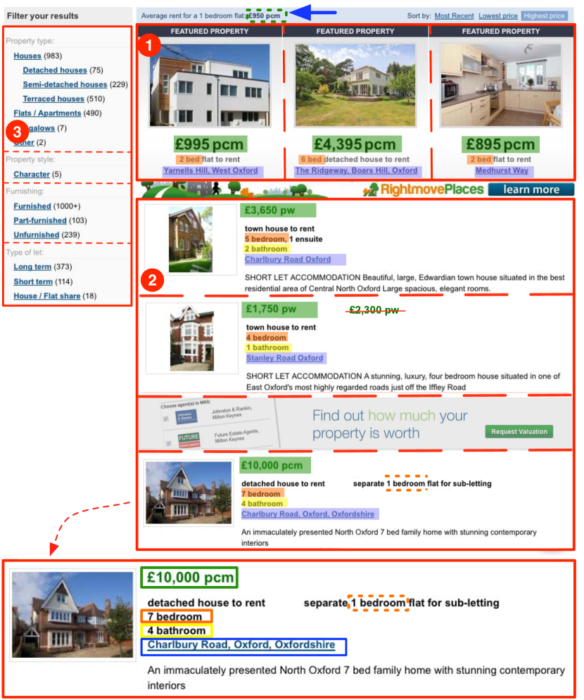
Figure 1: Result Page on rightmove.co.uk

We illustrate Amber on the result page from Rightmove, the biggest UK real estate aggregator. Figure 1 shows the typical parts of such pages: On top, (1) some featured properties are arranged in a horizontal block, while directly below, separated by an advertisement, (2) the properties matching the user’s query are listed vertically. Finally, on the left-hand side, a block (3) provides some filtering options to refine the search result. At the bottom of Figure 1 we zoom into the third record, highlighting the identified attributes.

After annotating the DOM of the page, Amber analyzes the page in three steps: data area identification, record segmentation, and attribute alignment. In all these steps we exploit annotations provided by domain-specific annotators, in particular for regular attribute types, here price, to distinguish between relevant nodes and noise such as ads.

For Figure 1, Amber identifies price annotations (highlighted in green, e.g., “£995 pcm”), most locations (purple), the number of bedrooms (orange) and bathrooms (yellow). The price on top (with the blue arrow), the “1 bedroom” in the third record, and the crossed out price in the second record are three examples of false positives annotations, which are corrected by Amber subsequently.

Data area identification.

First, Amber detects which parts of the page contain relevant data. In contrast to most other approaches, Amber deals with web pages displaying multiple, differently structured data areas. E.g., in Figure 1 Amber identifies two data areas, one for the horizontally repeated featured properties and one for the vertically repeated normal results (marked by red boxes).

Where other approaches rely solely on repeated structure, Amber first identifies pivot nodes, i.e., nodes on the page that contain annotations for regular attribute types, here price. Second, Amber obtains the data areas as clusters of continuous sequences of pivot nodes which are evenly spaced at roughly the same DOM tree depth and distance from each other. For example, Amber does not mistake the filter list (3) as a data area, despite its large size and regular structure. Approaches only analyzing structural or visual structures may fail to discard this section. Also, any annotation appearing outside the found areas is discarded, such as the price annotation with the blue arrow atop of area (1).

Record segmentation.

Second, Amber needs to segment the data area into “records”, each representing one multi-attribute object. To this end, Amber cuts off noisy pivot nodes at the head and tail of the identified sequences and removes interspersed nodes, such as the crossed out price in the second record. The remaining pivot nodes segment the data area into fragments of uniform size, each with a highly regular structure, but additional shifting may be required as the pivot node does not necessarily appear at the beginning of the record. Among the possible record segmentations the one with highest regularity among the records is chosen. In our example, Amber correctly determines the records for the data areas (1) and (2), as illustrated by the dashed lines. Amber prunes the advertisement in area (2) as inter-record noise, since it would lower the segmentation regularity.

Attribute alignment.

Finally, Amber aligns the found annotations within the repeated structure to identify the record attributes. Thereby, Amber requires that each attribute occurs in sufficiently many records at corresponding positions. If this is the case, it is well-supported, and otherwise, the annotation is dropped. Conversely, a missing attribute is inferred, if sufficiently many records feature an annotation of the same type at the position in concern. For example, all location annotations in data area $2$ share the same position, and thus need no adjustment. However, for the featured properties, the annotators may fail to recognize “Medhurst Way” as a location. Amber infers nevertheless that “Medhurst Way” must be a location (as shown in Figure 1), since all other records have a location at the corresponding position. For data area $2$, bathroom and bedroom number are shown respectively at the same relative positions. However, the third record also states that there is a separate flat to sublet with one bedroom. This node is annotated as bedroom number, but Amber recognizes it is false positive due to the lack of support from other records.

To summarise, Amber addresses low recall and precision of annotations in the attribute alignment, as it can rely on an already established record segmentation to determine the regularity of the attributes. In addition it compensates for noise in the annotations for regular attribute types in the record segmentation by majority voting to determine the length of a record and by dropping irregular annotations (such as the crossed out price in record 2). Amber also addresses noise in the regular structure on the page, such as advertisements between records and regular, but irrelevant areas on the page such as the refinement links. All this comes at the price of requiring some domain knowledge about the attributes and their instances in the domain, that can be easily acquired from just a few examples, as discussed in Section 4.

2 Multi-Attribute Object Extraction

2.1 Result Page Anatomy

Amber extracts multi-attribute objects from result pages, i.e., pages that are returned as a response to a form query on a web site. The typical anatomy of a result page is a repeated structure of more or less complex records, often in form of a simple sequence. Figure 1 shows a typical case, presenting a paginated sequence of records, each representing a real estate property to rent, with a price, a location, the number of bed and bath rooms.

We call record each instance of an object on the page and we refer to a group of continuous and similarly structured records as data area. Then, result pages for a schema $\Sigma=\Sigma_{R}\cup\Sigma_{O}$ that defines the optional and regular attribute types of a domain have the following characteristics: • Each data area consists of (D1) a maximal and (D2) continuous sequence of records,while each record (D3) is a sequence of children of the data area root, and consists of (R1) a continuous sequence of sibling subtrees in the DOM tree. For all records, this sequence is of (R2) the same length, of (R3) the same repeating structure, and contains (R4) in most cases one instance of each regular attribute in $\Sigma_{R}$. Furthermore, each record may contain (R5) instances of some optional attributes $\Sigma_{O}$, such that attributes for all attribute types in $\Sigma_{R}\cup\Sigma_{O}$ (R6) appear at similar positions within each record, if they appear at all. For attributes, we note that relevant attributes (A1) tend to appear early within their record, with (A2) its textual content filling a large part of their surrounding text box. Also (A3) attributes for optional attribute types tend to be less standardized in their values, represented with more variations.

Result pages comes in many shapes, e.g., grids, like the one depicted in Figure 2 taken from the appalachianrealty.com real estate website, tables, or even simple lists. The prevalent case, however, is the sequence of individual records as in Figure 1.

Many result pages on the web are regular, but many also contain considerable noise. In particular, an analysis must (N1) tolerate inter-record noise, such as advertisements between records, and (N2) intra-record noise, such as instances of attribute types such as price occurring also in product descriptions. It must also (N3) address pages with multiple data areas distinguish them from regular, but irrelevant noise. .

Further Examples.

Consider a typical result page from Zoopla.co.uk (Figure 3). Here we have two distinct data areas where records are laid out using different templates. Premium (i.e., sponsored) results appear in the top data area (A), while regular results appear in the bottom data area (B). A wrapper generation system must be able to cluster the two kinds of records and distinguish the different data areas. Once the two data areas have been identified, the analysis of the records does not pose particular difficulties since, within each data area, the record structure is very regular.

Another interesting case is the presence of highlighted results like in Figure 4, again taken from Rightmove.co.uk, where premium records (A) are diversified from other results (B) within the same data area. This form of highlighting can easily complicate the analysis of the page and the generation of a suitable wrapper.

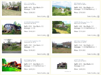
Figure 2: A grid result page.

Figure 3: Multiple data areas.

Figure 4: Premium records

2.2 Extraction Typing

For extracting multi-attribute objects, we output a data structure describing each object and its attributes, such as origin, departure time, and price. In addition, to automatically induce wrappers, Amber needs not only to extract this data but must also link the extracted data to its representation on the originating pages. To that end, Amber types nodes in the DOM for extraction (extraction typing) to describe (1) how objects appear on the page as records, (2) how attributes are structured within records, and (3) how records are grouped into data areas. In supervised wrapper induction systems, this typing is usually provided by humans “knowing” the objects and their attributes. But in fully unsupervised induction, also the generation of the extraction typing is automated. To formalise extraction typing, we first define a web page and then type its nodes according to a suitable domain schema.

Web pages.

Following Benedikt2007XPath-Leashed , we represent a web page as its DOM tree $P=\bigl{(}(U)_{U\in\textsf{unary}},{\textsf{child}},{\textsf{next-sibl}}\bigr{)}$ where each $\lambda\in(U)_{U\in\textsf{unary}}$ is a unary relation to label nodes with $\lambda$, ${\textsf{child}}(p,c)$ holds if $p$ is a parent node of $c$, and ${\textsf{next-sibl}}(s,s^{\prime})$ holds if $s^{\prime}$ is the sibling directly following $s$. In abuse of notation, we refer to $P$ also as the set of DOM nodes in $P$. Further relations, e.g., descendant and following, are derived from these basic relations. We write $x\prec y$, if $x$ is a preceding sibling of $y$, and we write $x\preceq y$ for $x\prec y$ or $x=y$. For all nodes $n$ and $n^{\prime}$, we define the sibling distance $n-_{\textsf{sibl}}n^{\prime}$ with

$$n-_{\textsf{sibl}}n^{\prime}=\left\{\begin{array}[]{lcl}n\preceq n^{\prime}&:&\hfill|\{k\mid n\prec k\preceq n^{\prime}\}|\\ n^{\prime}\prec n&:&-|\{k\mid n^{\prime}\prec k\preceq n\}|\\ \text{otherwise}&:&\infty\end{array}\right.$$

Finally, ${\textsf{first-child}}(p,c)$ holds if $c$ is the first child of $p$, i.e., if there is no other child $c^{\prime}$ of $p$ with $c^{\prime}\prec c$.

Extraction Typing.

Intuitively, data areas, records, and attributes are represented by (groups of) DOM nodes. An extraction typing formalizes this in typing the nodes accordingly to guide the induction of a suitable wrapper for pages generated from the same template and relies on a domain schema for providing attribute types. We distinguish attribute types into regular and optional, the latter indicating that attributes of that type typically occur only in some, but not all records.

Definition 1

A domain schema $\Sigma=\Sigma_{R}\cup\Sigma_{O}$ defines disjoint sets $\Sigma_{R}$ and $\Sigma_{O}$ of regular and optional attribute types.

Definition 2

Given a web page with DOM tree $P$, an extraction typing for domain schema $\Sigma=\Sigma_{R}\cup\Sigma_{O}$ is a relation $\mathcal{T}:P\times(\Sigma\cup\{\mathbf{d},\mathbf{rs},\mathbf{rt}\})$ where each node $n\in P$ with

1. $\mathcal{T}(n,\mathbf{d})$ contains a data area, with

2. $\mathcal{T}(n,\mathbf{rs})$, $n$ represents a record that spans the subtrees rooted at $n$ and its subsequent siblings $n^{\prime}$. For all these subsequent siblings $n^{\prime}$, we have

3. $\mathcal{T}(n^{\prime},\mathbf{rt})$, marking the tail of the record.

4. $\mathcal{T}(n,\rho)$ holds, if $n$ contains an attribute of type $\rho\in\Sigma$.

Data areas may not be nested, neither may records, but records must be children of a data area, and attributes must be descendants of a (single) record.

Definition 3

Given an extraction typing $\mathcal{T}$, a node $n$ is part of a record $r$, written ${\textsf{partOf}}_{\mathcal{T}}(n,r)$, if the following conditions hold: $\mathcal{T}(r,\mathbf{rs})$holds, $n$occurs in a subtree rooted at node $r^{\prime}$ with $\mathcal{T}(r^{\prime},\mathbf{rs})$ or $\mathcal{T}(r^{\prime},\mathbf{rt})$, and there is no node $r^{\prime\prime}$ between $r$ and $r^{\prime}$ with $\mathcal{T}(r^{\prime\prime},\mathbf{rs})$. A record $r$ is part of a data area $d$, written ${\textsf{partOf}}_{\mathcal{T}}(r,d)$, if $r$ is a child of $d$, and transitively, we have ${\textsf{partOf}}_{\mathcal{T}}(n,d)$ for ${\textsf{partOf}}_{\mathcal{T}}(n,r)$ and ${\textsf{partOf}}_{\mathcal{T}}(r,d)$.

Figure 5: Amber workflow

3 The AMBER Approach

Following the result page anatomy from the preceding section, the extraction of multi-attribute objects involves three main tasks: (1) Identifying data areaswith relevant objects among other noisy contents, such as advertisements or navigation menus, (2) segmentingsuch data areas into records, i.e., representations of individual objects, and (3) aligning attributesto objects, such that all records within the same data area feature a similar attribute structure.

An attempt to exploit properties (D1-3), (R1-6), and (A1-3) directly, leads to a circular search: Data areas are groups of regularly structured records, while records are data area fragments that exhibit structural similarities with all other records in the same area. Likewise, records and attributes are recognized in mutual reference to each other. Worse, automatically identifying attribute values is a naturally noisy process based on named entity recognition (e.g., for locations) or regular expressions (e.g., for postcodes or prices). Hence, to break these cyclic dependencies, we draw some basic consequences from the above characterization. Intuitively, these properties ensure that the instances of each regular attribute $\rho\in\Sigma_{R}$ constitute a cluster in each data area, • where each instance occurs (D4) roughly at the same depth in the DOM tree and (D5) roughly at the same distance.

Capitalizing on these properties, and observing that it is usually quite easy to identify the regular attributes $\Sigma_{R}$ for specific application domains, Amber relies on occurrences of those regular attributes to determine the records on a page: Given an annotator for a single such attribute $\pi\in\Sigma_{R}$ (called pivot attribute type), Amber fully automatically identifies relevant data areas and segments them into records. Taking advantage of the repeating record structure, this works well, even with fairly low quality annotators, as demonstrated in Section 6. For attribute alignment, Amber requires corresponding annotators for the other domain types, also working with low quality annotations. For the sake of simplicity, we ran Amber with a single pivot attribute per domain – achieving strong results on our evaluation domains (UK real estate and used car markets). However, one can run Amber in a loop to analyze each page consecutively with different pivot attributes to choose the extraction instance which covers most attributes on the page.

Once, a pivot attribute type has been chosen, Amber identifies and segments data areas based on pivot nodes, i.e., DOM nodes containing instances of the pivot attribute: Data areas are DOM fragments containing a cluster of pivot nodes satisfying (D4) and (D5), and records are fragments of data areas containing pivot nodes in similar positions. Once data areas and records are fixed, we refine the attributes identified so far by aligning them across different records and adding references to the domain schema. With this approach, Amber deals incomplete and noisy annotator (see Section 4), created with little effort, but still extracts multi-attribute objects without significant overhead, as compared to single attribute extraction.

Moreover, Amber deals successfully with the noise occurring on pages, i.e., it (N1) tolerates inter-record noise by recognizing the relevant data via annotations, (N2) tolerates intra-record variances by segmenting records driven by regular attributes, and it (N3) address multi-template pages by considering each data area separately for record segmentation.

3.1 Algorithm Overview

The main algorithm of Amber, shown in Algorithm 1 and Figure 5, takes as inputs a DOM tree $P$ and a schema $\Sigma=\Sigma_{R}\cup\Sigma_{O}$, with a regular attribute type $\pi\in\Sigma_{R}$ marked as pivot attribute type, to produce an extraction typing $\mathcal{T}$. First, the annotations ann for the DOM $P$ are computed as described in Section 3.2 (Line 1). Then, the extraction typing $\mathcal{T}$ is constructed in three steps, by identifying and adding the data areas (Line 1), then segmenting and adding the records (Line 1), and finally aligning and adding the attributes (Line 1). All three steps are discussed in Sections 3.3 to 3.5. Each step takes as input the DOM $P$ and the incrementally expanded extraction typing $\mathcal{T}$. The data area identification takes as further input the pivot attribute type $\pi$ (but not the entire schema $\Sigma$), together with the annotations ann. It produces – aside the data areas in $\mathcal{T}$ – the sets $\textsf{{pivots}}(d)$ of pivot nodes supporting the found data areas $d$. The record segmentation requires these pivots to determine the record boundaries to be added to $\mathcal{T}$, working independently from $\Sigma$. Only the attribute alignment needs the schema $\Sigma$ to type the DOM nodes accordingly. At last, deviances between the extraction typing $\mathcal{T}$ and the original annotations ann are exploited in improving the gazetteers (Line 1) – discussed in Section 4.

1

input : $P$ – DOM to be analyzed

input : $\Sigma=\Sigma_{R}\cup\Sigma_{O}$ – schema for the searched results, with a specifically marked pivot attribute $\pi\in\Sigma_{R}$

output : $\mathcal{T}$ – extraction typing on $P$

2

3annotate $(P,\Sigma,\textsf{ann})$;

4 identify $(P,\mathcal{T},\pi,\textsf{ann},\textsf{{pivots}})$;

5 segment $(P,\mathcal{T},\textsf{{pivots}})$;

6 align $(P,\mathcal{T},\Sigma)$;

7 learn ($\mathcal{T}$,ann);

8

Algorithm 1 $\texttt{amber}(P,\mathcal{T},\Sigma)$

3.2 Annotation Model

During its first processing step, Amber annotates a given input DOM to mark instances of the attribute types occurring in $\Sigma=\Sigma_{R}\cup\Sigma_{O}$. We define these annotations with a relation $\textsf{ann}:\Sigma\times N\times U$, where $N$ is the DOM node set, and $U$ is the union of the domains of all attribute types in $\Sigma$. $\textsf{ann}(A,n,v)$ holds, if $n$ is a text node containing a representation of a value $v$ of attribute type $A$. For the HTML fragment <span>Oxford,$\pounds$2k</span>, we obtain, e.g., $\textsf{ann}(\textsf{{location}},t,\textrm{``Oxford''})$ and $\textsf{ann}(\textsf{{price}},t,\textrm{``2000''})$, where $t$ is the text node within the span.

In Amber, we implement ann with GATE, relying on a mixture of manually crafted and automatically extracted gazetteers, taken from sources such as DBPedia Auer07dbpedia:a , along with regular expressions for prices, postcodes, etc. In Section 6, we show that Amber easily compensates even for very low quality annotators, thus requiring only little effort in creating these annotators.

3.3 Data Area Identification

We overcome the mutual dependency of data area, record, and attribute in approximating the regular record through instances of the pivot attribute type $\pi$: For each record, we aim to identify a single pivot node containing that record attribute $\pi$ (R4). A data area is then a cluster of pivot nodes appearing regularly, i.e., the nodes occur have roughly the same depth (D4) and a pairwise similar distance (D5).

Let $N_{\pi}$ be a set of pivot nodes, i.e., for each $n\in N_{\pi}$ there is some $v$ such that $\textsf{ann}(\pi,n,v)$ holds. Then we turn properties (D4) and (D5) into two corresponding regularity measures for $N_{\pi}$: • $N_{\pi}$is (M4) $\Theta^{\textsf{depth}}$-depth consistent,if there exists a $k$ such that ${\textsf{depth}}(n)=k\pm\Theta^{\textsf{depth}}$ for all $n\in N_{\pi}$, and $N_{\pi}$ is (M5) $\Theta^{\textsf{dist}}$-distance consistent,if there exists a $k$ such that $|\textsf{path}(n,n^{\prime})|=k\pm\Theta^{\textsf{dist}}$ for all $n\neq n^{\prime}\in N_{\pi}$. Therein, ${\textsf{depth}}(n)$ denotes the depth of $n$ in the DOM tree, and $|\textsf{path}(n,n^{\prime})|$ denotes the length of the undirected path from $n$ to $n^{\prime}$. Assuming some parametrization $\Theta^{\textsf{depth}}$ and $\Theta^{\textsf{dist}}$, we derive our definition of data areas from these measures:

Definition 4

A data area (for a regular attribute type $\pi$) is a maximal subtree $d$ in a DOM $P$ where

1. $d$ contains a set of pivot nodes $N_{\pi}$ with $|N_{\pi}|\geq 2$,

2. $N_{\pi}$ is depth and distance consistent (M4-5),

3. $N_{\pi}$ is maximal (D1) and continuous (D2), and

4. $d$ is rooted at the least common ancestor of $N_{\pi}$.

1

input : $P$ – DOM to be analyzed

output : $\mathcal{T}$ – extraction typing on $P$ with data areas only

input : $\pi$ – the pivot attribute type $\pi\in\Sigma_{R}$

input : ann – annoations on $P$

output : pivots – data areas support

2

3$\textsf{{pivots}}(n)\leftarrow\emptyset$ for all $n\in P$;

4 $\textnormal{{CandDAs}}\leftarrow\{\;\;(\{n\},[{\textsf{depth}}(n),{\textsf{depth}}(n)],[\infty,0])\;\;\mid\;\;\textsf{ann}(\pi,n,v)\}$;

5 $\textnormal{{CandDAs}}.add(\emptyset,[0,\infty],[0,\infty])$;

6 $\textnormal{{LastDA}}=(\textnormal{{Nodes}}_{\textnormal{{LastDA}}},\textnormal{{Depth}}_{\textnormal{{LastDA}}},\textnormal{{Dist}}_{\textnormal{{LastDA}}})\leftarrow(\emptyset,[],[])$;

7 foreach $(\textnormal{{Nodes}},\textnormal{{Depth}},\textnormal{{Dist}})\in\textnormal{{CandDAs}}$ in document order do

8       $\textnormal{{Depth}}^{\prime}\leftarrow\textnormal{{Depth}}_{\textnormal{{LastDA}}}\uplus\textnormal{{Depth}}$;

9       $\textnormal{{Dist}}^{\prime}\leftarrow\textnormal{{Dist}}_{\textnormal{{LastDA}}}\uplus\textnormal{{Dist}}\uplus\textnormal{{pathLengths}}(\textnormal{{Nodes}}_{\textnormal{{LastDA}}},\textnormal{{Nodes}})$;

10       if $|\textnormal{{Depth}}^{\prime}|<\Theta^{\textsf{depth}}$ and $|\textnormal{{Dist}}^{\prime}|<\Theta^{\textsf{dist}}$ then

             /* Cluster can be extended further */

11             $\textnormal{{LastDA}}\leftarrow(\textnormal{{Nodes}}_{\textnormal{{LastDA}}}\cup\textnormal{{Nodes}},\textnormal{{Depth}}^{\prime},\textnormal{{Dist}}^{\prime})$;

12            

13      else

             /* Cluster cannot be extended further */

14             if $|\textnormal{{Nodes}}_{\textnormal{{LastDA}}}|\geq 2$ then

15                   $d\leftarrow\textnormal{{lca}}(\textnormal{{Nodes}}_{\textnormal{{LastDA}}})$;

16                   if $|\textsf{{pivots}}(d)|<|\textnormal{{Nodes}}_{\textnormal{{LastDA}}}|$ then

17                         $\textsf{{pivots}}(d)\leftarrow\textnormal{{Nodes}}_{\textnormal{{LastDA}}}$; add $\mathcal{T}(d,\mathbf{d})$;

18                        

19                  

20            $\textnormal{{LastDA}}\leftarrow(\textnormal{{Nodes}},\textnormal{{Depth}},\textnormal{{Dist}})$;

21            

22      

Algorithm 2 $\texttt{identify}(P,\mathcal{T},\pi,\textsf{ann},\textsf{{pivots}})$

Algorithm 2 shows Amber’s approach to identifying data areas accordingly. The algorithm takes as input a DOM tree $P$, an annotation relation ann, and a pivot attribute type $\pi$. As a result, the algorithm marks all data area roots $n\in P$ in adding $\mathcal{T}(n,\mathbf{d})$ to the extraction typing $\mathcal{T}$. In addition, the algorithm computes the support of each data area, i.e., the set of pivot nodes giving rise to a data area. The algorithm assigns this support set to $\textsf{{pivots}}(n)$, for use by the the subsequent record segmentation.

The algorithm clusters pivot nodes in the document, recording for each cluster the depth and distance interval of all nodes encountered so far. Let $I=[i_{1},i_{2}]$ and $J=[j_{1},j_{2}]$ be two such intervals. Then we define the merge of $I$ and $J$, $I\uplus J=[\min(i_{1},j_{1}),\max(i_{2},j_{2})]$. A (candidate) cluster is given as tuple $(\textnormal{{Nodes}},\textnormal{{Depth}},\textnormal{{Dist}})$ where Nodes is the clustered pivot node set, and Depth and Dist are the minimal intervals over $\mathbb{N}_{0}$, such that ${\textsf{depth}}(n)\in\textnormal{{Depth}}$ and $|\textsf{path}(n,n^{\prime})|\in\textnormal{{Dist}}$ holds for all $n,n^{\prime}\in\textnormal{{Nodes}}$.

During initialization, the algorithm resets the support $\textsf{{pivots}}(n)$ for all nodes $n\in P$ (Line 2), turns all pivot nodes into a candidate data areas of size 1 (Line 2), and adds a special candidate data area $(\emptyset,[0,\infty],[0,\infty])$ (Line 2) to ensure proper termination of the algorithm’s main loop. This data area is processed after all other data areas and hence forces the algorithm in its last iteration into the else branch of Line 2 (explained below). Before starting the main loop, the algorithm initializes $\textnormal{{LastDA}}=(\textnormal{{Nodes}}_{\textnormal{{LastDA}}},\textnormal{{Depth}}_{\textnormal{{LastDA}}},\textnormal{{Dist}}_{\textnormal{{LastDA}}})$ to hold the data area constructed in the last iteration. This data area is initially empty and set to $(\emptyset,[],[])$ (Line 2).

After initialization, the algorithm iterates in document order over all candidate data areas $(\textnormal{{Nodes}},\textnormal{{Depth}},\textnormal{{Dist}})$ in CandDAs (Line 2). In each iteration, the algorithm tries to merge this data area with the one constructed up until the last iteration, i.e., with LastDA. If no further merge is possible, the resulting data area is added as a result (if some further property holds). To check whether a merge is possible, the algorithm first merges the depth and distance intervals (Lines 2 and 2, respectively). The latter is computed by merging the intervals from the clusters with a third one, pathLengths, the interval covering the path lengths between pairs of nodes from the different clusters (Line 2). If the new cluster is still $\Theta^{\textsf{depth}}$-depth and $\Theta^{\textsf{dist}}$-distance consistent (Lines 2), we merge the current candidate data area into LastDA and continue (Line 2).

Otherwise, the cluster LastDA cannot be grown further. Then, if LastDA contains at least 2 nodes (Line 2), we compute the representative $d$ of LastDA as the least common ancestor $\textnormal{{lca}}(\textnormal{{Nodes}}_{\textnormal{{LastDA}}})$ of the contained pivot nodes $\textnormal{{Nodes}}_{\textnormal{{LastDA}}}$ (Line 2). If this representative $d$ is not already bound to another (earlier occurring) support set of at least of the same size (Line 2), we assign $\textnormal{{Nodes}}_{\textnormal{{LastDA}}}$ as new support to $\textsf{{pivots}}(d)$ and mark $d$ as dataarea by adding $\mathcal{T}(d,\mathbf{d})$ (Line 2). At last, we start a to build a data area with the current one $(\textnormal{{Nodes}},\textnormal{{Depth}},\textnormal{{Dist}})$. The algorithm always enters this else branch during its last iteration to ensure that the very last data area’s pivot nodes are properly considered as a possible support set.

Theorem 3.1

The set of data areas for a DOM $P$ of size $n$ under schema $\Sigma$ and pivot attribute type $\pi$ is computed in $O(n^{2})$.

Proof

Lines 2–2 iterate twice over the DOM and are therefore in $O(n)$. Lines 2–2 are in $O(n^{2})$, as the loop is dominated by the computation of the distance intervals. For the distance intervals, we extend the interval by the maximum and minimum path length between nodes from $\textnormal{{Nodes}}_{\textnormal{{LastDA}}}$ and Nodes and thus compare any pair of nodes at most once (when merging it to the previous cluster).∎

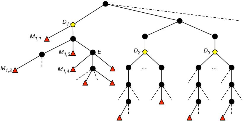
Figure 6: Data area identification

To illustrate Algorithm 2, consider Figure 6 with $\Theta^{\textsf{dist}}=\Theta^{\textsf{depth}}=3$. Yellow diamonds represent the data areas $D_{1},D_{2}$, and $D_{3}$, and red triangles pivot nodes. With this large thresholds the algorithm creates one cluster at $D_{1}$ with $M_{1,1}$ to $M_{1,4}$ as support, despite the homogeneity of the subtree rooted at $E$ and the “loss” of the three rightmost pivot nodes in $E$. In Section 6, we show that the best results are obtained with smaller thresholds, viz. $\Theta^{\textsf{dist}}=2$ and $\Theta^{\textsf{depth}}=1$, which indeed would split $D_{1}$ in this case. Also note, that $D_{2}$ and $D_{3}$ are not distance consistent and thus cannot be merged. Small variations in depth and distance, however, such as in $D_{2}$ do not affect the data area identification.

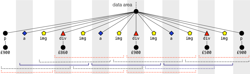
Figure 7: Record Segmentation

3.4 Record Segmentation

During the data area identification, Amber identifies data areas of a page, marks their roots $d$ with $\mathcal{T}(d,\mathbf{d})$, and provides the pivot nodes $\textsf{{pivots}}(d)$ supporting the data area, with its pivot nodes occurring roughly at the same depth and mutual distance. As in data area identification, Amber approximates the occurrence of relevant data and structural record similarity through instances of regular attribute types $\Sigma_{R}$ (R4) to construct a set of candidate segmentations. Hence, only the records in these candidate segmentations must be checked for mutual structural similarity (R3), allowing Amber to scale to large and complex pages at ease.

Definition 5

A record is a set $r$ of continuous children of a data area $d$ (R1), such that $r$ contains at least one pivot node from $\textsf{{pivots}}(d)$ (R4). A record segmentation of $d$ is a set of non-overlapping records $\mathcal{R}$ of uniform size (R2). The quality of a segmentation $\mathcal{R}$ improves with increasing size (D1) and decreasing irregularity (R3).

Given a data area root $d$ and its pivot nodes $\textsf{{pivots}}(d)$, this leads to a dual objective optimization problem, striving for a maximal area of minimal irregularity. We concretize this problem with the notion of leading nodes: Given a pivot node $n\in\textsf{{pivots}}(d)$, we call the child $l$ of $d$, containing $n$ as a descendant, the leading node $l$ of $n$. Accordingly, we define $\textsf{{leadings}}(d)$ as the set of leading nodes of a data area rooted at $d$. To measure the number of siblings of $l$ potentially forming a record, we compute the leading space $\textnormal{{lspace}}(l,L)$ after a leading node $l\in L$ as the sibling distance $l-_{\textsf{sibl}}l^{\prime}$, where $l^{\prime}\in L$ is the next leading node in document order. The two objectives for finding an optimal record segmentation $\mathcal{R}$ are then as follows:

1. Maximize the subset $\mathcal{R}^{\prime}\subseteq\mathcal{R}$ of records that are evenly segmented (D1). A subset $\mathcal{R}^{\prime}=\{r_{1},\dots r_{k}\}$ is evenly segmented if each record $r_{i}\in\mathcal{R}^{\prime}$ contains exactly one pivot node $n_{i}\in\textsf{{pivots}}(d)$ (R4), and all leading nodes $l_{i}$ corresponding to a pivot node $n_{i}$ have the same leading space $\textnormal{{lspace}}(l_{i},\textsf{{leadings}}(d))$ (R1-3).

2. Minimize the irregularity of the record segmentation (R3). The irregularity of a record segmentation $\mathcal{R}$ equals the summed relative tree edit distances between all pairs of nodes in different records in $\mathcal{R}$, i.e., ${\textsf{irregularity}}(\mathcal{R})=\sum_{n\in r,n^{\prime}\in r^{\prime}\text{with }r\neq r^{\prime}\in\mathcal{R}}{\textsf{editDist}}(n,n^{\prime})$, where ${\textsf{editDist}}(n,n^{\prime})$ is the standard tree edit distance normalized by the size of the subtrees rooted at $n$ and $n^{\prime}$ (their “maximum” edit distance).

Amber approximates such a record segmentation with Algorithm 3. It takes as input a DOM $P$, a data area root $d\in P$, and accesses the corresponding support sets via $\textsf{{pivots}}(d)$, as constructed by the data area identification algorithm of the preceding section. The segmentation is computed in two steps, first searching a basic record segmentation that contains a large sequence of evenly segmented pivot nodes, and second, shifting the segmentation boundaries back and forth to minimize the irregularity. In a preprocessing step all children of the data area without text or attributes (“empty” nodes) are collapsed and excluded from the further discussion, assuming that these act as separator nodes, such as br nodes.

So, the algorithm initially determines the sequence $\mathcal{L}$ of leading nodes underlying the segmentation (Line 3). Based on these leading nodes, the algorithm estimates the distance Len between leading nodes (Line 3) that yields the largest evenly segmented sequence: We take for Len the shortest leading space $\textnormal{{lspace}}(l)$ among those leading spaces occurring most often in $\mathcal{L}$. Then we deal with noise prefixes in removing those leading nodes $l_{k}$ from the beginning of $\mathcal{L}$ which have $\textnormal{{lspace}}(l_{k})$ smaller than Len (Line 3-3). After dealing with the prefixes, we drop all leading nodes from $\mathcal{L}$ whose sibling distance to the previous leading node is less than Len (Lines 3-3). This loop ensures that each remaining leading node has a leading space of at least Len and takes care of noise suffixes.

With the leading nodes $\mathcal{L}$ as a frame for segmenting the records, the algorithm generates all segmentations with record size Len such that each record contains at least one leading node from $\mathcal{L}$. To that end, the algorithm computes all possible sets StartCandidates of record start points for these records by shifting the original leading nodes $\mathcal{L}$ to the left (Line 3). The optimal segmentation $\mathcal{R}_{opt}$ is set to the empty set, assuming that the empty set has high irregularity (Line 3). We then iterate over all such start point sets $S$ (Line 3) and compute the actual segmentations $\mathcal{R}$ as the records of Len length, each starting from one starting point in $S$ (Line 3). By construction, these are records, as they are continuous siblings and contain at least one leading node (and hence at least one pivot node). The whole Segmentation is a record segmentation as its records are non-overlapping (because of Line 3-3) and of uniform size Len (Line 3). From all constructed segmentations, we choose the one with the lowest irregularity (Lines 3-3). At last, we iterate through all records $r$ in the optimal segmentation $\mathcal{R}_{opt}$ (Line 3), and mark the first node $n\in r$ as record start with $\mathcal{T}(n,\mathbf{rs})$ (Line 3) and all remaining nodes $n\in r$ as record tail with $\mathcal{T}(n,\mathbf{rt})$ (Line 3-3).

1

input : $P$ – DOM to be analyzed

input : $\mathcal{T}$ – extraction typing on $P$

input : pivots – data areas support

modifies : $\mathcal{T}$ – adds record segmentations

2

3foreach $d\in P:\mathcal{T}(d,\mathbf{d})$ do

4       $\mathcal{L}\leftarrow\textsf{{leadings}}(d)$;

5       $\textnormal{{Len}}\leftarrow\min\{\textnormal{{lspace}}(l,\mathcal{L})$: $l\in\mathcal{L}$ with maximal $|\{l^{\prime}\in\mathcal{L}:\textnormal{{lspace}}(l,\mathcal{L})=\textnormal{{lspace}}(l^{\prime},\mathcal{L})\}|\}$;

6      

7      while $l_{k}\in\mathcal{L}$ in document order, $\textnormal{{lspace}}(l_{k},\mathcal{L})<\textnormal{{Len}}$ do

8             delete $l_{k}$ from $\mathcal{L}$;

9            

10      for $l_{k}\in\mathcal{L}$ in document order do

11             if $\textnormal{{lspace}}(l_{k},\mathcal{L})<\textnormal{{Len}}$ then  delete-skip $l_{k+1}$ from $\mathcal{L}$;

12             ;

13            

14      $\textnormal{{StartCandidates}}\leftarrow\{\{n:\exists l\in\mathcal{L}:n-_{\textsf{sibl}}l=i\}:0\leq i<\textnormal{{Len}}\}$;

15       $\mathcal{R}_{opt}\leftarrow\emptyset$;

16       foreach $S\in\textnormal{{StartCandidates}}$ do

17             $\mathcal{R}=\{\{n:s-_{\textsf{sibl}}n\leq\textnormal{{Len}}\}\;:\;s\in S\}$;

18             if $\forall r\in\mathcal{R}:|r|=\textnormal{{Len}}$ then

19                   if ${\textsf{irregularity}}(\mathcal{R})<{\textsf{irregularity}}(\mathcal{R}_{opt})$ then

20                         $\mathcal{R}_{opt}\leftarrow\mathcal{R}$;

21                        

22                  

23            

24      foreach $r\in\mathcal{R}_{opt}$ do

25             foreach Node $n_{i}\in r$ in document order do

26                   add $\mathcal{T}(n_{i},\mathbf{rt})$;

27                  

28            add $\mathcal{T}(n_{1},\mathbf{rs})$;

29            

30      

Algorithm 3 segment $(P,\mathcal{T},\textsf{{pivots}}$)

Theorem 3.2

Algorithm 3 runs in $O(b\cdot n^{3})$ on a data area $d$ with $b$ as degree of $d$ and $n$ as size of the subtree below $d$.

Proof

Lines 3-3 are in $O(b^{2})$. Line 3 generates in StartCandidates at most $b$ segmentations (as $\textsf{Len}\leq b$) of at most $b$ size. The loop in Lines 3-3 is executed once for each segmentation $S\in\textnormal{{StartCandidates}}$ and is dominated by the computation of ${\textsf{irregularity}}()$ which is bounded by $O(n^{3})$ using a standard tree edit distance algorithm. Since $b\leq n$, the overall bound is $O(b^{2}+b\cdot n^{3}=b\cdot n^{3})$.∎

In the example of Figure 7, Amber generates five segmentations with $\textsf{Len}=4$, because of the three (red) div nodes, occurring at distance 4. Note, how the first and last leading nodes (p elements) are eliminated (in Lines 3-3) as they are too close to other leading nodes. Of the five segmentations (shown at the bottom of Figure 7), the first and the last are discarded in Line 3, as they contain records of a length other than $4$. The middle three segmentations are proper record segmentations, and the middle one (solid line) is selected by Amber, because it has the lowest irregularity among those three.

3.5 Attribute Alignment

After segmenting the data area into records, Amber aligns the contained attributes to complete the extraction instance. We limit our discussion to single valued attributes, i.e., attribute types which occur at most once in each record. In contrast to other data extraction approaches, Amber does not need to refine records during attribute alignment, since the repeating structure of attributes is already established in the extraction typing. It remains to align all attributes with sufficient cross-record support, thereby inferring missing attributes, eliminating noise ones, and breaking ties where an attribute occurs more than once in a single record.

When aligning attributes, Amber must compare the position of attribute occurrences in different records to detect repeated structures (R3) and to select those attribute instances which occur at similar relative positions within the records (R6). To encode the position of an attribute relative to a record, we use the path from the record node to the attribute:

Definition 6

For DOM nodes $r$ and $n$ with ${\textsf{descendant}}(r,n)$, we define the characteristic tag path $\textsf{tag-path}_{r}(n)$ as the sequence of HTML tags occurring on the path from $r$ to $n$, including those of $r$ and $n$ itself, taking only first-child and next-sibl steps while skipping all text nodes. With the exception of $r$’s tag, all HTML tags are annotated by the step type.

For example, in Figure 8, the characteristic tag path from the leftmost a and to its i descendant node is a/first-child::p/first-child::span/next-sibl::i. Based on characteristic tag paths, Amber quantifies the assumption that a node $n$ is an attribute of type $\rho\in\Sigma$ within record $r$ with support $\textsf{supp}_{\mathcal{T}}(r,n,\rho)$.

Definition 7

Let $\mathcal{T}$ be an extraction typing on DOM $P$ with nodes $d,r,n\in P$ where $n$ belongs to record $r$, and $r$ belongs to the data area rooted at $d$. Then the support $\textsf{supp}_{\mathcal{T}}(r,n,\rho)$ for $n$ as attribute instance of type $\rho\in\Sigma$ is defined as the fraction of records $r^{\prime}$ in $d$ that contain a node $n^{\prime}$ with $\textsf{tag-path}_{r}(n)=$ $\textsf{tag-path}_{r^{\prime}}(n^{\prime})$ and $\mathcal{T}(n^{\prime},\rho)$ for arbitrary $v$.

Consider a data area with 10 records, containing 1 price-annotated node $n_{1}$ with tag path div/…/next-sibl::span within record $r_{1}$, and 3 price-annotated nodes $n_{2}\dots n_{4}$ with tag path div/…/first-child::p within records $r_{2}\dots r_{4}$, resp. Then, $\textsf{supp}_{\mathcal{T}}(r_{1},n_{1},\textsf{{price}})=0.1$ and $\textsf{supp}_{\mathcal{T}}(r_{i},n_{i},\textsf{{price}})=0.3$ for $2\leq i\leq 4$.

With the notion of support at hand, we define our criterion for an acceptable extraction typing $\mathcal{T}$ – which we use to transform incomplete and noise annotations into consistent attributes: We turn annotations into attributes if the support is strong enough, and with even stronger support, we also infer attributes without underlying annotation.

Definition 8

An extraction typing $\mathcal{T}$ over schema $\Sigma=\Sigma_{R}\cup\Sigma_{O}$ and DOM $P$ is well-supported, if for all nodes $n$ with $\mathcal{T}(n,\rho)$, one of the following two conditions is satisfied – setting $X=R$ for $\rho\in\Sigma_{R}$ and $X=O$ for $\rho\in\Sigma_{O}$: (1) $\textsf{supp}_{\mathcal{T}}(r,n,\rho)>\Theta^{\textsf{infer}}_{X}$, or (2) $\textsf{supp}_{\mathcal{T}}(r,n,\rho)>\Theta^{\textsf{keep}}_{X}$and $\textsf{ann}(\rho,n,v)$.

This definition introduces two pairs thresholds, $\Theta^{\textsf{infer}}_{R}$, $\Theta^{\textsf{keep}}_{R}$ and $\Theta^{\textsf{infer}}_{O}$, $\Theta^{\textsf{keep}}_{O}$, respectively, for dealing with regular and optional attribute types. In both cases, we require $\Theta^{\textsf{infer}}_{X}>\Theta^{\textsf{keep}}_{X}$, as inferring an attribute without an annotation requires more support than keeping a given one. We also assume that $\Theta^{\textsf{infer}}_{R}\geq\Theta^{\textsf{infer}}_{O}$, i.e., that optional attributes are easier inferred, since optional attributes tend to come with more variations (creating false negatives) (A3). Symmetrically, we assume $\Theta^{\textsf{keep}}_{O}\geq\Theta^{\textsf{keep}}_{R}$, i.e., that optional attributes are easier dropped, optional attributes that are not cover by the template (R5) might occur in free-text descriptions (creating false positives). Taken together, we obtain $\Theta^{\textsf{infer}}_{R}\geq\Theta^{\textsf{infer}}_{O}\geq\Theta^{\textsf{keep}}_{O}\geq\Theta^{\textsf{keep}}_{R}$. See Section 6 for details on how we set these four thresholds.

We also apply a simple pruning technique prioritizing early occurrences of attributes (A1), as many records start with some semi-structured attributes, followed by a free-text description. Thus earlier occurrences are more likely to be structured attributes rather than occurrences in product descriptions. As shown in Section 6, this simple heuristic suffices for high-accuracy attribute alignment. For clarity and space reasons, we therefore do not discuss more sophisticated attribute alignment techniques.

1

input : $P$ – DOM to be analyzed

input : $\mathcal{T}$ – extraction typing on $P$

input : $\Sigma=\Sigma_{R}\cup\Sigma_{O}$ – schema of the searched results

modifies : $\mathcal{T}$ – adds attributes

2

3foreach $\rho$ in $\Sigma$ do

4       select $X$ with $\rho\in\Sigma_{X}:$ $\Theta^{\textsf{infer}}\leftarrow\Theta^{\textsf{infer}}_{X}$; $\Theta^{\textsf{keep}}\leftarrow\Theta^{\textsf{keep}}_{X}$;

5       foreach $n,r\in P$ with ${\textsf{partOf}}_{\mathcal{T}}(n,r)$ do

6             if $\textsf{supp}_{\mathcal{T}}(r,n,\rho)>\Theta^{\textsf{infer}}$ or $\big{(}\textsf{ann}(\rho,n,v)$ and $\textsf{supp}_{E}(r,n,\rho)>\Theta^{\textsf{keep}}\big{)}$ then  add $\mathcal{T}(n,\rho)$;

7             ;

8            

9      foreach $n$ with $\rho\in\mathcal{T}(n)$ do

10             if $\exists n^{\prime}:$ $\mathcal{T}(n^{\prime},\rho)$ and ${\textsf{following}}(n^{\prime},n)$ then

11                   remove $\mathcal{T}(n,\rho)$;

12                  

13            

14      

Algorithm 4 align $(P,\mathcal{T},\Sigma)$

Algorithm 4 shows the full attribute alignment algorithm and presents a direct implementation of the well-supportedness requirement. The algorithm iterates over all attributes in the schema $\rho\in\Sigma=\Sigma_{R}\cup\Sigma_{O}$ (Line 4) and selects the thresholds $\Theta^{\textsf{infer}}$ and $\Theta^{\textsf{keep}}$ depending on whether $\rho$ is regular or optional (Line 4). Next, we iterate over all nodes $n$ which are part of a record $r$ (Line 4). We assign the attribute type $\rho$ to $n$, if the support $\textsf{supp}_{\mathcal{T}}(r,n,\rho)$ for $n$ having type $\rho$ is reaching either the inference threshold $\Theta^{\textsf{infer}}$ or the keep threshold $\Theta^{\textsf{keep}}$, requiring additionally an annotation $\textsf{ann}(\rho,n,v)$ in the latter case (Line 4). After finding all nodes $n$ with enough support to be typed with $\rho$, we remove all such type assignments except for the first one (Lines 4-4).

Theorem 3.3

Amber’s attribute alignment (Algorithm 4) computes a well-supported extraction instance for a page with DOM $P$ in $O(|\Sigma|\cdot|P|)$.

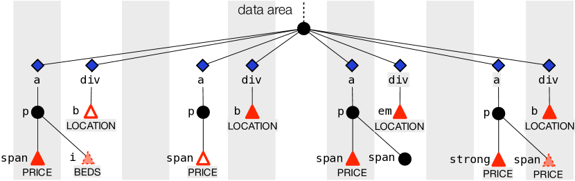
Figure 8: Attribute alignment

In Figure 8 we illustrate attribute alignment in Amber for $\Theta^{\textsf{infer}}=40\%$ for both regular and optional attribute types and $\Theta^{\textsf{keep}}_{R}=0\%$, $\Theta^{\textsf{keep}}_{O}=30\%$ (price and location regular, beds optional): The data area has four records each spanning two of the children of the data area (shown as blue diamonds). Red triangles represent attributes with the attribute type written below. Other labels are HTML tags. A filled triangle is an attribute directly derived from an annotation, an empty triangle one inferred by the algorithm in Line $6$. In this example, the second record has no price annotation. However, there is a span with tag path a/first-child::p/first-child::span and there are two other records (the first and third) with a span with the same tag path from their record. Therefore that span has support $>\Theta^{\textsf{infer}}=40\%$ for price and is added as a price attribute to the second record. Similarly, for the b element in record $1$ we infer type location from the support in record $2$ and $4$. Record $3$ has a location annotation, but in an em. This has only $25\%$ support, but since location is regular that suffices. This contrasts to the i in record $1$ which is annotated as beds and is not accepted as an attribute since optional attributes need at least $\Theta^{\textsf{keep}}_{O}=30\%$ support. In record $4$ the second price annotation is ignored since it is the second in document order (Lines 7–8).

3.6 Running Example

Recall Figure 1 in Section 1.1, showing the web page of rightmove.co.uk, an UK real estate aggregator, which we use as running example: It shows a typical result page with one data area with featured properties (1), a second area with regular search results (2), and a menu offering some filtering options (3).

For this web page, Figure 9 shows a simplified DOM along with the raw annotations for the attribute types price, bedRoomNumber, and location, as provided by our annotation engine (for simplicity, we do not consider the bathRoomNumber shown on the original web page). Aside the very left nodes in Figure 9, belonging to the filter menu, the DOM consists of a single large subtree with annotated data. The numbered red arrows mark noise or missing annotations – to be fixed by Amber: (1) This node contains indeed a price, but outside any record: It is the average rent over the found results, occurring at the very top of Figure 1. (2) The location annotation in the third record is missing. (3) The second price in this record is shown crossed out, and is therefore noise to be ignored. (4) This bedroom number refers to a flat to sublet within a larger property and is therefore noise.

Data Area Identification.

For identifying the data areas, shown in Figure 10, Algorithm 2 searches for instances of the pivot attribute type – price in this case. Amber clusters all pivot nodes which are depth and distance consistent for $\Theta^{\textsf{depth}}=\Theta^{\textsf{dist}}=1$ into one data area, obtaining the shown Areas 1 and 2. The price instance to the very left (issue (1) named above) does not become part of a cluster, as it its distance to all other occurrences is 6, whereas the occurrence inside the two clusters have mutual distance 4, with $4+\Theta^{\textsf{dist}}<6$. For same reason, the two clusters are not merged, as the distance between one node from Area 1 and one from Area 2 is also 6. The data area is then identified by the least common ancestor of the supporting pivot nodes, called the data area root.

Record Segmentation.

The record segmentation in Algorithm 3 processes each data areas in isolation: For a given area, it first determines the leading nodes corresponding to the pivot nodes, shown as solid black nodes in Figure 10. The leading node of a pivot node is the child of the data area root which is on the path from the area root to the pivot node. In case of Area 1 to the left, all children of the area root are leading nodes, and hence, each subtree rooted at a leading nodes becomes a record in its own right, producing the segmentation shown to the left of Figure 11. The situation within Area 2 is more complicated: Amber first determines the record length to be 2 sibling children of the area root, since in most cases, the leading nodes occur in a distance of 2, as shown in Figure 10. Having fixed the record length to 2, Amber drops the leading nodes which follow another leading node too closely, eliminating the leading node corresponding to the noisy price in the second record (issue (3) from above). Once the record length and the resulting leading nodes are fixed, Algorithm 3 shifts the records boundaries to find the right segmentation, yielding two alternatives, shown on the right of Figure 11. In the upper variant, only the second and fourth record are similar, the first and third record deviate significantly, causing a lot of irregularity. Hence, the lower variant is selected, as its four records have a similar structure.

Attribute Alignment.

Algorithm 4 fixes the attributes of the records, leading to the record structure shown in lower half of Figure 12. This infers the missing location and cleans the noisy price (issues (2) and (4) from above). One the upper left of Figure 12, we show the characteristic tag path for location is computed, resulting in a support of $2/3$, as we have 2 location occurrences at the same path within 3 records – with e.g. $\Theta^{\textsf{infer}}_{O}=50\%$ enough to infer the location attribute without original annotation. On the upper right of Figure 12, we show how the noisy price in the third record is eliminating: Again, the characteristic tag paths are shown, leading to a support of $1/4$ – with e.g. $\Theta^{\textsf{keep}}_{O}=30\%$ too low to keep the bedRoomNumber attribute. The resulting data area and record layout is shown in the bottom of Figure 12.

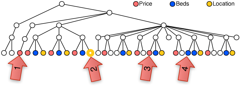
Figure 9: Simplified DOM for rightmove.co.uk

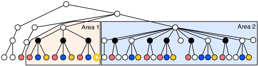
Figure 10: Data area identification on rightmove.co.uk

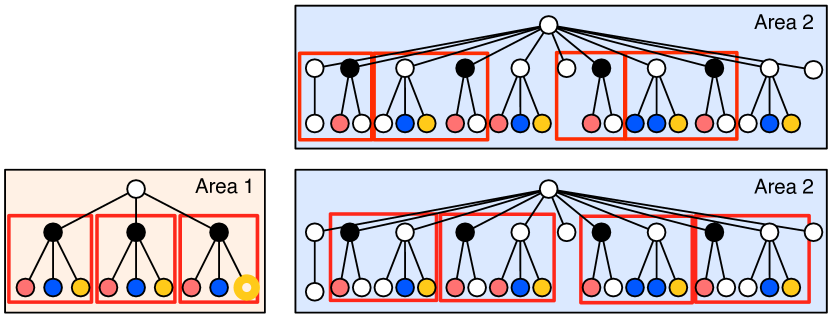
Figure 11: Record Segmentation on rightmove.co.uk

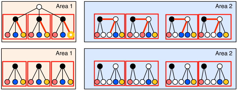
Figure 12: Attribute Alignment on rightmove.co.uk

4 Building the Domain Knowledge

In Amber we assume that the domain schema is provided upfront by the developer of the wrapper. In particular, for a given extraction task, the developer must specify only the schema $\Sigma=\Sigma_{R}\cup\Sigma_{O}$ of regular and optional attribute types, using the regular attribute types as strong indicators for the presence of a $\Sigma$ entity on a webpage. In addition, the developer can also specify disjointness constraints $\rho_{1}\wedge\rho_{2}\rightarrow\bot$ for two attribute types $\rho_{1},\rho_{2}\in\Sigma$ to force the domains of $\rho_{1}$ and $\rho_{2}$ to be disjoint.

As mentioned earlier, devising basic gazetteers and regular expressions for core entities of a given domain requires very little work thanks to frameworks like GATE Cun11 and openly available knowledge repositories such as DBPedia Auer07dbpedia:a and FreeBase Bollacker08 . Values that can be recognised with regular expressions are usually known a priori, as they correspond to common-sense entities, e.g., phone numbers or monetary values. On the other hand, the construction of gazetteers, i.e., sets of terms corresponding to the domains for attribute types (see Section 2), is generally a tedious task. While it is easy to construct an initial set of terms for an attribute type, building a complete gazetteer often requires an exhaustive analysis of a large sample of relevant web pages. Moreover, the domains of some attribute types are constantly changing, for example a gazetteer for song titles is outdated quite quickly. Hence, in the following, we focus on the automatic construction and maintenance of gazetteers and show how Amber’s repeated-structure analysis can be employed for growing small initial term sets into complete gazetteers.

This automation lowers the need and cost for domain experts in the construction of the necessary domain knowledge, since even a non-expert can produce basic gazetteers for a domain to be completed by our automated learning processes. Moreover, the efficient construction of exhaustive gazetteers is valuable for other applications outside web data extraction, e.g., to improve existing annotation tools or to publish them as linked open data for public use.

But even if a gazetteer is curated by a human, the resulting annotations might still be noisy due to errors or intrinsic ambiguity in the meaning of the terms. Noise-tolerance is therefore of paramount importance in repairing or discarding wrong examples, given enough evidence to support the correction. To this end, Amber uses the repeated structure analysis to infer missing annotations and to discard noisy ones, incrementally growing small seed lists of terms into complete gazetteers, and proving that sound and complete initial domain knowledge is, in the end, unnecessary.

1

input : $\mathcal{T}$ – extraction typing for $P$

input : ann – annotations for $P$

input : $\mathcal{U}=\{U_{1},\ldots,U_{k}\}$ – domains of the attribute types

modifies : $\mathcal{U}$ – modifies domains of attribute types

2 foreach $\left<n,\rho\right>\in\mathcal{T}$ do

3       Terms $\leftarrow$ components ($n$);

4       foreach $v\in\textnormal{{Terms}}\ |\ v\not\in\overline{U}_{\rho}$ do

5             if $\left<\rho,n,v\right>\not\in\textsf{ann}$ then

6                   add $v$ to $U_{\rho}$;

7                   $\textnormal{{ev}}(v,U_{\rho})\leftarrow\textnormal{{ev}}(v,\overline{U}_{\rho})\leftarrow 0$;

8                  

9            $\textnormal{{ev}}(v,U_{\rho})\leftarrow\textnormal{{ev}}(v,U_{\rho})+\textnormal{{freq}}^{+}(v,\rho,\mathcal{T})$;

10            

11      

12foreach $\textsf{ann}(\rho,n,v)|\left<n,\rho\right>\not\in\mathcal{T}$ do

13       $\textnormal{{ev}}(v,\overline{U}_{\rho})\leftarrow\textnormal{{ev}}(v,\overline{U}_{\rho})+\textnormal{{freq}}^{-}(v,\rho,\mathcal{T})$;

14       if $\textnormal{{ev}}(v,U_{\rho})<\Theta\cdot\textnormal{{ev}}(v,\overline{U}_{\rho})$ then

15             add $v$ to $\overline{U}_{\rho}$;

16            

17      

Algorithm 5 learn $(\mathcal{T},\textsf{ann},\mathcal{U}$)

Learning in Amber can be carried in two different modes: (1) In upfront learning, Amber produces upfront domain knowledge for a domain to bootstrap the self-supervised wrapper generation. (2) In continuous learning, Amber refines the domain knowledge over time, as Amber extracts more pages from websites of a given domain of previously unknown terms from nodes selected within the inferred repeated structure. Regardless the learning mode, the core principle behind Amber’s learning capabilities is the mutual reinforcement of repeated-structure analysis and the automatic annotation of the DOM of a page.

For the sake of explanation, a single step of the learning process is described in Algorithm 5. To update the gazetteers in $\mathcal{U}=\{U_{1},\ldots,U_{k}\}$ from an extraction typing $\mathcal{T}$ and the corresponding annotations ann, for each node $n$, we compare the attribute types of $n$ in $\mathcal{T}$ with the annotations ann for $n$. This comparison leads to three cases:

1. Term validation: $n$ is a node attribute for $\rho$ and carries an annotation $\textsf{ann}(\rho,n,v)$. Therefore, $v$ was part of the gazetteer for $\rho$ and the repeated-structure analysis confirmed that $v$ is in the domain $U_{\rho}$ of the attribute type.

2. Term extraction: $n$ is a node attribute for $\rho$ but it does not carry an annotation $\textsf{ann}(\rho,n,v)$. Therefore, Amber should consider the terms in the textual content of $n$ for adding to the domain $U_{\rho}$.

3. Term cleaning: The node carries an annotation $\textsf{ann}(\rho,n,v)$ but does not correspond to an attribute node for $\rho$ in $\mathcal{T}$, i.e., is noise for $\rho$. Therefore, Amber must consider whether there is enough evidence to keep $v$ in $U_{\rho}$.

For each attribute node $n$ in the extraction typing $\mathcal{T}$, Amber applies the function components to tokenize the textual content of the attribute node $n$ to remove unwanted token types (e.g., punctuation, separator characters, etc.) and to produce a clean set of tokens that are likely to represent terms from the domain. For example, assume that the textual content of a node $n$ is the string $w$=“Oxford, Walton Street, ground-floor apartment”. The application of the function components produces the set $\langle$ “Oxford”, “Walton Street”, “ground-floor”, “apartment”$\rangle$ by removing the commas from $w$.

Amber then iterates over all terms that are not already known to occur in the complement $\overline{U}_{\rho}$ of the domain of the attribute type $\rho$ and decides whether it is necessary to validate or add them to the set of known values for $\rho$. A term $v$ is in $\overline{U}_{\rho}$ if is either known from the schema that $v\in U_{\rho^{\prime}}$ and $\Sigma\models\rho\wedge\rho^{\prime}\rightarrow\bot$, or $v$ has been recurrently identified by the repeated-structure analysis as noise. Each term $v$ has therefore an associated value $\textsf{ev}(v,U_{\rho})$ (resp. $\textsf{ev}(v,\overline{U}_{\rho})$) representing the evidence of $v$ appearing — over multiple learning steps — as a value for $\rho$ (resp. as noise for $\rho$).

If Amber determined that a node $n$ is an attribute node of type $\rho$ but no corresponding annotation $\textsf{ann}(\rho,n,v)$ exists, then we add them to the domain $U_{\rho}$. Moreover, once the term $v$ is known to belong to $U_{\rho}$ we simply increase its evidence by a factor $\textsf{freq}^{+}(v,\rho,\mathcal{T})$ that represent how frequently $v$ appeared as a value of $\rho$ in the current extraction typing $\mathcal{T}$. The algorithm then proceeds to the reduction of the noise in the gazetteer by checking those cases where an annotation $\textsf{ann}(\rho,n,v)$ is not associated to any attribute node in the extraction typing, i.e., it is noise for $\rho$. Every time a term $v$ is identified as noise we increase the value of $\textsf{ev}(v,\overline{U}_{\rho})$ of a factor $\textsf{freq}^{-}(v,\rho,\mathcal{T})$ that represents how frequently the term $v$ occur as noise in the current typing $\mathcal{T}$. To avoid the accumulation of noise, Amber will permanently add a term $v$ to $\overline{U}_{\rho}$ if the evidence that $v$ is noisy for $\rho$ is at least $\Theta$ times larger that the evidence that $v$ is a genuine value for $\rho$. The constant $\Theta$ is currently set to 1.5.

Figure 13: Amber Learning Interface

To make the construction of the gazetteers even smoother, Amber also provides a graphical facility (see Figure 13) that enables developers to understand and possibly drive the learning process. Amber’s visual component provides a live graphical representation of the result of the repeated-structure analysis on individual pages and the position of the attributes (1). Amber relates the concepts of the domain schema (3), e.g., location and property-type, with (3) the discovered terms, providing also the corresponding confidence value. The learning process is based on the analysis of a selected number of pages from a list of URLs (4). The terms that have been identified on the current page and have been validated are added to the gazetteer (5).

5 System Architecture

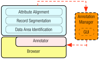
Figure 14: System architecture

Figure 14 shows Amber’s architecture composed of mainly of three layers. The Browser Layer consists of a JAVA API that abstracts the specific browser implementation actually employed. Through this API, currently Amber supports a real browser like Mozilla Firefox, as well as a headless browser emulator like HTMLUnit. Amber uses the browser to retrieve the web page to analyze, thus having direct access to its DOM structure. Such DOM tree is handed over to the Annotator Layer. This is implemented such that different annotators can be plugged in and used in combination, regardless their actual nature, e.g., web-service or custom standalone application. Given an annotation schema for the domain at hand, such layer produces annotations on the input DOM tree using all registered annotators. Further, the produced annotations are reconciliated w.r.t. constraints present in the annotation schema. Currently, annotations in Amber are performed by using a simple GATE (gate.ac.uk) pipeline consisting of gazetteers of terms and transducers (JAPE rules). Gazetters for real estate and used cars domains are either manually-collect (for the most part) or derived from external sources such as DBPedia and Freebase. Note that many types are common across domains (e.g., price, location, date), and that the annotator layer allows for arbitrary entity recognisers or annotators to be integrated.

With the annotated DOM at hand, Amber can begin its analysis with data area identification, record segmentation and attribute alignments. Each of these phases is a distinct sub-module, and all of them are implemented in Datalog rules on top of a logical representation of the DOM and its annotations. These rules are with finite domains and non-recursive aggregation, and executed by the engine DLV.

As described in Section 3, the outcome of this analyses is an extraction typing $\mathcal{T}$ along with attributes and relative support. During Amber’s bootstrapping, however, $\mathcal{T}$ is in turn used as feedback to realize the learning phase (see Sect. 4, managed by the Annotation Manager module. Here, positive and negative lists of candidate terms is kept per each type, and used to update the initial gazetteers lists. The Annotation Manager is optionally complemented with a graphical user interface, implemented as an Eclipse plugin (eclipse.org) which embeds the browser for visualization.

6 Evaluation

Amber is implemented as a three-layer analysis engine where (1) the web access layer embeds a real browser to access and interact with the live DOM of web pages, (2) the annotation layer uses GATE Cun11 along with domain gazetteers to produce annotations, and (3) the reasoning layer implements the actual Amber algorithm as outlined in Section 3 in datalog rules over finite domains with non-recursive aggregation.

6.1 AMBER in the UK

We evaluate Amber on $150$ UK real-estate web sites, randomly selected among $2\,810$ web sites named in the yellow pages, and $100$ UK used car dealer websites, randomly selected from UK’s largest used car aggregator autotrader.co.uk. To assure diversity in our corpus, in case two sites use the same template, we delete one of them and randomly choose another one. For each site, we obtain one, or if possible, two result pages with at least two result records. These pages form the gold standard corpus, that is manually annotated for comparison with Amber. For the UK real estate, the corpus contains $281$ pages with $2\,785$ records and $14\,614$ attributes. The used car corpus contains $151$ pages with $1\,608$ records and $12\,732$ attributes.

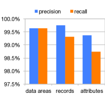
(a) Real Estate

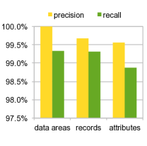
(b) Used Cars

Figure 15: Evaluation Overview

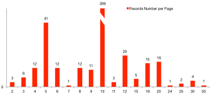
Figure 16: Distribution of Records Per Page

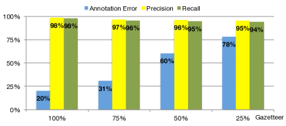
Figure 17: Amber Robustness wrt. Noise in Gazetteers

For the following evaluations we use threshold values as $\Theta^{\textsf{depth}}=1$, $\Theta^{\textsf{dist}}=2$ and $\Theta^{\textsf{infer}}_{R}=\Theta^{\textsf{infer}}_{O}=50\%$, $\Theta^{\textsf{keep}}_{R}=0\%$, and $\Theta^{\textsf{keep}}_{O}=20\%$. Figures 15a and 15b show the overall precision and recall of Amber on the real estate and used car corpora. As usual, precision is defined as the fraction of recognized data areas, records, or attributes that are also present in the gold standard, whereas recall as the fraction of all data areas, records, and attributes in the gold standard that is returned by Amber. Amber achieves outstanding precision and recall on both domains ($>98\%$). If we measure the average precision and recall per site (rather than the total precision and recall), pages with fewer records have a higher impact. But even in that harder case, precision and recall remains above $97.5\%$.

Robustness.

More importantly, Amber is very robust both w.r.t. noise in the annotations/structure and w.r.t. the number of repeated records per page. To give an idea, in our corpus $50\%$ of pages contain structural noise either in the beginning or in the final part of the data area. Also, $70\%$ of the pages contain noisy annotations for the price attribute, that is used as regular attribute in our evaluation. On average, we count about 22 false occurrences per page. Nonetheless, Amber is able to perform nearly perfect accuracy, fixing noise both from structure and annotations. Even worse, $100\%$ of pages contain noise for the Location (i.e., addresses/locality, no postcode) attribute, which on average amounts to more than 50 (false positive) annotations of this type per page. To demonstrate how Amber copes with noisy annotations, we show in Figure 17 the correlation between the noise levels (i.e., errors and incompleteness in the annotations) and Amber’s performance in the extraction of the location attribute. Even by using the full list of locations, about $20\%$ of all annotations are missed by the annotators, yet Amber achieves $>98\%$ precision and recall. If we restrict the list to $75\%,50\%$, and finally just $25\%$ of the original list, the error rate rises over $30\%$ and $60\%$ to $78\%$. Nevertheless, Amber’s accuracy remains nearly unaffected dropping by only $3\%$ to about $95\%$ (measuring here, of course, only the accuracy of extraction location attributes). In other words, despite only getting annotations for one out of every five locations, Amber in able to infer the other locations from the regular structure of the records. Amber remains robust even if we introduce errors for more than one attribute, as long as there is one regular attribute such as the price for which the annotation quality is reasonable. This distinguishes Amber from all other approaches based on automatic annotations that require reasonable quality (or at least, reasonable recall). Amber, achieves high performance even from very poor quality annotators that can be created with low effort.

At the same time, Amber is very robust w.r.t. the number of records per page. Figure 16 illustrates the distribution of record numbers per page in our corpora. They mainly range from 4 to 20 records per page, with peaks for 5 and 10 records. Amber performs well on both small and large pages. Indeed, even in the case of only 3 records, it is able to exploit the repeated structure to achieve the correct extraction.

Distance, depth, and attribute alignment thresholds can influence the performance of Amber. However, it is straightforward to choose good default values for these. For instance, considering the depth and distance thresholds, Figure 22 shows that the pair ($\Theta^{\textsf{depth}}=1$,$\Theta^{\textsf{dist}}=2$) provides significantly better performance than ($0$,$0$) or ($2$,$4$).

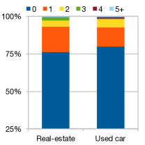
(a) Accuracy per Type

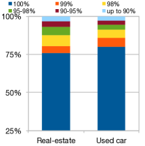
(b) Accuracy per Number

Figure 18: Attribute Extraction

Attributes.

As far as attributes are concerned, there are $9$ different types for the real estate domain, and $12$ different types for the used car corpus. First of all, in $96\%$ of cases Amber perfectly recognizes objects, i.e., properly assigns all the attributes to the belonging object. It mistakes one attribute in $2\%$ of cases, and 2 and 3 attributes only in $1\%$ of cases, respectively.

Figure 19 illustrates the precision and recall that Amber achieves on each individual attribute type of the real estate domain, where Amber reports nearly perfect recall and very high precision ($>96\%$). The results in the used car domain are similar (Figure 20) except for location, where Amber scores $91.3\%$ precision. The reason is that, in this particular domain, car models have a large variety of acronyms which happen to coincide with British postcodes, $e.g.$, N5 is the postcode of Highbury, London, X5 is a model of BMW, that also appear with regularity on the pages.

Figures 18 shows that on the vast majority of pages Amber achieves near perfect accuracy. Notably, in $97\%$ of cases, Amber retrieves correctly between $90\%$ and $100\%$ of the attributes. The percentage of cases in which Amber identifies attributes from all attribute types is above 75%, while only one type of attribute is wrong in $17\%$ of the pages. For the remaining $6\%$ of pages Amber misidentifies attributes from $2$ or $3$ types, with only one page in our corpora on which Amber fails for $4$ attribute types. This emphasizes that on the vast majority of pages at best one or two attribute types are problematic for Amber (usually due to inconsistent representations or optionality).

Figure 19: Real Estate Attributes Evaluation

Figure 20: Used Car Attributes Evaluation

6.2 Large-Scale Evaluation.

To demonstrate Amber’s ability to deal with a large set of diverse sites, we perform an automated experiment beyond the sites catalogued in our gold standard. In addition to the $150$ sites in our real estate gold standard, we randomly selected another $350$ sites from the $2\,810$ sites named in the yellow pages. On each site, we manually perform a search until we reach the first result page and retrieve all subsequent $n$ result pages and the expected number of result records on the first $n-1$ pages, by manually counting the records on the first page and assuming that the number of records remains constant on the first $n-1$ pages (on the $n$th page the number might be smaller). This yields $2\,215$ result pages overall with an expected number of $20\,723$ results records. On this dataset, Amber identifies $20\,172$ records. Since a manual annotation is infeasible at this scale, we compare the frequencies of the individual types of the extracted attributes with the frequencies of occurrences in the gold standard, as shown in Figure 21. Assuming that both dataset are fairly representative selections of the whole set of result pages from the UK real-estate domain, the frequencies of attributes should mostly coincide, as is the case in Figure 21. Indeed, as shown in Figure 21 price, location, and details page deviate by less than $2\%$, legal status, bathroom, and reception number by less than $5\%$. The high correlation strongly suggests that the attributes are mostly identified correctly. Postcode and property type cause a higher deviations of $18\%$ and $12\%$, respectively. They are indeed attributes that are less reliably identified by Amber, due to the reason explained above for UK postcodes and due to the property type often appearing only within the free text property description.

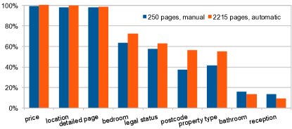
Figure 21: Attribute Frequencies in Large Scale Extraction

6.3 Comparison with other Tools

Comparison with RoadRunner.

We evaluate Amber against RoadRunner crescenzi02:_roadr , a fully automatic system for web data extraction. RoadRunner does not extract data areas and records explicitly, therefore we only compare the extracted attributes. RoadRunner attempts to identify all repeated occurrences of variable data (“slots” of the underlying page template) and therefore extracts too many attributes. For example, RoadRunner extracts on some pages more than $300$ attributes, mostly URLs and elements in menu structures, where our gold standard contains only $90$ actual attributes. To avoid biasing the evaluation against RoadRunner, we filter the output of RoadRunner, by removing the description block, duplicate URLs, and attributes not contained in the gold standard, such as page or telephone numbers.

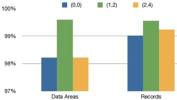
Figure 22: Depth/Distance Thresholds ($\Theta^{\textsf{depth}}$,$\Theta^{\textsf{dist}}$)

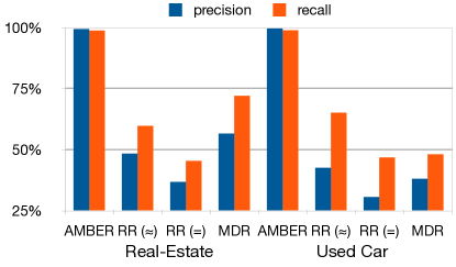
Figure 23: Comparison with RoadRunner and MDR

Another issue in comparing Amber with RoadRunner is that RoadRunner only extracts entire text nodes. For example, RoadRunner might extract “Price £114,995”, while Amber would produce “£114,995”. Therefore we evaluate RoadRunner in two ways, once counting an attribute as correctly extracted if the gold standard value is contained in one of the attributes extracted by RoadRunner (RR $\approx$ in Figure 23), and once counting an attribute only as correctly extracted if the strings exactly match (RR $=$ in Figure 23). Finally, as RoadRunner works better with more than one result page from the same site, we exclude sites with a single result page from this comparison. The results are shown in Figure 23. Amber outperforms RoadRunner by a wide margin, which reaches only $49\%$ in precision and $66\%$ in recall compared to almost perfect scores for Amber. As expected, recall is higher than precision in RoadRunner.

Comparison with MDR.

We further evaluate Amber with MDR, an automatic system for mining data records in web pages. MDR is able to recognize data areas and records, but unlike Amber, not attributes. Therefore in our comparison we only consider precision and recall for data areas and records in both real estate and used cars domains. Also for the comparison with RoadRunner, we avoid biasing the evaluation against MDR filtering out page portions e.g., menu, footer, pagination links, whose regularity in structure misleads MDR. Indeed, these are recognized by MDR as data areas or records. Figure 23 illustrates the results. In all cases, Amber outperforms MDR which on used-cars reports $57\%$ in precision and $72\%$ in recall as best performance. MDR suffers the complex structure of data records, which may contain optional information as nested repeated structure. This, in turn, are often (wrongly) recognized by MDR as record (data area).

6.4 AMBER Learning

The evaluation of Amber’s learning capabilities is done with respect to the upfront learning mode discussed in Section 4. In particular, we want to evaluate Amber’s ability of constructing an accurate and complete gazetteer for an attribute type from an incomplete and noisy seed gazetteer. We show that at each learning iteration (see Algorithm 5 in Section 4) the accuracy of the gazetteer is significantly improved, and that the learning process converges to a stable gazetteer after few iterations, even in the case of attribute types with large and/or irregular value distributions in their domains.

Setting.

In the evaluation that follows we show Amber’s learning behaviour on the location attribute type. In our setting, the term location refers to formal geographical locations such as towns, counties and regions, e.g., “Oxford”, “Hampshire”, and “Midlands”. Also, it is often the case that the value for an attribute type consists of multiple and somehow structured terms, e.g., “The Old Barn, St. Thomas Street - Oxford”. The choice of location as target for the evaluation is justified by the fact that this attribute type has typically a very large domain consisting of ambiguous and severely irregular terms. Even in the case of UK locations alone, nearly all terms from the English vocabulary either directly correspond to a location name (e.g., “Van” is a location in Wales) or they are part of it (e.g., “Barnwood”, in Gloucestershire). The ground truth for the experiment consists of a clean gazetteer of 2010 UK locations and 1,560 different terms collected from a sample of 235 web pages sourced from 150 different UK real-estate websites.

Execution.

We execute the experiment on two different seed gazetteers $G_{20}$ (resp. $G_{25}$) consisting of a random sample of 402 (resp. 502) UK locations corresponding to the $20\%$ (resp. $25\%$) of the ground truth.

Table 1: Learning performance on $G_{20}$.

rnd.	LE	CE	PE	RE	LL	CL
1	1009	763	75.65%	37.96%	169	147
2	1300	1063	81.77%	52.89%	222	196
3	1526	1396	91.48%	69.45%	224	205
4	1845	1773	96.10%	88.21%	59	52
5	1862	1794	96.35%	89.25%	23	19
6	1862	1794	96.35%	89.25%	0	0

By taking as input $G_{20}$, the learning process saturates (i.e., no new terms are learned or dropped) after six iterations with a $92.66\%$ accuracy (F₁-score), while with $G_{25}$, only 5 iterations are needed for an accuracy of $92.79\%$. Note that at the first iteration the accuracy is $50.54\%$ for $G_{20}$ and $60.94\%$ for $G_{25}$ Table 1 and Table 2 show the behaviour for each learning round. We report the number of locations extracted (L^E), i.e., the number of attribute nodes carrying an annotation of type location; among these, C^E locations have been correctly extracted, leading to a precision (resp. recall) of the extraction of P^E (resp. R^E). The last two columns show the number of learned instances (L^L), i.e., those added to the gazetteer and, among these, the correct ones (C^L).

It is easy to see that the increase in accuracy is stable in all the learning rounds and that the process quickly converges to a stable gazetteer.

Table 2: Learning performance on $G_{25}$.

rnd.	LE	CE	PE	RE	LL	CL
1	1216	983	80.84%	48.91%	289	248
2	1538	1334	86.74%	66.37%	225	204
3	1717	1617	94.18%	80.45%	57	55
4	1960	1842	93.98%	91.64%	44	35
5	1960	1842	93.98%	91.64%	0	0

7 Related Work

The key assumption in web data extraction is that a large fraction of the data on the web is structured DBLP:journals/cacm/CafarellaHM11 by HTML markup and visual styling, especially when web pages are automatically generated and populated from templates and underlying information systems. This sets web data extraction apart from information extraction where entities, relations, and other information are extracted from free text (possibly from web pages).

Early web data extraction approaches address data extraction via manual wrapper development hammer97:_semis_data or through visual, semi-automated tools Baumgartner2001VisualWebIEwithLixto ; laender02:_debye (still commonly used in industry). Modern web data extraction approaches, on the other hand, overwhelmingly fall into one of two categories (for recent surveys, see chang06:_survey_of_web_infor_extrac_system ; 565137 ): Wrapper induction DBLP:conf/sigmod/DalviBS09 ; freitag00:_machin_learn_for_infor_exrtr ; DBLP:conf/icde/GulhaneMMRRSSTT11 ; hsu98:_gener_finit_state_trans_for ; JiLi10 ; DBLP:journals/dke/KosalaBBB06 ; kushmerick97:_wrapp_induc_for_infor_extrac ; muslea01:_hierar_wrapp_induc_for_semis_infor_system starts from a number of manually annotated examples, i.e., pages where the objects and attributes to be extracted are marked by a human, and automatically produce a wrapper program which extracts the corresponding content from previously unseen pages. Unsupervised wrapper generation crescenzi02:_roadr ; kayed10:_fivat ; liu06:_vision_based_web_data_recor_extrac ; simon05:_viper ; su09ode ; DBLP:conf/kdd/WangCWPBGZ09 ; zhai06:_struc_data_extrac_from_web attempts to fully automate the extraction process by unsupervised learning of repeated structures on the page as they usually indicate the presence of content to be extracted.

Unfortunately, where the former are limited in automation, the latter are in accuracy. This has caused a recent flurry of approaches DBLP:conf/vlds/CreoCQM12 ; DBLP:journals/pvldb/DalviKS11 ; DBLP:conf/icde/DerouicheCA12 ; SMM*08 that like Amber attempt to automatise the production of examples for wrapper inducers through existing entity recognisers or similar automatic annotators. Where these approaches differ most is how and to what extend they address the inevitable noise in these automatic annotations.

7.1 Wrapper Induction Approaches

Wrapper induction can deliver highly accurate results provided correct and complete input annotations. The process is based on the iterative generalization of properties (e.g., structural and visual) of the marked content on the input examples. The learning algorithms infer generic and possibly robust extraction rules in a suitable format, e.g., XPath expressions DBLP:conf/sigmod/DalviBS09 ; DBLP:conf/icde/GulhaneMMRRSSTT11 or automata hsu98:_gener_finit_state_trans_for ; muslea01:_hierar_wrapp_induc_for_semis_infor_system , that are applicable to similar pages for extracting the data they are generated from.

The structure of the required example annotations differs across different tools, impacting the complexity of the learned wrapper and the accuracy this wrapper achieves. Approaches such as freitag00:_machin_learn_for_infor_exrtr ; DBLP:journals/dke/KosalaBBB06 operate on single attribute annotations, i.e., annotations on a single attribute or multiple, but a-priori unrelated attributes. As a result, the wrapper learns the extraction rules independently for each attribute, but, in the case of multi-attribute objects, this requires a subsequent reconciliation phase. The approaches presented in hsu98:_gener_finit_state_trans_for ; kushmerick97:_wrapp_induc_for_infor_extrac ; muslea01:_hierar_wrapp_induc_for_semis_infor_system are based on annotated trees. The advantage w.r.t. single-attribute annotations is that tree annotations make easier to recognize nested structures.

By itself, wrapper induction is incapable of scaling to the web. Because of the wide variation in the template structures of given web sites, it is practically impossible to annotate a sufficiently large page set to cover all relevant combinations of features indicating the presence of structured data. More formally, the sample complexity for web-scale supervised wrapper induction is too high in all but some restricted cases, as in e.g. DBLP:conf/kdd/WangCWPBGZ09 which extracts news titles and bodies. Furthermore, traditional wrapper inducers are very sensitive to incompleteness and noise in the annotations thus requiring considerable human effort to create such low noise and complete annotations.

7.2 Unsupervised Web Data Extraction

The completely unsupervised generation of wrappers has been based on discovering regularities on pages presumably generated by a common template. Works such as  kayed10:_fivat ; liu03:_minin_data_recor_in_web_pages ; liu06:_vision_based_web_data_recor_extrac ; simon05:_viper ; zhai06:_struc_data_extrac_from_web ; zhao05:_fully_autom_wrapp_gener_for_searc_engin ; zhao06:_autom_extrac_of_dynam_recor discuss domain-independent approaches that only rely on repeated HTML markup or regularities in the visual rendering. The most common task that can be solved by these tools is record segmentation liu03:_minin_data_recor_in_web_pages ; zhao05:_fully_autom_wrapp_gener_for_searc_engin ; zhao06:_autom_extrac_of_dynam_recor , where an area of the page is segmented into regular blocks each representing an object to be extracted. Unfortunately, these systems are quite susceptible to noise in the repeated structure as well as to regular, but irrelevant structures such as navigation menus. This limits their accuracy severely, as also demonstrated in Section 6. In Amber, having domain specific annotators at hand, we also exploit the underlying repeated structure of the pages, but guided by occurrences of regular attributes which allow us to distinguish relevant data areas from noise, as well as to address noise among the records. This allows us to extract records with higher precision.

A complementary line of work deals with specifically stylized structures, such as tables DBLP:journals/pvldb/CafarellaHWWZ08 ; Gatterbauer:2007:TDI:1242572.1242583 and lists DBLP:journals/vldb/ElmeleegyMH11 . The more clearly defined characteristics of these structures enable domain-independent algorithms that achieve fairly high precision in distinguish genuine structures with relevant data from structures created only for layout purposes. They are particular attractive for use in settings such as web search that optimise for coverage over all sites rather than recall from a particular site.

Instead of limiting the structure types to be recognized, one can exploit domain knowledge to train more specific models. Domain-dependent approaches such as DBLP:conf/kdd/WangCWPBGZ09 ; ZNW*06 exploit specific properties for record detection and attribute labeling. However, besides the difficulty of choosing the features to be considered in the learning algorithm for each domain, changing the domain usually results in at least a partial retraining of the models if not an algorithmic redesign.

More recent approaches are, like Amber and the approaches discussed in Section 7.3, domain-parametric, i.e., they provide a domain-independent framework which is parameterized with a specific application domain. For instance, su09ode uses a domain ontology for data area identification but ignores it during record segmentation.

7.3 Combined Approaches

Besides Amber, we are only aware of three other approaches DBLP:journals/pvldb/DalviKS11 ; DBLP:conf/icde/DerouicheCA12 ; SMM*08 that exploit the mutual benefit of unsupervised extraction and induction from automatic annotations. All these approaches are a form of self-supervised learning, a concept well known in the machine learning community and that has already been successfully applied in the information extraction setting springerlink:10.1007/s10115-007-0110-6 .

In SMM*08 , web pages are independently annotated using background knowledge from the domain and analyzed for repeated structures with conditional random fields (CRFs). The analysis of repeated structures identifies the record structure in searching for evenly distributed annotations to validate (and eventually repair) the learned structure. Conceptually, SMM*08 differs from Amber as it initially infers a repeating page structure with the CRFs independently of the annotations. Amber, in contrast, analyses only those portions of the page that are more likely to contain useful and regular data. Focusing the analysis of repeated structures to smaller areas is critical for learning an accurate wrapper since complex pages might contain several regular structures that are not relevant for the extraction task at hand. This is also evident from the reported accuracy of the method proposed in SMM*08 that ranges between $63\%$ and $85\%$ on attributes, which is significantly lower than Amber’s accuracy.

This contrasts also with DBLP:journals/pvldb/DalviKS11 which aims at making wrapper induction robust against noisy and incomplete annotations, such that fully automatic and cheaply generated examples are sufficient. The underlying idea is to induce multiple candidate wrappers by using different subsets of the annotated input. The candidate wrappers are then ranked according to a probabilistic model, considering both features of the annotations and the page structure. This work has proven that, provided that the induction algorithm satisfies few reasonable conditions, it is possible to produce very accurate wrappers for single-attribute extraction, though sometimes at the price of hundreds of calls of the wrapper inducer. For multi-attribute extraction, DBLP:journals/pvldb/DalviKS11 reports high, if considerably lower accuracy than in the single-attribute case. More importantly, the wrapper space is considerably larger as the number of attributes acts as a multiplicative factor. Unfortunately, no performance numbers for the multi-attribute case are reported in DBLP:journals/pvldb/DalviKS11 . In contrast, Amber fully addresses the problem of multi-attribute object extraction from noisy annotations by eliminating the annotation errors during the attribute alignment. Moreover, Amber also avoids any assumptions on a subsequently employed wrapper induction system.

A more closely-related work is ObjectRunner DBLP:conf/icde/DerouicheCA12 , a tool driven by an intensional description of the objects to be extracted (a SOD in the terminology of DBLP:conf/icde/DerouicheCA12 ). A SOD is basically a schema for a nested relation with attribute types. Each type comes with associated annotators (or recognizers) for annotating the example pages to induce the actual wrapper from by a variant of ExAlg arasu03:_extrac_struc_data_from_web_pages . The SOD limits the wrapper space to be explored ($\leq$20 calls of the inducer) and improves the quality of the extracted results. This is similar to Amber, though Amber not only limits the search space, but also considers only alternative segmentations instead of full wrappers (see Section 3.4). On the other hand, the SOD can seriously limit the recall of the extraction process, in particular, since the matching conditions of a SOD strongly privilege precision. The approach is furthermore limited by the rigid coupling of attribute types to separators (i.e., token sequences acting act as boundaries between different attribute types). It fact attribute types appear quite frequently together with very diverse separators (e.g., caused by a special highlighting or by a randomly injected advertisement). The process adopted in Amber is not only tolerant to noise in the annotations but also to random garbage content between attributes and between records as it is evident from the results of our evaluation: Where ObjectRunner reports that between $65\%$ and $86\%$ of the objects in $5$ domains ($75\%$ in the car domain) are extracted without any error, Amber is able to extract over $95\%$ of the objects from the real estate and used car domain without any error.

8 Conclusion

Amber pushes the state-of-the-art in extraction of multi-attribute objects from the deep web, through a fully-automatic approach that combines the analysis of the repeated structure of the web page and automatically-produced annotations. Amber compensates for noise in both the annotations and the repeated structure to achieve $>98\%$ accuracy for multi-attribute object extraction. To do so, Amber requires a small amount of domain knowledge that can is proven (Section 4) to be easily obtainable from just a few example instances and pages.

Though Amber is outperforming existing approaches by a notable margin for multi-attribute extraction on product domains, there remain a number of open issues in Amber and multi-attribute object extraction in general:

1. Towards irregular, multi-entity domains. Domains with multiple entity types have not been a focus of data extraction systems in the past and pose a particular challenge to approaches such as Amber that are driven by domain knowledge. While dealing with the (frequent) case in which these heterogeneous objects share a common regular attribute is fairly straightforward, more effort it is necessary when regular attributes are diverse. To this end, more sophisticated regularity conditions may be necessary. Similarly, the ambiguity of instance annotators may be so significant that a stronger reliance on labels in structures such as tables is necessary.

2. Holistic Data Extraction. Though data extraction involves several tasks, historically they have always been approached in isolation. Though some approaches have considered form understanding and extraction from result pages together, a truly holistic approach that tries to reconcile information from forms, result pages, details pages for individual objects, textual descriptions, and documents or charts about these objects remains an open challenge.

3. Whole-Domain Database. Amber, as nearly all existing data extraction approaches, is focused on extracting objects from a given site. Though unsupervised approaches such as Amber can be applied to many sites, such a domain-wide extraction also requires data integration between sites and opens new opportunities for cross-validation between domains. In particular, domain-wide extraction enables automated learning not only for instances as in Amber, but also for new attributes through collecting sufficiently large sets of labels and instances to use ontology learning approaches.

9 Acknowledgements

The research leading to these results has received funding from the European Research Council under the European Community’s Seventh Framework Programme (FP7/2007–2013) / ERC grant agreement DIADEM, no. 246858. Giorgio Orsi has also been supported by the Oxford Martin School’s grant no. LC0910-019.

References

- (1) A. Arasu and H. Garcia-Molina. Extracting structured data from web pages. In Proc. of the ACM SIGMOD International Conference on Management of Data, pages 337–348, 2003.
- (2) S. Auer, C. Bizer, G. Kobilarov, J. Lehmann, and Z. Ives. DBPedia: A nucleus for a web of open data. In Proc. Int’l. Semantic Web Conf. (ISWC), pages 11–15, 2007.
- (3) R. Baumgartner, S. Flesca, and G. Gottlob. Visual web information extraction with lixto. In Proc. Int’l. Conf. on Very Large Data Bases (VLDB), pages 119–128. Morgan Kaufmann Publishers Inc., 2001.
- (4) M. Benedikt and C. Koch. XPath leashed. ACM Computing Surveys, 2007.
- (5) K. Bollacker, C. Evans, P. Paritosh, T. Sturge, and J. Taylor. Freebase: a collaboratively created graph database for structuring human knowledge. In SIGMOD ’08: Proceedings of the 2008 ACM SIGMOD international conference on Management of data, pages 1247–1250, New York, NY, USA, 2008. ACM.
- (6) M. J. Cafarella, A. Y. Halevy, and J. Madhavan. Structured data on the web. Communications of the ACM, 54(2):72–79, 2011.
- (7) M. J. Cafarella, A. Y. Halevy, D. Z. Wang, E. Wu, and Y. Zhang. Webtables: exploring the power of tables on the web. PVLDB, 1(1):538–549, 2008.
- (8) C.-H. Chang, M. Kayed, M. R. Girgis, and K. Shaalan. A Survey of Web Information Extraction Systems. IEEE Transactions on Knowledge and Data Engineering, 18(10), 2006.
- (9) R. Creo, V. Crescenzi, D. Qiu, and P. Merialdo. Minimizing the costs of the training data for learning web wrappers. In Proc. of 2nd International Workshop on Searching and Integrating New Web Data Sources, pages 35–40, 2012.
- (10) V. Crescenzi, G. Mecca, and P. Merialdo. RoadRunner: Automatic Data Extraction from Data-Intensive Web Site. In Proc. of the ACM SIGMOD International Conference on Management of Data, page 624, 2002.
- (11) H. Cunningham, D. Maynard, K. Bontcheva, V. Tablan, N. Aswani, I. Roberts, G. Gorrell, A. Funk, A. Roberts, D. Damljanovic, T. Heitz, M. A. Greenwood, H. Saggion, J. Petrak, Y. Li, and W. Peters. Text Processing with GATE (Version 6). The University of Sheffield, Department of Computer Science, 2011.
- (12) N. N. Dalvi, P. Bohannon, and F. Sha. Robust web extraction: an approach based on a probabilistic tree-edit model. In Proc. of the ACM SIGMOD International Conference on Management of Data, pages 335–348, 2009.
- (13) N. N. Dalvi, R. Kumar, and M. A. Soliman. Automatic wrappers for large scale web extraction. The Proceedings of the VLDB Endowment, 4(4):219–230, 2011.
- (14) N. Derouiche, B. Cautis, and T. Abdessalem. Automatic extraction of structured web data with domain knowledge. In Proc. International Conference on Data Engineering, pages 726–737, 2012.
- (15) H. Elmeleegy, J. Madhavan, and A. Y. Halevy. Harvesting relational tables from lists on the web. VLDB J., 20(2):209–226, 2011.
- (16) D. Freitag. Machine Learning for Information Exrtraction. Machine Learning, 39:169–202, 2000.
- (17) T. Furche, G. Gottlob, G. Grasso, G. Orsi, C. Schallhart, and C. Wang. Little Knowledge Rules The Web: Domain-Centric Result Page Extraction. In International Conference on Web Reasoning and Rule Systems (RR’11), pages 61–76, 2011.
- (18) W. Gatterbauer, P. Bohunsky, M. Herzog, B. Krüpl, and B. Pollak. Towards domain-independent information extraction from web tables. In Proceedings of the 16th international conference on World Wide Web, WWW07, pages 71–80, 2007.
- (19) P. Gulhane, A. Madaan, R. R. Mehta, J. Ramamirtham, R. Rastogi, S. Satpal, S. H. Sengamedu, A. Tengli, and C. Tiwari. Web-scale information extraction with vertex. In Proc. Int’l. Conf. on Data Engineering (ICDE), pages 1209–1220, 2011.
- (20) J. Hammer, J. McHugh, and H. Garcia-Molina. Semistructured data: the TSIMMIS experience. In Proc. East-European Symposium on Advances in Databases and Information Systems, pages 1–8, 1997.
- (21) C. Hsu and M. Dung. Generating finite-state transducers for semistructured data extraction from the web. Information Systems, 23(8):521–538, 1998.
- (22) N. Jindal and B. Liu. A generalized tree matching algorithm considering nested lists for web data extraction. In SIAM Intl Conf. on Data Mining, pages 930–941, 2010.
- (23) M. Kayed and C.-H. Chang. FiVaTech: Page-Level Web Data Extraction from Template Pages. IEEE Transactions on Knowledge and Data Engineering, 22(2):249–263, 2010.
- (24) R. Kosala, H. Blockeel, M. Bruynooghe, and J. V. den Bussche. Information extraction from structured documents using k-testable tree automaton inference. Data and Knowledge Engineering, 58(2):129–158, 2006.
- (25) N. Kushmerick, D. S. Weld, and R. Doorenbos. Wrapper Induction for Information Extraction. In Proc. Confercence on Very Large Databases, 1997.
- (26) A. H. Laender, B. Ribeiro-Nero, and A. S. da Silva. DEByE – Data Extraction by Example. Data and Knowledge Engineering, 40(2):121–154, 2002.
- (27) A. H. F. Laender, B. A. Ribeiro-Neto, A. S. da Silva, and J. S. Teixeira. A brief survey of web data extraction tools. SIGMOD Record, 31(2):84–93, 2002.
- (28) B. Liu, R. Grossman, and Y. Zhai. Mining data records in web pages. In Proc. ACM SIGKDD Confercence on Knowledge Discovery and Data Mining, pages 601–605, 2003.
- (29) W. Liu, X. Meng, and W. Meng. Vision-based Web Data Records Extraction. In Proc. International Workshop on the Web and Databases, pages 20–25, 2006.
- (30) I. Muslea, S. Minton, and C. A. Knoblock. Hierarchical Wrapper Induction for Semistructrued Information Systems. Autonomous Agents and Multi-Agent Systems, 4:93–114, 2001.
- (31) B. Rozenfeld and R. Feldman. Self-supervised relation extraction from the web. Knowledge and Information Systems, 17:17–33, 2008.
- (32) P. Senellart, A. Mittal, D. Muschick, R. Gilleron, and M. Tommasi. Automatic wrapper induction from hidden-web sources with domain knowledge. In Proc. of WIDM, pages 9–16, 2008.
- (33) K. Simon and G. Lausen. ViPER: Augmenting Automatic Information Extraction with visual Perceptions. In Proc. ACM Conference on Information and Knowledge Management, pages 381–388, 2005.
- (34) W. Su, J. Wang, and F. H. Lochovsky. ODE: Ontology-Assisted Data Extraction. ACM Transactions on Database Systems, 34(2), 2009.
- (35) J. Wang, C. Chen, C. Wang, J. Pei, J. Bu, Z. Guan, and W. V. Zhang. Can we learn a template-independent wrapper for news article extraction from a single training site? In KDD, pages 1345–1354, 2009.
- (36) Y. Zhai and B. Liu. Structured Data Extraction from the Web Based on Partial Tree Alignment. IEEE Transactions on Knowledge and Data Engineering, 18(12):1614–1628, 2006.
- (37) H. Zhao, W. Meng, Z. Wu, V. Raghavan, and C. Yu. Fully Automatic Wrapper Generation For Search Engines. In Proc. International World Wide Web Conference, pages 66–75, 2005.
- (38) H. Zhao, W. Meng, and C. Yu. Automatic Extraction of Dynamic Record Sections From Search Egine Result Pages. In Proc. Confercence on Very Large Databases, pages 989–1000, 2006.
- (39) J. Zhu, Z. Nie, J. Wen, B. Zhang, and W. Ma. Simultaneous record detection and attribute labeling in web data extraction. In Proc. ACM SIGKDD Confercence on Knowledge Discovery and Data Mining, pages 494–503, 2006.