Greedy algorithms for high-dimensional non-symmetric linear problems

Abstract

In this article, we present a family of numerical approaches to solve high-dimensional linear non-symmetric problems. The principle of these methods is to approximate a function which depends on a large number of variates by a sum of tensor product functions, each term of which is iteratively computed via a greedy algorithm [20]. There exists a good theoretical framework for these methods in the case of (linear and nonlinear) symmetric elliptic problems. However, the convergence results are not valid any more as soon as the problems considered are not symmetric. We present here a review of the main algorithms proposed in the literature to circumvent this difficulty, together with some new approaches. The theoretical convergence results and the practical implementation of these algorithms are discussed. Their behaviors are illustrated through some numerical examples.

Introduction

High-dimensional problems arise in a wide range of fields such as quantum chemistry, molecular dynamics, uncertainty quantification, polymeric fluids, finance… In all these contexts, one wishes to approximate a function $u$ depending on $d$ variates $x_{1}$, …, $x_{d}$ where $d\in{\mathbb{N}}^{*}$ is typically very large. Classically, the function $u$ is defined as the solution of a Partial Differential Equation (PDE) and cannots be obtained by standard approximation techniques such as Galerkin methods for instance. Indeed, let us consider a discretization basis with $N$ degrees of freedom for each variate ($N\in{\mathbb{N}}^{*}$), so that the discretization space is given by

$$V_{N}:=\mbox{\rm Span}\left\{\psi_{i_{1}}^{(1)}(x_{1})\cdots\psi_{i_{d}}^{(d)}(x_{d}),\;1\leq i_{1},\cdots,i_{d}\leq N\right\},$$

where for all $1\leq j\leq d$, $\left(\psi_{i}^{(j)}\right)_{1\leq i\leq N}$ is a family of $N$ functions which only depend on the variate $x_{j}$. A Galerkin method consists in representing the solution $u$ of the initial PDE as

$$u(x_{1},\cdots,x_{d})\approx\sum_{1\leq i_{1},\cdots,i_{d}\leq N}\lambda_{i_{1},\cdots,i_{d}}\psi_{i_{1}}^{(1)}(x_{1})\cdots\psi_{i_{d}}^{(d)}(x_{d}),$$

and computing the set of $N^{d}$ real numbers $\left(\lambda_{i_{1},\cdots,i_{d}}\right)_{1\leq i_{1},\cdots,i_{d}\leq N}$. Thus, the size of the finite-dimensional problem to solve grows exponentially with the number of variates involved in the problem. Such methods cannot be implemented when $d$ is too large: this is the so-called curse of dimensionality [2].

Several approaches have recently been proposed in order to circumvent this significant difficulty. Let us mention among others sparse grids [21], tensor formats [11], reduced bases [4] and adaptive polynomial approximations [6].

In this paper, we will focus on a particular kind of methods, originally introduced by Ladevèze et al. to do time-space variable separation [12], Chinesta et al. to solve high-dimensional Fokker-Planck equations in the context of kinetic models for polymers [1] and Nouy in the context of uncertainty quantification [15], under the name of Progressive Generalized Decomposition (PGD) methods.

Let us assume that each variate $x_{j}$ belongs to a subset ${\cal X}_{j}$ of ${\mathbb{R}}^{m_{j}}$, where $m_{j}\in{\mathbb{N}}^{*}$ for all $1\leq j\leq d$. For each $d$-uplet $(r^{(1)},\cdots,r^{(d)})$ of functions such that $r^{(j)}$ only depends on $x_{j}$ for all $1\leq j\leq d$, we call a tensor product function and denote by $r^{(1)}\otimes\cdots\otimes r^{(d)}$ the function which depends on all the variates $x_{1},\cdots,x_{d}$ and is defined by

$$r^{(1)}\otimes\cdots\otimes r^{(d)}:\left\{\begin{array}[]{ccc}{\cal X}_{1}\times\cdots\times{\cal X}_{d}&\to&{\mathbb{R}}\\ (x_{1},\cdots,x_{d})&\mapsto&r^{(1)}(x_{1})\cdots r^{(d)}(x_{d}).\\ \end{array}\right.$$

The approach of Ladevèze, Chinesta, Nouy and coauthors consists in approximating the function $u$ by a separate variable decomposition, i.e.

$$u(x_{1},\cdots,x_{d})\approx\sum_{k=1}^{n}r_{k}^{(1)}(x_{1})\cdots r_{k}^{(d)}(x_{d})=\sum_{k=1}^{n}r_{k}^{(1)}\otimes\cdots\otimes r_{k}^{(d)}(x_{1},\cdots,x_{d}),$$ (1)

for some $n\in{\mathbb{N}}^{*}$. In the above sum, each term is a tensor product function. Each $d$-uplet of functions $\left(r_{k}^{(1)},\cdots,r_{k}^{(d)}\right)$ is iteratively computed in a greedy [20] way: once the first $k$ terms in the sum (1) have been computed, they are fixed, and the $(k+1)^{th}$ term is obtained as the next best tensor product function to approximate the solution. This will be made precise below.

Thus, the algorithm consists in solving several low-dimensional problems whose dimensions scale linearly with the number of variates and may be implementable when classical methods are not. In this case, if we use a discretization basis with $N$ degrees of freedom per variate as above, the size of the discretized problems involved in the computation of a $d$-uplet $\left(r_{k}^{(1)},\cdots,r_{k}^{(d)}\right)$ scales like $Nd$ and the total size of the discretization problems is $nNd$.

This numerical strategy has been extensively studied for the resolution of (linear or nonlinear) elliptic problems [20, 13, 10, 5, 18]. More precisely, let $u$ be defined as the unique solution of a minimization problem of the form

$$u=\mathop{\mbox{\rm argmin}}_{v\in V}\mathcal{E}(v),$$ (2)

where $V$ is a reflexive Banach space of functions depending on the $d$ variates $x_{1}$, …, $x_{d}$, and $\mathcal{E}:V\to{\mathbb{R}}$ is a coercive real-valued energy functional. Besides, for all $1\leq j\leq d$, let $V_{x_{j}}$ be a reflexive Banach space of functions which only depend on the variate $x_{j}$. The standard greedy algorithm reads:

1. set $u_{0}=0$ and $n=1$;

2. find $\left(r_{n}^{(1)},\cdots,r_{n}^{(d)}\right)\in V_{x_{1}}\times\cdots\times V_{x_{d}}$ such that

   $$\left(r_{n}^{(1)},\cdots,r_{n}^{(d)}\right)\in\mathop{\mbox{argmin}}_{\left(r^{(1)},\cdots,r^{(d)}\right)\in V_{x_{1}}\times\cdots\times V_{x_{d}}}\mathcal{E}\left(u_{n-1}+r^{(1)}\otimes\cdots\otimes r^{(d)}\right),$$

3. set $u_{n}=u_{n-1}+r_{n}^{(1)}\otimes\cdots\otimes r_{n}^{(d)}$ and $n=n+1$.

Under some natural assumptions on the spaces $V$, $V_{x_{1}}$, …, $V_{x_{d}}$ and the energy functional $\mathcal{E}$, all the iterations of the greedy algorithm are well-defined and the sequence $(u_{n})_{n\in{\mathbb{N}}^{*}}$ strongly converges in $V$ towards the solution $u$ of the original minimization problem (2).

This result holds in particular when $u$ is defined as the unique solution of

$$\left\{\begin{array}[]{l}\mbox{\rm find }u\in V\mbox{\rm such that}\\ \forall v\in V,\;a(u,v)=l(v),\\ \end{array}\right.$$

where $V$ is a Hilbert space, $a$ a symmetric continuous coercive bilinear form on $V\times V$ and $l$ a continuous linear form on $V$. In this case, $u$ is equivalently solution of a minimization problem of the form (2) with $\mathcal{E}(v)=\frac{1}{2}a(v,v)-l(v)$ for all $v\in V$.

However, when the function $u$ cannot be defined as the solution of a minimization problem of the form (2), designing efficient iterative algorithms is not an obvious task. This situation occurs typically when $u$ is defined as the solution of a non-symmetric linear problem

$$\left\{\begin{array}[]{l}\mbox{\rm find }u\in V\mbox{\rm such that}\\ \forall v\in V,\;a(u,v)=l(v),\\ \end{array}\right.$$

where $a$ is a non-symmetric continuous bilinear form on $V\times V$ and $l$ is a continuous linear form on $V$.

The aim of this article is to give an overview of the state of the art of the numerical methods based on the greedy iterative approach used in this non-symmetric linear context and of the remaining open questions concerning this issue. In Section 1, we present the standard greedy algorithm for the resolution of symmetric coercive high-dimensional problems and the theoretical convergence results proved in this setting. Section 2 explains why a naive transposition of this algorithm for non-symmetric problems is doomed to failure and motivates the need for more subtle approaches. Section 3 describes the certified algorithms existing in the literature for non-symmetric problems. All of them consist in symmetrizing the original non-symmetric problem by minimizing the residual of the equation in a well-chosen norm. However, depending on the choice of the norm, either the conditioning of the discretized problems may behave badly or several intermediate problems may have to be solved online, which leads to a significant increase of simulation times and memory needs compared to the original algorithm in a symmetric linear coercive case. So far, there are no methods avoiding these two problems and for which there are theoretical convergence results in the general case. In Section 4, we present some existing algorithms designed by Nouy [16] and Lozinski [14] to circumvent these difficulties and the partial theoretical results which are known for these algorithms. Section 5 is concerned with another algorithm we propose, for which some partial convergence results are proved. In Section 6, the behaviors of the different algorithms presented here are illustrated on simple toy numerical examples. Lastly, we present in the Appendix some possible tracks to design other methods, but for which further work is needed.

1 The symmetric coercive case

1.1 Notation

Let us first introduce some notation. Let $d$ be a positive integer, $m_{1}$, …, $m_{d}$ positive integers and ${\cal X}_{1}$, …,${\cal X}_{d}$ open subsets of ${\mathbb{R}}^{m_{1}}$, …, ${\mathbb{R}}^{m_{d}}$ respectively.

Let $\mu_{x_{1}}$, …, $\mu_{x_{d}}$ denote measures on ${\cal X}_{1}$, …, ${\cal X}_{d}$ respectively. Let $L^{2}({\cal X}_{1};\mu_{x_{1}})$, …, $L^{2}({\cal X}_{d};\mu_{x_{d}})$ be associated $L^{2}$ spaces, i.e. vectorial spaces which are complete when endowed with the scalar products

$$\forall f,g\in L^{2}({\cal X}_{j};\mu_{x_{j}}),\quad \langle f,g\rangle_{{\cal X}_{j}}:=\int_{{\cal X}_{j}}f(x_{j})g(x_{j})\,\mu_{x_{j}}(dx_{j}),\;\forall 1\leq j\leq d,$$

and their associated norms $\|\cdot\|_{{\cal X}_{1}}$, …, $\|\cdot\|_{{\cal X}_{d}}$. For instance, in the case when ${\cal X}_{1}=(0,1)$ and $\mu_{x_{1}}$ is the standard Lebesgue measure on ${\cal X}_{1}$, the spaces $L^{2}(0,1)$, $L^{2}_{\rm per}(0,1)$ and $L^{2}_{0}(0,1):=\left\{f\in L^{2}(0,1),\;\int_{0}^{1}f=0\right\}$ are examples of such $L^{2}$ spaces.

In the rest of this article, for the sake of simplicity, we will omit the reference to the measures $\mu_{x_{1}}$, …, $\mu_{x_{d}}$ and denote by $L^{2}({\cal X}_{1})=L^{2}({\cal X}_{1};\mu_{x_{1}})$, …, $L^{2}({\cal X}_{d})=L^{2}({\cal X}_{d};\mu_{x_{d}})$.

We introduce the space $L^{2}({\cal X}_{1}\times\cdots\times{\cal X}_{d}):=L^{2}({\cal X}_{1})\otimes\cdots\otimes L^{2}({\cal X}_{d})$. This space is a Hilbert space when endowed with the natural scalar product

$$\forall f,g\in L^{2}({\cal X}_{1}\times\cdots\times{\cal X}_{d}),\quad\langle f,g\rangle:=\int_{{\cal X}_{1}\times\cdots\times{\cal X}_{d}}f(x_{1},\cdots,x_{d})g(x_{1},\cdots,x_{d})\,\mu_{x_{1}}(dx_{1})\,\cdots\mu_{x_{d}}(dx_{d}),$$

and the associated norm is denoted by $\|\cdot\|_{{\cal X}_{1}\times\cdots\times{\cal X}_{d}}$.

Let $V\subset L^{2}({\cal X}_{1}\times\cdots\times{\cal X}_{d})$, $V_{x_{1}}\subset L^{2}({\cal X}_{1})$, …, $V_{x_{d}}\subset L^{2}({\cal X}_{d})$ be Hilbert spaces endowed respectively with scalar products denoted by $\langle\cdot,\cdot\rangle_{V}$, $\langle\cdot,\cdot\rangle_{V_{x_{1}}}$, …, $\langle\cdot,\cdot\rangle_{V_{x_{d}}}$ and associated norms $\|\cdot\|_{V}$, $\|\cdot\|_{V_{x_{1}}}$, …, $\|\cdot\|_{V_{x_{d}}}$.

We define $V^{\prime}$, $V_{x_{1}}^{\prime}$, …, $V_{x_{d}}^{\prime}$ as the dual spaces of $V$, $V_{x_{1}}$, …, $V_{x_{d}}$ with respect to the $L^{2}$ scalar products $\langle\cdot,\cdot\rangle$, $\langle\cdot,\cdot\rangle_{{\cal X}_{1}}$, …, $\langle\cdot,\cdot\rangle_{{\cal X}_{d}}$. These dual spaces are endowed with their natural norms $\|\cdot\|_{V^{\prime}}$ etc.

Lastly, the Riesz operator $R_{V}:V\to V^{\prime}$ is defined by

$$\forall v,w\in V,\;\langle v,w\rangle_{V}=\langle R_{V}v,w\rangle_{V^{\prime},V}.$$

It holds in particular that $\|v\|_{V}=\|R_{V}v\|_{V^{\prime}}$. Similar operators $R_{V_{x_{1}}}$, …, $R_{V_{x_{d}}}$ are introduced for the spaces $V_{x_{1}}$, …, $V_{x_{d}}$.

For any $d$-uplet $\left(r^{(1)},\cdots,r^{(d)}\right)\in V_{x_{1}}\times\cdots\times V_{x_{d}}$, we define the tensor product function $r^{(1)}\otimes\cdots\otimes r^{(d)}$ as follows

$$r^{(1)}\otimes\cdots\otimes r^{(d)}:\left\{\begin{array}[]{ccc}{\cal X}_{1}\times\cdots\times{\cal X}_{d}&\to&{\mathbb{R}}\\ (x_{1},\cdots,x_{d})&\mapsto&r^{(1)}(x_{1})\cdots r^{(d)}(x_{d}).\\ \end{array}\right.$$

In the particular case when $d=2$, we shall denote respectively $x_{1}$, ${\cal X}_{1}$, $m_{1}$, $V_{x_{1}}$ by $x$, ${\cal X}$, $m_{x}$, $V_{x}$ and $x_{2}$, ${\cal X}_{2}$, $m_{2}$, $V_{x_{2}}$ by $t$, ${\cal T}$, $m_{t}$, $V_{t}$.

Besides, for any Banach spaces $H_{1}$, $H_{2}$, the space of bounded linear operators from $H_{1}$ to $H_{2}$ will be denoted by $\mathfrak{L}(H_{1},H_{2})$.

1.2 Theoretical results

We recall here the theoretical framework of the standard greedy algorithm in the coercive symmetric case.

Let us consider the problem

$$\left\{\begin{array}[]{l}\mbox{find }u\in V\mbox{ such that}\\ \forall v\in V,\;a(u,v)=l(v),\\ \end{array}\right.$$ (3)

where

• $a(\cdot,\cdot)$ is a symmetric, coercive continuous bilinear form on $V\times V$;

• $l$ is a continuous linear form on $V$.

Then, problem (3) is equivalent to the minimization problem

$$u=\mathop{\mbox{argmin}}_{v\in V}{\cal E}(v),$$ (4)

where

$$\forall v\in V,\;{\cal E}(v):=\frac{1}{2}a(v,v)-l(v).$$ (5)

The greedy algorithm reads:

1. let $u_{0}=0$ and $n=1$;

2. define $\left(r_{n}^{(1)},\cdots,r_{n}^{(d)}\right)\in V_{x_{1}}\times\cdots\times V_{x_{d}}$ such that

   $$\left(r_{n}^{(1)},\cdots,r_{n}^{(d)}\right)\in\mathop{\mbox{\rm argmin}}_{\left(r^{(1)},\cdots,r^{(d)}\right)\in V_{x_{1}}\times\cdots\times V_{x_{d}}}{\cal E}\left(u_{n-1}+r^{(1)}\otimes\cdots\otimes r^{(d)}\right);$$ (6)

3. define $u_{n}=u_{n-1}+r_{n}^{(1)}\otimes\cdots\otimes r_{n}^{(d)}$ and set $n=n+1$.

Let us denote by

$$\Sigma:=\left\{r^{(1)}\otimes\cdots\otimes r^{(d)},\;r^{(1)}\in V_{x_{1}},\cdots,r^{(d)}\in V_{x_{d}}\right\}$$ (7)

and make the following assumptions:

• $\overline{\mbox{\rm Span}(\Sigma)}^{V}=V$;

• $\Sigma$ is weakly closed in $V$.

These assumptions are usually satisfied in the case of classical Sobolev spaces [5].

Theorem 1.1.

Assume that (A1) and (A2) are satisfied. Then, for all $n\in{\mathbb{N}}^{*}$, there exists at least one solution $\left(r^{(1)}_{n},\cdots,r_{n}^{(d)}\right)\in V_{x_{1}}\times\cdots\times V_{x_{d}}$ (not necessarily unique) to (6) and any solution satisfies $r^{(1)}_{n}\otimes\cdots\otimes r^{(d)}_{n}\neq 0$ if and only if $u_{n-1}\neq u$. Besides, the sequence $(u_{n})_{n\in{\mathbb{N}}^{*}}$ strongly converges towards $u$ in $V$.

The following Lemma will be used later. Although the proof is given in [10], we recall it here for the sake of self-containedness.

Lemma 1.1.

For all $v\in V$, let us denote by $\|v\|_{a}:=\sqrt{a(v,v)}$. Then, for all $n\in{\mathbb{N}}^{*}$,

$$\left\|r_{n}^{(1)}\otimes\cdots\otimes r_{n}^{(d)}\right\|_{a}=\mathop{\sup}_{(r^{(1)},\cdots,r^{(d)})\in V_{x_{1}}\times\cdots\times V_{x_{d}},\;r^{(1)}\otimes\cdots\otimes r^{(d)}\neq 0}\frac{a\left(u-u_{n-1},r^{(1)}\otimes\cdots\otimes r^{(d)}\right)}{\left\|r^{(1)}\otimes\cdots\otimes r^{(d)}\right\|_{a}}.$$ (8)

Proof.

Let us prove (8) for $n=1$. The proof is similar for larger $n\in{\mathbb{N}}^{*}$. The $d$-tuple $\left(r_{1}^{(1)},\cdots,r_{1}^{(d)}\right)\in V_{x_{1}}\times\cdots\times V_{x_{d}}$ solution of (6) for $n=1$ equivalently satisfies:

$$\left(r_{1}^{(1)},\cdots,r_{1}^{(d)}\right)\in\mathop{\mbox{\rm argmin}}_{\left(r^{(1)},\cdots,r^{(d)}\right)\in V_{x_{1}}\times\cdots\times V_{x_{d}}}\frac{1}{2}\left\|u-r^{(1)}\otimes\cdots\otimes r^{(d)}\right\|_{a}^{2}.$$ (9)

The Euler equations associated to this minimization problem read: for all $\left(\delta r^{(1)},\cdots,\delta r^{(d)}\right)\in V_{x_{1}}\times\cdots\times V_{x_{d}}$,

$$a\left(r_{1}^{(1)}\otimes\cdots\otimes r_{1}^{(d)},r_{1}^{(1)}\otimes\cdots\otimes r_{1}^{(d-1)}\otimes\delta r^{(d)}+r_{1}^{(1)}\otimes\cdots\otimes r_{1}^{(d-2)}\otimes\delta r^{(d-1)}\otimes r_{1}^{(d)}+\cdots+\delta r^{(1)}\otimes r_{1}^{(2)}\otimes\cdots\otimes r_{1}^{(d)}\right)$$

$$=a\left(u,r_{1}^{(1)}\otimes\cdots\otimes r_{1}^{(d-1)}\otimes\delta r^{(d)}+r_{1}^{(1)}\otimes\cdots\otimes r_{1}^{(d-2)}\otimes\delta r^{(d-1)}\otimes r_{1}^{(d)}+\cdots+\delta r^{(1)}\otimes r_{1}^{(2)}\otimes\cdots\otimes r_{1}^{(d)}\right),$$

which implies that

$$\left\|r_{1}^{(1)}\otimes\cdots\otimes r_{1}^{(d)}\right\|_{a}^{2}=a\left(u,r_{1}^{(1)}\otimes\cdots\otimes r_{1}^{(d)}\right).$$ (10)

Let now $\left(r^{(1)},\cdots,r^{(d)}\right)\in V_{x_{1}}\times\cdots\times V_{x_{d}}$ be such that $r^{(1)}\otimes\cdots\otimes r^{(d)}\neq 0$. Using (9) and (10), it holds that

$$\left\|u-\frac{a\left(u,r_{1}^{(1)}\otimes\cdots\otimes r_{1}^{(d)}\right)}{\left\|r_{1}^{(1)}\otimes\cdots\otimes r_{1}^{(d)}\right\|_{a}^{2}}r_{1}^{(1)}\otimes\cdots\otimes r_{1}^{(d)}\right\|_{a}^{2}=\left\|u-r_{1}^{(1)}\otimes\cdots\otimes r_{1}^{(d)}\right\|_{a}^{2}\leq\left\|u-\frac{a\left(u,r^{(1)}\otimes\cdots\otimes r^{(d)}\right)}{\left\|r^{(1)}\otimes\cdots\otimes r^{(d)}\right\|_{a}^{2}}r^{(1)}\otimes\cdots\otimes r^{(d)}\right\|_{a}^{2}.$$

Therefore,

$$\frac{a\left(u,r_{1}^{(1)}\otimes\cdots\otimes r_{1}^{(d)}\right)^{2}}{\left\|r_{1}^{(1)}\otimes\cdots\otimes r_{1}^{(d)}\right\|_{a}^{2}}\geq\frac{a\left(u,r^{(1)}\otimes\cdots\otimes r^{(d)}\right)^{2}}{\left\|r^{(1)}\otimes\cdots\otimes r^{(d)}\right\|_{a}^{2}}.$$

Taking the supremum over all $\left(r^{(1)},\cdots,r^{(d)}\right)\in V_{x_{1}}\times\cdots\times V_{x_{d}}$ such that $r^{(1)}\otimes\cdots\otimes r^{(d)}\neq 0$ yields the result. ∎

Equation (8) implies in particular that for all $n\in{\mathbb{N}}^{*}$,

$$\left\|r_{n}^{(1)}\otimes\cdots\otimes\cdots r_{n}^{(d)}\right\|_{a}=\mathop{\sup}_{\left(r^{(1)},\cdots,r^{(d)}\right)\in V_{x_{1}}\times\cdots\times V_{x_{d}}}\frac{l\left(r^{(1)}\otimes\cdots\otimes r^{(d)}\right)-a\left(u_{n-1},r^{(1)}\otimes\cdots\otimes r^{(d)}\right)}{\left\|r^{(1)}\otimes\cdots\otimes r^{(d)}\right\|_{a}}.$$ (11)

Let us rewrite the greedy algorithm in the particular case when $d=2$.

1. Let $u_{0}=0$ and $n=1$;

2. define $\left(r_{n},s_{n}\right)\in V_{x}\times V_{t}$ such that

   $$\left(r_{n},s_{n}\right)\in\mathop{\mbox{\rm argmin}}_{\left(r,s\right)\in V_{x}\times V_{t}}{\cal E}\left(u_{n-1}+r\otimes s\right);$$ (12)

3. define $u_{n}=u_{n-1}+r_{n}\otimes s_{n}$ and set $n=n+1$.

For the sake of simplicity, in the rest of the article, all the algorithms will be presented in the case when $d=2$. The generalization of the approaches to a larger number of variates $d$ is straightforward unless mentioned.

The Euler equations associated to the minimization problem (12) read

$$a(u_{n-1}+r_{n}\otimes s_{n},\delta r\otimes s_{n}+r_{n}\otimes\delta s)=l(\delta r\otimes s_{n}+r_{n}\otimes\delta s),\;\forall(\delta r,\delta s)\in V_{x}\times V_{t}.$$ (13)

As a consequence of Theorem 1.1, provided that the set

$$\Sigma=\left\{r\otimes s,\;r\in V_{x},\;s\in V_{t}\right\}$$ (14)

satisfies assumptions (A1) and (A2), at the first iteration of the algorithm ($n=1$), as soon as the form $l$ is nonzero, there exists at least one solution $(r_{1},s_{1})\in V_{x}\times V_{t}$ of

$$a(r_{1}\otimes s_{1},\delta r\otimes s_{1}+r_{1}\otimes\delta s)=l(\delta r\otimes s_{1}+r_{1}\otimes\delta s),\;\forall(\delta r,\delta s)\in V_{x}\times V_{t},$$

such that $r_{1}\otimes s_{1}\neq 0$.

In practice, at each iteration $n\in{\mathbb{N}}^{*}$, a pair $(r_{n},s_{n})\in V_{x}\times V_{t}$ is computed via the resolution of the Euler equations (13) using a fixed-point procedure which reads as follows:

• choose $\left(r_{n}^{(0)},s_{n}^{(0)}\right)\in V_{x}\times V_{t}$ and set $m=1$;

• find $\left(r_{n}^{(m)},s_{n}^{(m)}\right)\in V_{x}\times V_{t}$ such that

  $$\left\{\begin{array}[]{l}a\left(u_{n-1}+r^{(m)}_{n}\otimes s^{(m-1)}_{n},\delta r\otimes s^{(m-1)}_{n}\right)=l\left(\delta r\otimes s^{(m-1)}_{n}\right),\;\forall\delta r\in V_{x},\\ a\left(u_{n-1}+r^{(m)}_{n}\otimes s^{(m)}_{n},r^{(m)}_{n}\otimes\delta s\right)=l\left(r^{(m)}_{n}\otimes\delta s\right),\;\forall\delta s\in V_{t};\\ \end{array}\right.$$ (15)

• set $m=m+1$.

This fixed-point algorithm is numerically observed to converge exponentially fast in most situations, although, at least to our knowledge, there is no rigorous proof in the general case.

2 The non-symmetric case

2.1 General framework

Let us now consider the case of a non-symmetric linear problem of the form

$$\left\{\begin{array}[]{l}\mbox{find }u\in V\mbox{ such that}\\ \forall v\in V,\;a(u,v)=l(v),\\ \end{array}\right.$$ (16)

where

• $a(\cdot,\cdot)$ is a nonsymmmetric continuous bilinear form on $V\times V$;

• $l$ is a continuous linear form on $V$.

In the rest of the article, we will assume that

• problem (16) has a unique solution $u\in V$ for any continuous linear form $l\in\mathfrak{L}(V,{\mathbb{R}})$.

We denote by $\mathcal{A}\in\mathfrak{L}(V,V)$ the operator defined by

$$\forall v,w\in V,\;\langle\mathcal{A}v,w\rangle_{V}=a(v,w),$$

and by $\mathcal{L}$ the element of $V$ such that

$$\forall v\in V,\;\langle{\cal L},v\rangle_{V}=l(v).$$

We also introduce the operator $A:V\to V^{\prime}$ and the linear form $L\in V^{\prime}$ defined by $A=R_{V}\mathcal{A}$ and $L=R_{V}{\cal L}$ so that the unique solution $u$ to (16) is also the unique solution to the problem

$$\left\{\begin{array}[]{l}\mbox{find }u\in V\mbox{ such that}\\ Au=L\mbox{ in }V^{\prime}.\\ \end{array}\right.$$

It follows from assumption (A3) that $\mathcal{A}$ and $A$ are invertible operators.

2.2 Prototypical examples

Let us present two prototypical examples we will refer to throughout the rest of the paper.

• The first one is

  $$\left\{\begin{array}[]{l}\mbox{find }u\in H^{1}_{0}({\cal X})\otimes L^{2}({\cal T})\mbox{ such that}\\ -\Delta_{x}u+b_{x}\cdot\nabla_{x}u+u=f\mbox{ in }\mathcal{D}^{\prime}({\cal X}\times{\cal T}),\\ \end{array}\right.$$ (17)

  with $f\in H^{-1}({\cal X})\otimes L^{2}({\cal T})$ and $b_{x}\in{\mathbb{R}}^{m_{x}}$. For this problem, $V=H^{1}_{0}({\cal X})\otimes L^{2}({\cal T})$, $V^{\prime}=H^{-1}({\cal X})\otimes L^{2}({\cal T})$ and

  $$\begin{array}[]{l}\forall u,v\in V,\;a(u,v)=\int_{{\cal X}\times{\cal T}}\left(\nabla_{x}u\cdot\nabla_{x}v+v(b_{x}\cdot\nabla_{x}u)+uv\right),\\ \forall v\in V,\;l(v)=\int_{{\cal T}}\langle f,v\rangle_{H^{-1}({\cal X}),H^{1}_{0}({\cal X})}.\\ \end{array}$$

  In this case, $A=-\Delta_{x}+b_{x}\cdot\nabla_{x}+1$.

• The second example is

  $$\left\{\begin{array}[]{l}\mbox{find }u\in H^{1}_{0}({\cal X}\times{\cal T})\mbox{ such that}\\ -\Delta_{x,t}u+b\cdot\nabla_{x,t}u+u=f\mbox{ in }\mathcal{D}^{\prime}({\cal X}\times{\cal T}),\\ \end{array}\right.$$ (18)

  with $f\in H^{-1}({\cal X}\times{\cal T})$ and $b=(b_{x},b_{t})\in{\mathbb{R}}^{m_{x}}\times{\mathbb{R}}^{m_{t}}$. For this problem, $V=H^{1}_{0}({\cal X}\times{\cal T})$, $V^{\prime}=H^{-1}({\cal X},{\cal T})$ and

  $$\begin{array}[]{l}\forall u,v\in V,\;a(u,v)=\int_{{\cal X}\times{\cal T}}\left(\nabla_{x,t}u\cdot\nabla_{x,t}v+v(b\cdot\nabla_{x,t}u)+uv\right),\\ \forall v\in V,\;l(v)=\langle f,v\rangle_{H^{-1}({\cal X}\times{\cal T}),H^{1}_{0}({\cal X}\times{\cal T})}.\\ \end{array}$$

  In this case, $A=-\Delta_{x,t}+b\cdot\nabla_{x,t}+1$.

2.3 Failure of the standard greedy algorithm

Problem (16) cannot be written as a minimization problem of the form (4) with an energy functional given by (5). The definition of the greedy algorithm via the minimization problems (6) or (12) cannot therefore be transposed to this case. However, a natural way to define the iterations of a greedy algorithm for the non-symmetric problem (16) is to define iteratively for $n\in{\mathbb{N}}^{*}$ the pair $(r_{n},s_{n})\in V_{x}\times V_{t}$ as a solution of the following equation

$$a(u_{n-1}+r_{n}\otimes s_{n},\delta r\otimes s_{n}+r_{n}\otimes\delta s)=l(\delta r\otimes s_{n}+r_{n}\otimes\delta s),\;\forall(\delta r,\delta s)\in V_{x}\times V_{t},$$ (19)

by analogy with the Euler equations (13). This is the so-called PGD-Galerkin algorithm [3].

Actually, there are cases when $l\neq 0$ and any solution $(r_{1},s_{1})\in V_{x}\times V_{t}$ of the first iteration of the algorithm

$$a(r_{1}\otimes s_{1},\delta r\otimes s_{1}+r_{1}\otimes\delta s)=l(\delta r\otimes s_{1}+r_{1}\otimes\delta s),\;\forall(\delta r,\delta s)\in V_{x}\times V_{t},$$ (20)

necessarily satisfies $r_{1}\otimes s_{1}=0$. Such an algorithm cannot converge since the approximation $\displaystyle u_{n}=\sum_{k=1}^{n}r_{k}\otimes s_{k}$ given by the algorithm is equal to $0$ for any $n\in{\mathbb{N}}^{*}$. Besides, this situation may occur even when the norm of the antisymmetric part of the bilinear form $a(\cdot,\cdot)$ is arbitrarily small.

Let us give an explicit example.

Example 2.1.

Let ${\cal X}={\cal T}=(-1,1)$ and $\mu_{x}$ (respectively $\mu_{t}$) be the Lebesgue measure on ${\cal X}$ (respectively on ${\cal T}$). Let $b\in{\mathbb{R}}$, $V_{x}=H^{1}_{\rm per}(-1,1)$, $V_{t}=L^{2}(-1,1)$ and $V=V_{x}\otimes V_{t}$. Consider the non-symmetric problem (16) with

$$\forall v,w\in V,\;a(v,w)=\int_{{\cal X}\times{\cal T}}\left(\nabla_{x}v\cdot\nabla_{x}w+(b\cdot\nabla_{x}v)w+vw\right),$$

and

$$\forall v\in V,\;l(v)=\int_{{\cal X}\times{\cal T}}fv,$$

with $f\in L^{2}_{\rm per}(-1,1)\otimes L^{2}(-1,1)$.

Problem (16) is equivalent to

$$\left\{\begin{array}[]{l}\mbox{ find }u\in H^{1}_{\rm per}(-1,1)\otimes L^{2}(-1,1)\mbox{ such that }\\ -\Delta_{x}u+b\nabla_{x}u+u=f\quad\mbox{in }\mathcal{D}^{\prime}({\mathbb{R}}\times{\cal T}).\\ \end{array}\right.$$ (21)

In this context, equations (20) read

$$\left\{\begin{array}[]{l}\mbox{find }(r_{1},s_{1})\in H^{1}_{\rm per}(-1,1)\times L^{2}(-1,1)\mbox{ such that }\\ \left[\int_{-1}^{1}|s_{1}(t)|^{2}\,dt\right]\left(-r_{1}^{\prime\prime}(x)+br_{1}^{\prime}(x)+r_{1}(x)\right)=\int_{-1}^{1}f(x,t)s_{1}(t)\,dt,\\ \left[\int_{-1}^{1}\left(|r_{1}^{\prime}(x)|^{2}+|r_{1}(x)|^{2}\right)\,dx\right]s_{1}(t)=\int_{-1}^{1}f(x,t)r_{1}(x)\,dx,\\ \end{array}\right.$$ (22)

since the periodic boundary conditions on $r_{1}$ imply that $\int_{-1}^{1}r_{1}(x)r_{1}^{\prime}(x)\,dx=0$.

Unlike the symmetric case, there exists an infinite set of functions $f\in L^{2}_{\rm per}(-1,1)\otimes L^{2}(-1,1)$ such that $f\neq 0$ and any solution $(r_{1},s_{1})\in V_{x}\times V_{t}$ of equations (22) necessarily satisfies $r_{1}\otimes s_{1}=0$ for any arbitrarily small value of $|b|$. This is the case for example when $f(x,t)=\phi(x-t)$ for all $(x,t)\in{\mathbb{R}}\times(-1,1)$ with $\phi\in L^{2}_{\rm per}(-1,1)$ an odd real-valued function.

Let us argue by contradiction. If $(r_{1},s_{1})\in V_{x}\times V_{t}$ is a solution to (22) such that $r_{1}\otimes s_{1}\neq 0$, up to some rescaling, we can assume that

$$\int_{-1}^{1}|s_{1}(t)|^{2}\,dt=\int_{-1}^{1}\left(|r_{1}^{\prime}(x)|^{2}+|r_{1}(x)|^{2}\right)\,dx=\lambda>0.$$

Thus, we can rewrite (22) as

$$-r_{1}^{\prime\prime}(x)+br_{1}^{\prime}(x)+r_{1}(x) = \frac{1}{\lambda}\int_{-1}^{1}f(x,t)s_{1}(t)\,dt,$$

$$s_{1}(t) = \frac{1}{\lambda}\int_{-1}^{1}f(x,t)r_{1}(x)\,dx.$$

Plugging the second equation into the first one, we obtain

$$-r_{1}^{\prime\prime}(x)+br_{1}^{\prime}(x)+r_{1}(x)=\frac{1}{\lambda^{2}}\int_{-1}^{1}\left(\int_{-1}^{1}f(x,t)f(y,t)\,dt\right)r_{1}(y)\,dy.$$ (23)

Let us denote by $g(x,y)=\int_{-1}^{1}f(x,t)f(y,t)\,dt$ for all $(x,y)\in{\mathbb{R}}^{2}$. As $\phi$ is an odd, $2$-periodic function, it holds that

$$g(x,y) = \int_{-1}^{1}f(x,t)f(y,t)\,dt$$

$$= \int_{-1}^{1}\phi(x-t)\phi(y-t)\,dt$$

$$= -\int_{-1}^{1}\phi(x-t)\phi(t-y)\,dt$$

$$= -\int_{-1+y}^{1+y}\phi(x-y-u)\phi(u)\,du$$

$$= -\int_{-1}^{1}\phi(x-y-u)\phi(u)\,du.$$

Taking the Fourier transform of equation (23) yields that for all $k\in\pi{\mathbb{Z}}$,

$$(|k|^{2}+ibk+1)\widehat{r}_{1}(k)=-\frac{4}{\lambda^{2}}\left(\widehat{\phi}(k)\right)^{2}\widehat{r}_{1}(k),$$

where

$$\widehat{r}_{1}(k)=\frac{1}{2}\int_{-1}^{1}r_{1}(x)e^{-ik\cdot x}\,dx.$$

Futhermore, $\lambda\in{\mathbb{R}}_{+}^{*}$ and $\widehat{\phi}(0)=0$ ($\phi$ is an odd function). Thus, since $\widehat{\phi}(k)$ is a purely imaginary number, $-\left(\widehat{\phi}(k)\right)^{2}=\left|\widehat{\phi}(k)\right|^{2}$ and a solution $r_{1}$ necessarily satisfies $\widehat{r}_{1}(k)=0$ for all $k\in\pi{\mathbb{Z}}$, which yields a contradiction.

This example clearly shows that a naive transposition of the greedy algorithm to the non-symmetric case by analogy with the Euler equations (13) obtained in the symmetric case may be doomed to failure.

This article presents a review of some methods which aim at circumventing this difficulty. A particular highlight is set on the practical implementation of these methods and on the existence of theoretical rigorous convergence results. The properties of the different algorithms which are dealt with in this article are summarized in Figure 1.

Figure 1: Summary of the different greedy algorithms used for non-symmetric high-dimensional linear problems.

3 Residual minimization algorithms

In this section, we present some numerical methods used for the computation of separate variable representations of the solution of non-symmetric problems, for which there are rigorous convergence proofs. A natural idea is to symmetrize (16) using a reformulation as a residual minimization problem in a well-chosen norm. These algorithms are also called Minimum Residual PGDin the literature [3].

3.1 Minimization of the residual in the $L^{2}({\cal X}\times{\cal T})$ norm

Let us assume that $L\in L^{2}({\cal X}\times{\cal T})$ and that there exists $D(A)\subset V$ a dense subdomain of $L^{2}({\cal X}\times{\cal T})$ such that $A(D(A))\subset L^{2}({\cal X}\times{\cal T})$. The mapping $A:D(A)\to L^{2}({\cal X}\times{\cal T})$ defines a linear operator on $L^{2}({\cal X}\times{\cal T})$. Let us assume moreover that $A$ is a closed operator. This implies in particular that $D(A)$, endowed with the scalar product

$$\forall v,w\in D(A),\;\langle v,w\rangle_{D(A)}=\langle v,w\rangle+\langle Av,Aw\rangle,$$

is a Hilbert space.

A first approach, inspired by [9], consists in applying a standard greedy algorithm on the energy functional

$${\cal E}(v)=\|Av-L\|_{L^{2}({\cal X}\times{\cal T})}^{2},\;\forall v\in D(A).$$

Let us consider the case when

$$A=\sum_{i=1}^{p}A_{x}^{(i)}\otimes A_{t}^{(i)}$$

where for all $1\leq i\leq p$, $A_{x}^{(i)}$ and $A_{t}^{(i)}$ are operators on $L^{2}({\cal X})$ and $L^{2}({\cal T})$ with domains $D\left(A_{x}^{(i)}\right)$ and $D\left(A_{t}^{(i)}\right)$ respectively. We denote by $D_{x}=\bigcap_{i=1}^{p}D\left(A_{x}^{(i)}\right)$ and $D_{t}=\bigcap_{i=1}^{p}D\left(A_{t}^{(i)}\right)$, and assume that $D_{x}$ and $D_{t}$ are dense subspaces of $L^{2}({\cal X})$ and $L^{2}({\cal T})$ respectively and are Hilbert spaces, when endowed with the scalar products

$$\forall v,w\in D_{x},\;\langle v,w\rangle_{D_{x}}=\langle v,w\rangle_{{\cal X}}+\sum_{i=1}^{p}\left\langle A_{x}^{(i)}v,A_{x}^{(i)}w\right\rangle_{{\cal X}},$$

and

$$\forall v,w\in D_{t},\;\langle v,w\rangle_{D_{t}}=\langle v,w\rangle_{{\cal T}}+\sum_{i=1}^{p}\left\langle A_{t}^{(i)}v,A_{t}^{(i)}w\right\rangle_{{\cal T}}.$$

The greedy algorithm reads:

1. let $u_{0}=0$ and set $n=1$;

2. define $(r_{n},s_{n})\in D_{x}\times D_{t}$ such that

   $$(r_{n},s_{n})\in\mathop{\mbox{\rm argmin}}_{(r,s)\in D_{x}\times D_{t}}\|A(u_{n-1}+r\otimes s)-L\|_{L^{2}({\cal X}\times{\cal T})}^{2};$$ (24)

3. set $u_{n}=u_{n-1}+r_{n}\otimes s_{n}$ and $n=n+1$.

Let us denote by $\Sigma^{D}:=\{r\otimes s,\;r\in D_{x},\;s\in D_{t}\}$. From Theorem 1.1, provided that

• $\overline{\mbox{\rm Span}\Sigma^{D}}^{D(A)}=D(A)$;

• $\Sigma^{D}$ is weakly closed in $D(A)$;

the sequence $(u_{n})_{n\in{\mathbb{N}}^{*}}$ strongly converges towards $u$ in $D(A)$.

In the case of problem (17), $A=A_{x}\otimes A_{t}$ with $A_{x}=-\Delta_{x}+b\cdot\nabla_{x}+1$ and $A_{t}=1$, $D(A)=\left(H^{2}({\cal X})\cap H^{1}_{0}({\cal X})\right)\otimes L^{2}({\cal T})$, $D_{x}=D(A_{x})=H^{2}({\cal X})\cap H^{1}_{0}({\cal X})$ and $D_{t}=D(A_{t})=L^{2}({\cal T})$.

For problem (18), $A=A_{x}^{(1)}\otimes A_{t}^{(1)}+A_{x}^{(2)}\otimes A_{t}^{(2)}$ with $A_{x}^{(1)}=-\Delta_{x}+b_{x}\cdot\nabla_{x}+1$, $A_{t}^{(1)}=1$, $A_{x}^{(2)}=1$ and $A_{t}^{(2)}=-\Delta_{t}+b_{t}\cdot\nabla_{t}$, $D(A)=H^{2}({\cal X}\times{\cal T})\cap H^{1}_{0}({\cal X}\times{\cal T})$, $D_{x}=H^{2}({\cal X})\cap H^{1}_{0}({\cal X})$ and $D_{t}=H^{2}({\cal T})\cap H^{1}_{0}({\cal T})$.

In both cases, assumptions (A1) and (A2) are satisfied.

Actually, when $L$ is regular enough, i.e. if $L\in D(A^{*})$, where $A^{*}$ denotes the adjoint of $A$ and $D(A^{*})$ its domain, this method is equivalent to performing a standard greedy algorithm on the symmetric coercive problem

$$A^{*}Au=A^{*}L.$$

The Euler equations associated to the minimization problems (24) read

$$\left\langle A(u_{n-1}+r_{n}\otimes s_{n})-L,A(\delta r\otimes s_{n}+r_{n}\otimes\delta s)\right\rangle=0,\;\forall(\delta r,\delta s)\in D_{x}\times D_{t}.$$

This method suffers from several drawbacks though. Firstly, the right-hand side $L$ needs more regularity than necessary for problem (16) to be well-posed (we need $L\in L^{2}({\cal X}\times{\cal T})$ instead of $L\in V^{\prime}$).

Secondly, and more importantly, the conditioning of the associated discretized problems behaves badly since it scales quadratically with the conditioning of the original problem $Au=L$.

3.2 Minimization of the residual in the dual norm

In order to avoid the conditioning problems encountered when minimizing the residual in the $L^{2}({\cal X}\times{\cal T})$ norm, another method consists in performing a greedy algorithm on the energy functional

$${\cal E}(v)=\|Av-L\|_{V^{\prime}}^{2}=\|R_{V}^{-1}(Av-L)\|_{V}^{2},\;\forall v\in V.$$

Here, the residual $Av-L$ is evaluated in the dual norm $\|\cdot\|_{V^{\prime}}$. In this method, the right-hand side $L$ does not need to be more regular than $L\in V^{\prime}$ and this approach is equivalent to performing the standard greedy algorithm on the symmetric coercive problem

$$A^{*}(R_{V})^{-1}Au=A^{*}(R_{V})^{-1}L.$$

The conditioning of the resulting problem scales linearly with the conditioning of the original $Au=L$ problem.

The algorithm reads:

1. let $u_{0}=0$ and $n=1$;

2. let $(r_{n},s_{n})\in V_{x}\times V_{t}$ such that

   $$(r_{n},s_{n})\in\mathop{\mbox{\rm argmin}}_{(r,s)\in V_{x}\times V_{t}}\|(R_{V})^{-1}\left[A(u_{n-1}+r\otimes s)-L\right]\|_{V}^{2};$$ (25)

3. set $u_{n}=u_{n-1}+r_{n}\otimes s_{n}$ and $n=n+1$.

Provided that $\Sigma$ defined by (14) satisfies assumptions (A1) and (A2), we infer from Theorem 1.1 that the sequence $(u_{n})_{n\in{\mathbb{N}}}$ strongly converges to $u$ in $V$.

The Euler equations associated with the minimization problems (25) read: for all $(\delta r,\delta s)\in V_{x}\times V_{t}$,

$$\left\langle R_{V}^{-1}\left[A(u_{n-1}+r_{n}\otimes s_{n})-L\right],R_{V}^{-1}\left[A(\delta r\otimes s_{n}+r_{n}\otimes\delta s)\right]\right\rangle_{V}=0,$$

or equivalently,

$$\left\langle A(u_{n-1}+r_{n}\otimes s_{n})-L,R_{V}^{-1}\left[A(\delta r\otimes s_{n}+r_{n}\otimes\delta s)\right]\right\rangle_{V^{\prime},V}=0.$$

However, even if the conditioning problem of the previous method is avoided, this algorithm still requires the inversion of the operator $R_{V}$.

In the case when $V=V_{x}\otimes V_{t}$, the dual space $V^{\prime}$ satisfies $V^{\prime}=V_{x}^{\prime}\otimes V_{t}^{\prime}$, so that the operator $R_{V}=R_{V_{x}}\otimes R_{V_{t}}$ is a tensorized operator and $R_{V}^{-1}=R_{V_{x}}^{-1}\otimes R_{V_{t}}^{-1}$. A prototypical example of this situation is given in problem (17), where we have $V^{\prime}_{x}=H^{-1}({\cal X})$, $V^{\prime}_{t}=L^{2}({\cal T})$, $R_{V_{x}}=-\Delta_{x}$, $R_{V_{t}}=1$ and $R_{V}=R_{V_{x}}\otimes R_{V_{t}}$. Thus, $R_{V}^{-1}=(-\Delta_{x})^{-1}\otimes 1$ and carrying out the above greedy algorithm requires the computation of several low-dimensional Poisson problems, which remains doable but increases the time and memory needs compared to a standard greedy algorithm in the symmetric coervive case where $b=b_{x}=0$.

The situation is even more intricate when $V\neq V_{x}\otimes V_{t}$, since the operator $R_{V}$ is not a tensorized operator in general. A prototypical example of this situation is problem (18) where $V^{\prime}=H^{-1}({\cal X}\times{\cal T})$, $R_{V}=-\Delta_{x,t}$ and $R_{V}^{-1}$ cannot be expanded as a finite sum of tensorized operators. These intermediate symmetric coercive high-dimensional can be solved with a standard greedy algorithm presented in Section 1, but this considerably increases the time needed to run a simulation.

In this particular case, since $R_{V}=-\Delta_{x}\otimes 1-1\otimes\Delta_{t}$ is the sum of two tensorized operators which commute with one another, we can use an approach described in [11]. This method consists in using an approximate expansion of the inverse of the Laplacian operator, constructed as follows. The function $h:x\in[x_{0},+\infty)\mapsto\frac{1}{x}$ (where $x_{0}$ is a positive real number) can be approximated by a sum of exponential functions of the form

$$\frac{1}{x}\approx\sum_{l=1}^{N}C_{l}e^{-c_{l}x},$$

for some $N\in{\mathbb{N}}^{*}$ and where $(C_{l})_{1\leq l\leq N}$ and $(c_{l})_{1\leq l\leq N}$ a two sets of well-chosen real numbers, depending on $x_{0}$. Provided that $x_{0}$ satisfies $x_{0}<\min(1,\lambda_{1}^{x},\lambda_{1}^{t})$, where $\lambda_{1}^{x}$ (respectively $\lambda_{1}^{t}$) is the lowest eigenvalue of the operator $-\Delta_{x}$ on $H^{1}_{0}({\cal X})$ with respect to the $L^{2}({\cal X})$ scalar product (respectively the lowest eigenvalue of the operator $-\Delta_{t}$ on $H^{1}_{0}({\cal T})$ with respect to the $L^{2}({\cal T})$ scalar product), since both the operators $-\Delta_{x}\otimes 1$ and $-1\otimes\Delta_{t}$ commute, $R_{V}^{-1}$ can be approximated by

$$\begin{array}[]{lll}R_{V}^{-1}&\approx&\sum_{l=1}^{N}C_{l}e^{-c_{l}\left(-\Delta_{x}\otimes 1-1\otimes\Delta_{t}\right)}\\ &=&\sum_{l=1}^{N}C_{l}e^{-c_{l}\Delta_{x}}\otimes e^{-c_{l}\Delta_{t}}.\\ \end{array}$$ (26)

The computation of the expansion (26) only involves the computation of the exponential of small-dimensional operators. But of course, to have a reliable approximation of this operator, the number $N$ of terms in the above approximation may be very large. Besides, an explicit expansion is not always available for a general operator $R_{V}^{-1}$.

The algorithms presented in the following sections are attempts to find numerical methods which

• avoid the conditioning problem inherent to the method described in Section 3.1;

• avoid the use of inverse operators such as $R_{V}^{-1}$ in the approach using the dual norm.

Of course, a natural idea would be to find a suitable norm to minimize the residual to avoid the conditioning and inversion problems. So far, no norms with such properties have been proposed.

In Section 4, we present algorithms already existing in the literature, namely those suggested by Anthony Nouy [16] and Alexeï Lozinski [14]. In Section 5, a new algorithm is proposed. The known partial convergence results for these methods are presented and the numerical implementation of the algorithms are detailed.

4 Algorithms based on dual formulations

In this section, we present some classes of algorithms based on dual formulations of the non-symmetric problem (16).

4.1 MiniMax algorithm

A first algorithm based on a dual formulation of problem (16) is the MiniMax algorithm proposed by Nouy [16].

The algorithm reads as follows:

1. let $u_{0}=0$ and $n=1$;

2. let $(r_{n},\widetilde{r}_{n},s_{n},\widetilde{s}_{n})\in V_{x}^{2}\times V_{t}^{2}$ such that

   $$(r_{n},\widetilde{r}_{n},s_{n},\widetilde{s}_{n})\in\mbox{arg}\mathop{\mbox{max}}_{(\widetilde{r},\widetilde{s})\in V_{x}\times V_{t}}\mathop{\mbox{min}}_{(r,s)\in V_{x}\times V_{t}}{\cal J}_{n}(r\otimes s,\widetilde{r}\otimes\widetilde{s}),$$ (27)

   where for all $v,\widetilde{v}\in V$,

   $${\cal J}_{n}(v,\widetilde{v})=\frac{1}{2}\|v\|_{V}^{2}-a(u_{n-1}+v,\widetilde{v})+l(\widetilde{v});$$

3. set $u_{n}=u_{n-1}+r_{n}\otimes s_{n}$ and $n=n+1$.

At each iteration $n\in{\mathbb{N}}^{*}$, the computation of a quadruplet $(r_{n},\widetilde{r}_{n},s_{n},\widetilde{s}_{n})\in V_{x}^{2}\times V_{t}^{2}$ satisfying (27) is done by solving the stationarity equations

$$\left\{\begin{array}[]{ll}a(u_{n-1}+r_{n}\otimes s_{n},\widetilde{r}_{n}\otimes\delta\widetilde{s}+\delta\widetilde{r}\otimes\widetilde{s}_{n})=l(\widetilde{r}_{n}\otimes\delta\widetilde{s}+\delta\widetilde{r}\otimes\widetilde{s}_{n}),&\quad\forall(\delta\widetilde{r},\delta\widetilde{s})\in V_{x}\times V_{t},\\ a(r_{n}\otimes\delta s+\delta r\otimes s_{n},\widetilde{r}_{n}\otimes\widetilde{s}_{n})=\langle r_{n}\otimes\delta s+\delta r\otimes s_{n},r_{n}\otimes s_{n}\rangle_{V},&\quad\forall(\delta r,\delta s)\in V_{x}\times V_{t}.\\ \end{array}\right.$$ (28)

In practice, for each $n\in{\mathbb{N}}^{*}$, these equations are solved through a fixed-point procedure where the pairs $(r_{n},\widetilde{r}_{n})\in V_{x}^{2}$ and $(s_{n},\widetilde{s}_{n})\in V_{t}^{2}$ are computed iteratively. More precisely, the fixed-point algorithm reads:

• set $m=0$, and choose an inital guess $\left(r_{n}^{(0)},\widetilde{r}_{n}^{(0)},s_{n}^{(0)},\widetilde{s}_{n}^{(0)}\right)\in V_{x}^{2}\times V_{t}^{2}$;

• find $\left(r_{n}^{(m+1)},\widetilde{r}_{n}^{(m+1)}\right)\in V_{x}^{2}$ such that

  $$\left\{\begin{array}[]{ll}a\left(u_{n-1}+r_{n}^{(m+1)}\otimes s_{n}^{(m)},\delta\widetilde{r}\otimes\widetilde{s}_{n}^{(m)}\right)=l\left(\delta\widetilde{r}\otimes\widetilde{s}_{n}^{(m)}\right),&\quad\forall\delta\widetilde{r}\in V_{x},\\ a\left(\delta r\otimes s_{n}^{(m)},\widetilde{r}_{n}^{(m+1)}\otimes\widetilde{s}_{n}^{(m)}\right)=\left\langle\delta r\otimes s_{n}^{(m)},r_{n}^{(m+1)}\otimes s_{n}^{(m)}\right\rangle_{V},&\quad\forall\delta r\in V_{x};\\ \end{array}\right.$$

• find $\left(s_{n}^{(m+1)},\widetilde{s}_{n}^{(m+1)}\right)\in V_{t}^{2}$ such that

  $$\left\{\begin{array}[]{ll}a\left(u_{n-1}+r^{(m+1)}_{n}\otimes s^{(m+1)}_{n},\widetilde{r}^{(m+1)}_{n}\otimes\delta\widetilde{s}\right)=l\left(\widetilde{r}^{(m+1)}_{n}\otimes\delta\widetilde{s}\right),&\quad\forall\delta\widetilde{s}\in V_{t},\\ a\left(r_{n}^{(m+1)}\otimes\delta s,\widetilde{r}^{(m+1)}_{n}\otimes\widetilde{s}^{(m+1)}_{n}\right)=\left\langle r^{(m+1)}_{n}\otimes\delta s,r^{(m+1)}_{n}\otimes s^{(m+1)}_{n}\right\rangle_{V},&\quad\forall\delta s\in V_{t};\\ \end{array}\right.$$

• set $m=m+1$.

In [17], it is proved that in the case when $a=a_{x}\otimes a_{t}$ where $a_{x}$ is a continuous bilinear form on $V_{x}\times V_{x}$ and $a_{t}$ a continuous bilinear form on $V_{t}\times V_{t}$ and $V=V_{x}\otimes V_{t}$, the algorithm converges. However, there is no convergence result in the full general case.

4.2 Greedy algorithms for Banach spaces

Another family of dual greedy algorithms is inspired from the methods suggested by Temlyakov in [20] for Banach spaces and was proposed by Lozinski [14] in order to deal with the resolution of high-dimensional problems of the form (16).

4.2.1 Greedy algorithms for general Banach spaces

For the sake of simplicity, let us present two particular greedy algorithms proposed by Temlyakov in the context of Banach spaces, namely the X-Greedy and the Dual Greedy algorithms.

Let $(X,\|\cdot\|_{X})$ be a reflexive Banach space and $\mathcal{D}$ a dictionary of $X$, i.e. a subset of $X$ such that for all $g\in\mathcal{D}$, $\|g\|_{X}=1$ and $\overline{\mbox{\rm Span}(\mathcal{D})}^{X}=X$. Let us also denote by $X^{*}$ the dual space of $X$.

Let $f\in X$. The aim of both the Dual Greedy and the X-Greedy algorithms is to give an approximation of $f$ as a linear combination of vectors of the dictionary $\mathcal{D}$. These numerical methods are generalizations of the Pure Greedy algorithm, which is defined for Hilbert spaces. When $X$ is a Hilbert space endowed with the scalar product $\langle\cdot,\cdot\rangle_{X}$, the Pure Greedy algorithm can be interpreted in two equivalent ways, namely:

Pure Greedy algorithm (1):

1. let $f_{0}=0$, $r_{0}=f$ and $n=1$;

2. let $g_{n}\in\mathcal{D}$ and $\alpha_{n}\in{\mathbb{R}}$ such that (assuming existence)

   $$\|r_{n-1}-\alpha_{n}g_{n}\|_{X}=\mathop{\mbox{min}}_{g\in\mathcal{D},\;\alpha\in{\mathbb{R}}}\|r_{n-1}-\alpha g\|_{X};$$

3. let $f_{n}=f_{n-1}+\alpha_{n}g_{n}$, $r_{n}=r_{n-1}-\alpha_{n}g_{n}$ and $n=n+1$;

and

Pure Greedy algorithm (2):

1. let $f_{0}=0$, $r_{0}=f$ and $n=1$;

2. let $g_{n}\in\mathcal{D}$ such that (assuming existence)

   $$\langle r_{n-1},g_{n}\rangle_{X}=\mathop{\mbox{max}}_{g\in\mathcal{D}}\langle r_{n-1},g\rangle_{X};$$

3. let $\alpha_{n}\in{\mathbb{R}}$ such that

   $$\|r_{n-1}-\alpha_{n}g_{n}\|_{X}=\mathop{\mbox{min}}_{\alpha\in{\mathbb{R}}}\|r_{n-1}-\alpha g_{n}\|_{X};$$

4. let $f_{n}=f_{n-1}+\alpha_{n}g_{n}$, $r_{n}=r_{n-1}-\alpha_{n}g_{n}$ and $n=n+1$.

When $X$ is a Hilbert space, the two versions of the Pure Greedy algorithm are equivalent, but this is not the case anymore as soon as $X$ is a general Banach space.

The X-Greedy algorithm corresponds to the extension of the first version of the Pure Greedy algorithm:

1. let $f_{0}=0$, $r_{0}=f$ and $n=1$;

2. let $g_{n}\in\mathcal{D}$ and $\alpha_{n}\in{\mathbb{R}}$ such that (assuming existence)

   $$\|r_{n-1}-\alpha_{n}g_{n}\|_{X}=\mathop{\mbox{min}}_{g\in\mathcal{D},\;\alpha\in{\mathbb{R}}}\|r_{n-1}-\alpha g\|_{X};$$ (29)

3. let $f_{n}=f_{n-1}+\alpha_{n}g_{n}$, $r_{n}=r_{n-1}-\alpha_{n}g_{n}$ and $n=n+1$.

The Dual Greedy algorithm generalizes the second version of the Pure Greedy algorithm and is slightly more subtle. It is based on the notion of peak functional. For any non-zero element $f\in X$, we say that $F_{f}\in X^{\prime}$ is a peak functional for $f$ if $\|F_{f}\|_{X^{*}}=1$ and $F_{f}(f)=\|f\|_{X}$. The Dual Greedy algorithm reads:

1. let $f_{0}=0$, $r_{0}=f$ and $n=1$;

2. let $F_{r_{n-1}}\in X^{*}$ be a peak functional for $r_{n-1}$ and let $g_{n}\in\mathcal{D}$ such that (assuming existence)

   $$g_{n}\in\mathop{\mbox{\rm argmax}}_{g\in\mathcal{D}}F_{r_{n-1}}(g);$$ (30)

3. let $\alpha_{n}\in{\mathbb{R}}$ such that

   $$\alpha_{n}\in\mathop{\rm argmin}_{\alpha\in{\mathbb{R}}}\|r_{n-1}-\alpha g_{n}\|_{X};$$ (31)

4. let $f_{n}=f_{n-1}+\alpha_{n}g_{n}$, $r_{n}=r_{n-1}-\alpha_{n}g_{n}$ and $n=n+1$.

Slightly modified versions (relaxed versions) of the X-Greedy and Dual Greedy algorithms are proved to converge in [20] provided that the space $X$ and the dictionary $\mathcal{D}$ satisfy some additional assumptions, detailed below.

We define the modulus of smoothness of the Banach space $X$ by

$$\forall\beta\in{\mathbb{R}},\;\rho(\beta):=\mathop{\sup}_{\|x\|_{X}=\|y\|_{X}=1}\left(\frac{1}{2}(\|x+\beta y\|_{X}+\|x-\beta y\|_{X})-1\right).$$

The Banach space $(X,\|\cdot\|_{X})$ is said to be uniformly smooth [20] if

$$\mathop{\lim}_{\beta\to 0}\frac{\rho(\beta)}{\beta}=0.$$

Let us point out that if a Banach space $(X,\|\cdot\|_{X})$ is uniformly smooth, then the mapping $G:x\in X\mapsto\|x\|_{X}$ is Fréchet-differentiable.

The relaxed versions of the X-Greedy and Dual Greedy algorithms are proved to converge [20] provided that

• $\overline{\mbox{\rm Span}(\mathcal{D})}^{\|\cdot\|_{X}}=X$;

• ${\mathbb{R}}\mathcal{D}$ is weakly closed in $X$;

• $X$ is a uniformly smooth Banach space.

We do not write here these relaxed versions of the algorithms for the sake of brevity and refer to [20].

4.2.2 Special Banach spaces for non-symmetric high-dimensional problems

Let us now present how these ideas were adapted by Lozinski to the case of high-dimensional non-symmetric problems. We begin here with the description of the particular Banach spaces involved. Let us assume in the rest of Section 4.2 that the operator $\mathcal{A}^{-1}:V\to V$ is bounded.

A Banach space with good theoretical properties but which cannot be used in practice

The space $V$ is now endowed with the following dual norm

$$\forall v\in V,\;\|v\|_{\mathcal{A}}=\sup_{w\in V,\;w\neq 0}\frac{a(v,w)}{\|w\|_{V}}=\|\mathcal{A}v\|_{V}=\|Av\|_{V^{\prime}}.$$

Actually, since the linear operator $\mathcal{A}$ is bounded on $V$, the space $(V,\|\cdot\|_{\mathcal{A}})$ is a reflexive Banach space whose dual space is $(V,\|\cdot\|_{(\mathcal{A}^{*})^{-1}})$ where

$$\forall v\in V,\;\|v\|_{(\mathcal{A}^{*})^{-1}}=\sup_{w\in V,\;w\neq 0}\frac{a(w,v)}{\|w\|_{V}}=\|(\mathcal{A}^{*})^{-1}v\|_{V}.$$

Let us show that the Banach space $(V,\|\cdot\|_{\mathcal{A}})$ and the dictionary

$$\mathcal{D}=\{r\otimes s,\;r\in V_{x},\;s\in V_{t},\;\|r\otimes s\|_{\mathcal{A}}=1\}$$

satisfy assumptions (B1), (B2) and (B3).

Let us begin with the proof of (B1) and (B2). Since the set of tensor product functions

$$\Sigma=\{r\otimes s,\;r\in V_{x},\;s\in V_{t}\}={\mathbb{R}}\mathcal{D}$$

is assumed to be weakly closed in $(V,\|\cdot\|_{V})$ and to satisfy $\overline{\mbox{\rm Span}(\Sigma)}^{(V,\|\cdot\|_{V})}=V$ (assumptions (A1) and (A2)), (B1) and (B2) are direct consequences of the fact that $\mathcal{A}$ and $\mathcal{A}^{-1}$ belong to the space $\mathfrak{L}(V,V)$ (i.e. are bounded operators). For instance, $\mathfrak{L}\left((V,\|\cdot\|_{V}),{\mathbb{R}}\right)=\mathfrak{L}\left((V,\|\cdot\|_{\mathcal{A}}),{\mathbb{R}}\right)$ since

$$\forall l\in\mathfrak{L}\left((V,\|\cdot\|_{V}),{\mathbb{R}}\right),\frac{1}{\|\mathcal{A}\|_{\mathfrak{L}(V,V)}}\|l\|_{\mathfrak{L}\left((V,\|\cdot\|_{V}),{\mathbb{R}}\right)}\leq\|l\|_{\mathfrak{L}\left((V,\|\cdot\|_{\mathcal{A}}),{\mathbb{R}}\right)}\leq\|\mathcal{A}^{-1}\|_{\mathfrak{L}(V,V)}\|l\|_{\mathfrak{L}\left((V,\|\cdot\|_{V}),{\mathbb{R}}\right)}.$$

Let us now prove (B3). Since the operator $\mathcal{A}$ is invertible, the modulus $\rho_{\mathcal{A}}$ of smoothness of $(V,\|\cdot\|_{\mathcal{A}})$ is equal to the modulus of smoothness $\rho$ of $(V,\|\cdot\|_{V})$. Indeed, for all $\beta\in{\mathbb{R}}$,

$$\rho_{\mathcal{A}}(\beta) =\mathop{\sup}_{v,w\in V,\;\|v\|_{\mathcal{A}}=\|w\|_{\mathcal{A}}=1}\left(\frac{1}{2}(\|v+\beta w\|_{\mathcal{A}}+\|v-\beta w\|_{\mathcal{A}})-1\right)$$

$$=\mathop{\sup}_{v,w\in V,\;\|\mathcal{A}v\|_{V}=\|\mathcal{A}w\|_{V}=1}\left(\frac{1}{2}(\|\mathcal{A}v+\beta\mathcal{A}w\|_{V}+\|\mathcal{A}v-\beta\mathcal{A}w\|_{V})-1\right)$$

$$=\mathop{\sup}_{v,w\in V,\;\|v\|_{V}=\|w\|_{V}=1}\left(\frac{1}{2}(\|v+\beta w\|_{V}+\|v-\beta w\|_{V})-1\right)$$

$$=\rho(\beta).$$

Since $(V,\|\cdot\|_{V})$ is a Hilbert space,

$$\frac{\rho_{\mathcal{A}}(\beta)}{\beta}=\frac{\rho(\beta)}{\beta}\mathop{\longrightarrow}_{\beta\to 0}0,$$

and $(V,\|\cdot\|_{\mathcal{A}})$ is a uniformly smooth Banach space.

To implement the X-Greedy or Dual Greedy algorithms in practice in this context, one needs to compute the norm $\|\cdot\|_{\mathcal{A}}$ (see (29) and (31)). Since for all $v\in V$, $\|v\|_{\mathcal{A}}=\|\mathcal{A}v\|_{V}=\|R_{V}^{-1}Av\|_{V}$, this requires the resolution of several intermediate low- or high-dimensional problems to compute the inverse of the operator $R_{V}$. The same issues as those described in Section 3.2 have to be faced.

Another more practical Banach space

The idea of Lozinski is to replace this norm by a weaker one, easier to compute,

$$\forall v\in V,\;\|v\|_{i\mathcal{A}}=\sup_{(r,s)\in V_{x}\times V_{t},\;r\otimes s\neq 0}\frac{a(v,r\otimes s)}{\|r\otimes s\|_{V}}.$$ (32)

Actually, denoting by $\|\cdot\|_{i}$ the injective norm on $V$ [8], defined by

$$\forall v\in V,\;\|v\|_{i}=\sup_{(r,s)\in V_{x}\times V_{t},\;r\otimes s\neq 0}\frac{\langle v,r\otimes s\rangle_{V}}{\|r\otimes s\|_{V}},$$

it holds that for all $v\in V$, $\|v\|_{i\mathcal{A}}=\|\mathcal{A}v\|_{i}$. Reasoning as above, the Banach space $(V,\|\cdot\|_{i\mathcal{A}})$ has exactly the same properties as $(V,\|\cdot\|_{i})$.

Since $\Sigma$ is weakly closed in $V$, and since for all $v\in V$, $\|v\|_{i}\leq\|v\|_{V}$, $\Sigma$ is also weakly closed in $(V,\|\cdot\|_{i})$. But, in the full general case, the Banach space $(V,\|\cdot\|_{i})$ and hence the Banach space $(V,\|\cdot\|_{i\mathcal{A}})$ are not uniformly smooth. Actually, these spaces may not even be reflexive. Indeed, let us assume that $V=V_{x}\otimes V_{t}$ and that $\|\cdot\|_{V}$ is the associated cross-norm, in other words that for all $(r,s)\in V_{x}\times V_{t}$, $\|r\otimes s\|_{V}=\|r\|_{V_{x}}\|s\|_{V_{t}}$. It holds that [8] $(V,\|\cdot\|_{i})$ is isomorphous to ${\cal K}(V_{x},V_{t})$, the Banach space of compact operators from $V_{x}$ to $V_{t}$ endowed with the operator norm. Since ${\cal K}(V_{x},V_{t})$ is not a reflexive space (${\cal K}(V_{x},V_{t})^{*}=\mathfrak{S}_{1}(V_{x},V_{t})$ and $\mathfrak{S}_{1}(V_{x},V_{t})^{*}=\mathfrak{L}(V_{x},V_{t})$ where $\mathfrak{S}_{1}(V_{x},V_{t})$ denotes the set of trace-class operators from $V_{x}$ to $V_{t}$), there is no guarantee of convergence of the relaxed versions of the X-Greedy or Dual Greedy algorithms presented above.

The finite-dimensional cross-norm case

However, in the case when $V_{x}$ and $V_{t}$ are finite-dimensional and $V=V_{x}\otimes V_{t}$, the spaces ${\cal K}(V_{x},V_{t})$ and $\mathfrak{L}(V_{x},V_{t})$ are identical. The space $(V,\|\cdot\|_{i})$ is then reflexive and uniformly smooth. Indeed, if $V_{x}={\mathbb{R}}^{m_{x}}$ and $V_{t}={\mathbb{R}}^{m_{t}}$, since $\|\cdot\|_{V_{x}}$ and $\|\cdot\|_{V_{t}}$ both derive from the scalar products $\langle\cdot,\cdot\rangle_{V_{x}}$ and $\langle\cdot,\cdot\rangle_{V_{t}}$, there exist two invertible matrices $P\in{\mathbb{R}}^{m_{x}\times m_{x}}$ and $Q\in{\mathbb{R}}^{m_{t}\times m_{t}}$ such that

$$\begin{array}[]{l}\forall r\in{\mathbb{R}}^{m_{x}},\;\|r\|_{V_{x}}=\|Pr\|_{F_{m_{x}}},\\ \forall s\in{\mathbb{R}}^{m_{t}},\;\|s\|_{V_{t}}=\|Qs\|_{F_{m_{t}}},\\ \end{array}$$

where $\|\cdot\|_{F_{m_{x}}}$ and $\|\cdot\|_{F_{m_{t}}}$ denote respectively the Frobenius norms on ${\mathbb{R}}^{m_{x}}$ and ${\mathbb{R}}^{m_{t}}$. Thus, $(V,\|\cdot\|_{i})$ is isometrically isomorphic to ${\mathbb{R}}^{m_{x}\times m_{t}}$ seen as ${\cal K}(V_{x},V_{t})$, endowed with the norm

$$\forall M\in{\mathbb{R}}^{m_{x}\times m_{t}},\;\|M\|_{i}=\mathop{\sup}_{r\in{\mathbb{R}}^{m_{x}},\;r\neq 0}\frac{\|QMr\|_{F_{m_{t}}}}{\|Pr\|_{F_{m_{x}}}}=\|QMP^{-1}\|_{2},$$

where

$$\forall M\in{\mathbb{R}}^{m_{x}\times m_{t}},\;\|M\|_{2}=\mathop{\sup}_{r\in{\mathbb{R}}^{m_{x}},\;r\neq 0}\frac{\|Mr\|_{F_{m_{t}}}}{\|r\|_{F_{m_{x}}}}.$$

Actually, $({\mathbb{R}}^{m_{x}\times m_{t}},\|\cdot\|_{2})$ is a uniformly smooth Banach space [19]. Thus, greedy algorithms for Banach spaces do converge in this setting.

4.2.3 Practical implementation of the algorithms

X-Greedy algorithm

The X-Greedy algorithm reads:

1. let $u_{0}=0$ and $n=1$;

2. find $(r_{n},s_{n})\in V_{x}\times V_{t}$ such that

   $$(r_{n},s_{n})\in\mathop{\mbox{argmin}}_{(r,s)\in V_{x}\times V_{t}}\|u-u_{n-1}-r\otimes s\|_{i\mathcal{A}};$$ (33)

3. set $u_{n}=u_{n-1}+r_{n}\otimes s_{n}$ and $n=n+1$.

From the definition of the norm $\|\cdot\|_{i\mathcal{A}}$ (see (32)), the second step of the algorithm can be rewritten as

• find $(r_{n},s_{n})\in V_{x}\times V_{t}$ such that

  $$\begin{array}[]{lll}(r_{n},s_{n})&\in&\mathop{\mbox{argmin}}_{(r,s)\in V_{x}\times V_{t}}\mathop{\sup}_{(\widetilde{r},\widetilde{s})\in V_{x}\times V_{t}}\frac{l(\widetilde{r}\otimes\widetilde{s})-a(u_{n-1}+r\otimes s,\widetilde{r}\otimes\widetilde{s})}{\|\widetilde{r}\otimes\widetilde{s}\|_{V}}\\ &=&\mathop{\mbox{argmin}}_{(r,s)\in V_{x}\times V_{t}}\mathop{\sup}_{(\widetilde{r},\widetilde{s})\in V_{x}\times V_{t},\;\|\widetilde{r}\otimes\widetilde{s}\|_{V}=1}l(\widetilde{r}\otimes\widetilde{s})-a(u_{n-1}+r\otimes s,\widetilde{r}\otimes\widetilde{s}).\\ \end{array}$$ (34)

From a practical point of view, at each iteration $n\in{\mathbb{N}}^{*}$, the functions $(r_{n},\widetilde{r}_{n},s_{n},\widetilde{s}_{n})\in V_{x}^{2}\times V_{t}^{2}$ are obtained by solving the stationarity equations associated with (34), namely by solving the following coupled problem

$$\left\{\begin{array}[]{l}\mbox{find }(r_{n},\widetilde{r}_{n},s_{n},\widetilde{s}_{n})\in V_{x}^{2}\times V_{t}^{2}\mbox{ such that for all }(\delta r,\delta\widetilde{r},\delta s,\delta\widetilde{s})\in V_{x}^{2}\times V_{t}^{2},\\ \langle\widetilde{r}_{n}\otimes\widetilde{s}_{n},\widetilde{r}_{n}\otimes\delta\widetilde{s}+\delta\widetilde{r}\otimes\widetilde{s}_{n}\rangle_{V}+a(u_{n-1}+r_{n}\otimes s_{n},\widetilde{r}_{n}\otimes\delta\widetilde{s}+\delta\widetilde{r}\otimes\widetilde{s}_{n})=l(\widetilde{r}_{n}\otimes\delta\widetilde{s}+\delta\widetilde{r}\otimes\widetilde{s}_{n}),\\ a(r_{n}\otimes\delta s+\delta r\otimes s_{n},\widetilde{r}_{n}\otimes\widetilde{s}_{n})=0.\\ \end{array}\right.$$

The X-Greedy algorithm has not been implemented in practice yet. Indeed, it is not clear how to compute a solution of the above stationarity equations since using a fixed-point algorithm procedure similar to the one presented in Section 4.1 for the MiniMax algorithm would always lead to $\widetilde{r}_{n}\otimes\widetilde{s}_{n}=0$, due to the form of the second equation.

Dual Greedy algorithm

Let us describe here how Lozinski adapted the Dual Greedy algorithm for the resolution of high-dimensional non-symmetric linear problems.

A remaining issue concerns the construction of a peak functional $F_{r_{n-1}}$ for the residual $r_{n-1}=u-u_{n-1}$ which is used in the second step of the algorithm (30). Actually, the true peak functional is not computed but only an approximation of this functional by an optimal tensor product function in a sense which is made precise below.

The adapted Dual Greedy algorithm reads:

1. set $u_{0}=0$ and $n=1$;

2. (computation of an approximate peak functional for the residual $r_{n-1}=u-u_{n-1}$ with a tensor product function) find $(\widetilde{r}_{n},\widetilde{s}_{n})\in V_{x}\times V_{t}$ such that

   $$(\widetilde{r}_{n},\widetilde{s}_{n})\in\mathop{\mbox{argmax}}_{(\widetilde{r},\widetilde{s})\in V_{x}\times V_{t},\;\|\widetilde{r}\otimes\widetilde{s}\|_{V}=1}a(u-u_{n-1},\widetilde{r}\otimes\widetilde{s})=\mathop{\mbox{argmax}}_{(\widetilde{r},\widetilde{s})\in V_{x}\times V_{t},\;\|\widetilde{r}\otimes\widetilde{s}\|_{V}=1}l(\widetilde{r}\otimes\widetilde{s})-a(u_{n-1},\widetilde{r}\otimes\widetilde{s});$$ (35)

3. (Step 2 of the Dual Greedy algorithm, see (30)) find $(r_{n},s_{n})\in V_{x}\times V_{t}$ such that

   $$(r_{n},s_{n})\in\mathop{\mbox{argmax}}_{(r,s)\in V_{x}\times V_{t},\;\|r\otimes s\|_{i\mathcal{A}}=1}a(r\otimes s,\widetilde{r}_{n}\otimes\widetilde{s}_{n});$$ (36)

4. (Step 3 of the Dual Greedy algorithm, see (31)) find $\alpha_{n}\in{\mathbb{R}}$ such that

   $$\alpha_{n}\in\mathop{\mbox{argmin}}_{\alpha\in{\mathbb{R}}}\|u-u_{n-1}-\alpha r_{n}\otimes s_{n}\|_{i\mathcal{A}}=\mathop{\mbox{argmin}}_{\alpha\in{\mathbb{R}}}\mathop{\sup}_{(\widetilde{r},\widetilde{s})\in V_{x}\times V_{t},\;\|\widetilde{r}\otimes\widetilde{s}\|_{V}=1}l(\widetilde{r}\otimes\widetilde{s})-a(u_{n-1}+\alpha r_{n}\otimes s_{n},\widetilde{r}\otimes\widetilde{s});$$ (37)

5. set $u_{n}=u_{n-1}+\alpha_{n}r_{n}\otimes s_{n}$ and $n=n+1$.

The Euler-Lagrange equations associated with the minimization problem (35) read: for all $(\delta\widetilde{r},\delta\widetilde{s})\in V_{x}\times V_{t}$,

$$\lambda_{n}\langle\widetilde{r}_{n}\otimes\widetilde{s}_{n},\widetilde{r}_{n}\otimes\delta\widetilde{s}+\delta\widetilde{r}\otimes\widetilde{s}_{n}\rangle_{V}=l(\widetilde{r}_{n}\otimes\delta\widetilde{s}+\delta\widetilde{r}\otimes\widetilde{s}_{n})-a(u_{n-1},\widetilde{r}_{n}\otimes\delta\widetilde{s}+\delta\widetilde{r}\otimes\widetilde{s}_{n}),$$

for some $\lambda_{n}\in{\mathbb{R}}$ satisfying $\lambda_{n}\|\widetilde{r}_{n}\otimes\widetilde{s}_{n}\|_{V}^{2}=\lambda_{n}=l(\widetilde{r}_{n}\otimes\widetilde{s}_{n})-a(u_{n-1},\widetilde{r}_{n}\otimes\widetilde{s}_{n})$.

The Euler-Lagrange equations associated to the minimization problem (36) can be rewritten as follows: $(r_{n},s_{n})\in V_{x}\times V_{t}$ is solution of

$$a(r_{n}\otimes\delta s+\delta r\otimes s_{n},\widetilde{r}_{n}\otimes\widetilde{s}_{n})=\mu_{n}a(r_{n}\otimes\delta s+\delta r\otimes s_{n},\widehat{r}_{n}\otimes\widehat{s}_{n}),\;\forall(\delta r,\delta s)\in V_{x}\times V_{t},$$

where $(\widehat{r}_{n},\widehat{s}_{n})\in V_{x}\times V_{t}$ is such that

$$(\widehat{r}_{n},\widehat{s}_{n})\in\mathop{\mbox{argmax}}_{(\widehat{r},\widehat{s})\in V_{x}\times V_{t},\;\|\widehat{r}\otimes\widehat{s}\|_{V}=1}a(r_{n}\otimes s_{n},\widehat{r}\otimes\widehat{s}),$$ (38)

and $\mu_{n}=a(r_{n}\otimes s_{n},\widetilde{r}_{n}\otimes\widetilde{s}_{n})$. Besides, if the pair $(\widehat{r}_{n},\widehat{s}_{n})$ satisfies (38), it holds that

$$a(r_{n}\otimes s_{n},\widehat{r}_{n}\otimes\delta\widehat{s}+\delta\widehat{r}\otimes\widehat{s}_{n})=\nu_{n}\langle\widehat{r}_{n}\otimes\widehat{s}_{n},\widehat{r}_{n}\otimes\delta\widehat{s}+\delta\widehat{r}\otimes\widehat{s}_{n}\rangle_{V},\;\forall(\delta\widehat{r},\delta\widehat{s})\in V_{x}\times V_{t},$$

with $\nu_{n}=a(r_{n}\otimes s_{n},\widehat{r}_{n}\otimes\widehat{s}_{n})=\|r_{n}\otimes s_{n}\|_{i\mathcal{A}}=1$. This yields to a coupled problem on $(r_{n},s_{n})$ and $(\widehat{r}_{n},\widehat{s}_{n})$. Lozinski the noticed that, if $(r_{n},s_{n})$ is solution to (36), $(\widehat{r}_{n},\widehat{s}_{n})=(\widetilde{r}_{n},\widetilde{s}_{n})$ is solution of (38) in the sense that

$$(\widetilde{r}_{n},\widetilde{s}_{n})\in\mathop{\mbox{argmax}}_{(\widehat{r},\widehat{s})\in V_{x}\times V_{t},\;\|\widehat{r}\otimes\widehat{s}\|_{V}=1}a(r_{n}\otimes s_{n},\widehat{r}\otimes\widehat{s}).$$

The Euler-Lagrange equations can be rewritten as

$$a(r_{n}\otimes s_{n},\widetilde{r}_{n}\otimes\delta\widetilde{s}+\delta\widetilde{r}\otimes\widetilde{s}_{n})=\langle\widetilde{r}_{n}\otimes\widetilde{s}_{n},\widetilde{r}_{n}\otimes\delta\widetilde{s}+\delta\widetilde{r}\otimes\widetilde{s}_{n}\rangle_{V},\;\forall(\delta\widetilde{r},\delta\widetilde{s})\in V_{x}\times V_{t},$$

by taking $\mu_{n}=a(r_{n}\otimes s_{n},\widetilde{r}_{n}\otimes\widetilde{s}_{n})=\|r_{n}\otimes s_{n}\|_{i\mathcal{A}}=1$.

The Euler equations associated with (37) read

$$a(u-u_{n-1}-\alpha_{n}r_{n}\otimes s_{n},\widetilde{r}_{n}\otimes\widetilde{s}_{n})=0,$$

yielding to $\alpha_{n}=a(u-u_{n-1},\widetilde{r}_{n}\otimes\widetilde{s}_{n})=\lambda_{n}$.

Finally, replacing $\alpha_{n}r_{n}\otimes s_{n}$ by $r_{n}\otimes s_{n}$, the iterations of the Dual Greedy algorithm are computed in practice as follows:

1. let $u_{0}=0$ and $n=1$;

2. find $(r_{n},\widetilde{r}_{n},s_{n},\widetilde{s}_{n})\in V_{x}^{2}\times V_{t}^{2}$ such that for all $(\delta r,\delta\widetilde{r},\delta s,\delta\widetilde{s})\in V_{x}^{2}\times V_{t}^{2}$,

   $$\left\{\begin{array}[]{l}\langle\widetilde{r}_{n}\otimes\widetilde{s}_{n},\widetilde{r}_{n}\otimes\delta\widetilde{s}+\delta\widetilde{r}\otimes\widetilde{s}_{n}\rangle_{V}=l(\widetilde{r}_{n}\otimes\delta\widetilde{s}+\delta\widetilde{r}\otimes\widetilde{s}_{n})-a(u_{n-1},\widetilde{r}_{n}\otimes\delta\widetilde{s}+\delta\widetilde{r}\otimes\widetilde{s}_{n}),\\ a(r_{n}\otimes s_{n},\widetilde{r}_{n}\otimes\delta\widetilde{s}+\delta\widetilde{r}\otimes\widetilde{s}_{n})=l(\widetilde{r}_{n}\otimes\delta\widetilde{s}+\delta\widetilde{r}\otimes\widetilde{s}_{n})-a(u_{n-1},\widetilde{r}_{n}\otimes\delta\widetilde{s}+\delta\widetilde{r}\otimes\widetilde{s}_{n});\\ \end{array}\right.$$

3. set $u_{n}=u_{n-1}+r_{n}\otimes s_{n}$ and $n=n+1$.

These equations lead to two decoupled problems on $(r_{n},s_{n})$ and $(\widetilde{r}_{n},\widetilde{s}_{n})$. Each of them is solved through a fixed-point procedure similar to (15) described in details in Section 6.3.1. Some numerical tests are presented in Section 6, which illustrate the convergence of this algorithm.

5 The Decomposition algorithm

Let us now present a new algorithm based on a decomposition of the bilinear form $a$. The bilinear form $a$ can always be written as

$$a(\cdot,\cdot)=b_{s}(\cdot,\cdot)+b(\cdot,\cdot)$$ (39)

where $b_{s}(\cdot,\cdot)$ is a symmetric coercive continuous bilinear form on $V\times V$ and $b(\cdot,\cdot)$ a (not necessarily symmetric) continuous bilinear form on $V\times V$. In the sequel, $b_{s}(\cdot,\cdot)$ (respectively $b(\cdot,\cdot)$) will be refered to as the implicit (respectively explicit) part of $a(\cdot,\cdot)$. This terminology will be explained below.

Example 5.1.

Let us introduce $a_{s}$ (respectively $a_{as}$) the symmetric part (respectively antisymmetric part) of $a(\cdot,\cdot)$, defined by:

$$\forall v,w\in V,\;a_{s}(v,w)=\frac{1}{2}\left(a(v,w)+a(w,v)\right),$$ (40)

and

$$\forall v,w\in V,\;a_{as}(v,w)=\frac{1}{2}\left(a(v,w)-a(w,v)\right).$$ (41)

Provided that $a_{s}$ is coercive, the decomposition $a(\cdot,\cdot)=a_{s}(\cdot,\cdot)+a_{as}(\cdot,\cdot)$ is admissible in the sense of (39).

Let us denote by $\mathcal{B}_{s}$ and $\mathcal{B}$ the bounded operators on $V$ defined by

$$\begin{array}[]{l}\forall v,w\in V,\;b_{s}(v,w)=\langle\mathcal{B}_{s}v,w\rangle_{V},\\ \forall v,w\in V,\;b(v,w)=\langle\mathcal{B}v,w\rangle_{V}.\\ \end{array}$$

Since $b_{s}$ is coercive, the operator $\mathcal{B}_{s}$ is invertible.

The principle of the algorithm we consider in this section to solve problem (16) consists in expliciting the part $b$ of the bilinear form as a right-hand side source term. More precisely, one can consider the following fixed-point algorithm:

1. choose a starting guess $u_{0}\in V$ and set $n=1$;

2. let $u_{n}$ be the unique solution to

   $$\forall v\in V,\;b_{s}(u_{n},v)=l(v)-b(u_{n-1},v);$$ (42)

3. set $n=n+1$.

In other words, $u_{n}=F(u_{n-1})$ where for all $v\in V$, $F(v)=\mathcal{B}_{s}^{-1}({\cal L}-\mathcal{B}v)$. If $\|\mathcal{B}_{s}^{-1}\mathcal{B}\|_{\mathfrak{L}(V,V)}<1$, the mapping $F:V\to V$ is a contraction and it follows from the Picard fixed-point theorem that the sequence $(u_{n})_{n\in{\mathbb{N}}}$ strongly converges in $V$ towards the solution $u$ of the initial problem (16).

A natural approach thus consists in solving problem (42) at each iteration $n\in{\mathbb{N}}^{*}$ using a standard greedy procedure. Provided that the greedy expansion obtained at each iteration $n\in{\mathbb{N}}^{*}$ is accurate enough, the sequence $(u_{n})_{n\in{\mathbb{N}}}$ given by this algorithm strongly converges in $V$ towards $u$.

However, the principle of this method requires to compute a full greedy loop at each iteration $n\in{\mathbb{N}}^{*}$. In order to save computational time, we now introduce the following algorithm, in which only one tensor product function is computed at each iteration $n\in{\mathbb{N}}^{*}$.

Decomposition algorithm:

1. let $u_{0}=0$ and $n=1$;

2. find $(r_{n},s_{n})\in V_{x}\times V_{t}$ such that

   $$(r_{n},s_{n})\in\mathop{\mbox{\rm argmin}}_{(r,s)\in V_{x}\times V_{t}}\frac{1}{2}b_{s}(u_{n-1}+r\otimes s,u_{n-1}+r\otimes s)-l(r\otimes s)-b(u_{n-1},r\otimes s);$$ (43)

3. set $u_{n}=u_{n-1}+r_{n}\otimes s_{n}$ and set $n=n+1$.

The bilinear form $b(\cdot,\cdot)$ is explicited as a right-hand side, whereas $b_{s}(\cdot,\cdot)$ remains implicit. This justifies the terminology introduced in the beginning of the section.

Equation (43) can be rewritten equivalently as

$$\begin{array}[]{lll}(r_{n},s_{n})&\in&\mathop{\mbox{\rm argmin}}_{(r,s)\in V_{x}\times V_{t}}\frac{1}{2}b_{s}(r\otimes s,r\otimes s)-l(r\otimes s)-b_{s}(u_{n-1}+r\otimes s)-b(u_{n-1},r\otimes s)\\ &=&\mathop{\mbox{\rm argmin}}_{(r,s)\in V_{x}\times V_{t}}\frac{1}{2}b_{s}(r\otimes s,r\otimes s)-l(r\otimes s)-a(u_{n-1},r\otimes s).\\ \end{array}$$

This means that for each $n\in{\mathbb{N}}^{*}$, $r_{n}\otimes s_{n}$ is a tensor product solution to the first iteration of the greedy algorithm applied to the following symmetric coercive problem

$$\left\{\begin{array}[]{l}\mbox{find }u\in V\mbox{ such that}\\ \forall v\in V,\;b_{s}(u,v)=l(v)-b_{s}(u_{n-1},v)-b(u_{n-1},v)=l(v)-a(u_{n-1},v).\\ \end{array}\right.$$

As explained above, such an algorithm is expected to converge only if the norm $\|\mathcal{B}_{s}^{-1}\mathcal{B}\|_{\mathfrak{L}(V,V)}$ is small enough. Actually, in the case when the spaces $V_{x}$ and $V_{t}$ are finite dimensional, the following result holds:

Proposition 5.1.

If $V_{x}$ and $V_{t}$ are finite dimensional, there exists $\kappa>0$ such that if

$$\|\mathcal{B}_{s}^{-1}\mathcal{B}\|_{\mathfrak{L}(V,V)}\leq\kappa,$$ (44)

then the sequence $(u_{n})_{n\in{\mathbb{N}}^{*}}$ defined by the Decomposition algorithm strongly converges to $u$ in $V$.

Proof.

Since $V_{t}$ and $V_{x}$ are assumed to be finite dimensional, from assumption (A1), so is $V$. Let $\kappa:=\|\mathcal{B}_{s}^{-1}\mathcal{B}\|_{\mathfrak{L}(V,V)}$. Let us denote by $\langle\cdot,\cdot\rangle_{\widetilde{V}}=b_{s}(\cdot,\cdot)$ the scalar product on $V$ induced by the symmetric bilinear form $b_{s}$, and by $\|\cdot\|_{\widetilde{V}}$ the associated norm.

Let $\widetilde{\mathcal{L}}\in V$ and $\widetilde{\mathcal{B}}\in\mathfrak{L}(V,V)$ be defined by

$$\forall v\in V, \;l(v)=\langle\widetilde{\mathcal{L}},v\rangle_{\widetilde{V}},$$

$$\forall v,w\in V, \;b(v,w)=\langle\widetilde{\mathcal{B}}v,w\rangle_{\widetilde{V}}.$$

Actually, $\widetilde{\mathcal{B}}=\mathcal{B}_{s}^{-1}\mathcal{B}$ and $\widetilde{\mathcal{L}}=\mathcal{B}_{s}^{-1}{\cal L}$. This implies that for all $v\in V$, $\|\widetilde{\mathcal{A}}v\|_{\widetilde{V}}\leq\kappa\|v\|_{\widetilde{V}}$. Besides, ${\cal I}+\widetilde{\mathcal{B}}=\mathcal{B}_{s}^{-1}(\mathcal{B}_{s}+\mathcal{B})=\mathcal{B}_{s}^{-1}\mathcal{A}$, where ${\cal I}$ denotes the identity operator on $V$.

The proof relies on the fact that all norms are equivalent in finite dimension. In particular, let us define the injective norm $\|\cdot\|_{\widetilde{\iota}}$ by

$$\forall v\in V,\;\|v\|_{\widetilde{\iota}}=\mathop{\sup}_{(r,s)\in V_{x}\times V_{t}}\frac{\langle v,r\otimes s\rangle_{\widetilde{V}}}{\|r\otimes s\|_{\widetilde{V}}}.$$

Then, there exists $\alpha>0$ such that

$$\forall v\in V,\;\|v\|_{\widetilde{V}}\leq\alpha\|v\|_{\widetilde{\iota}}.$$

Besides, for all $v\in V$, $\|v\|_{\widetilde{\iota}}\leq\|v\|_{\widetilde{V}}$.

Let us introduce $\widetilde{\mathcal{U}}_{n}:=\widetilde{\mathcal{L}}-\widetilde{\mathcal{B}}u_{n}-u_{n}=\mathcal{B}_{s}^{-1}({\cal L}-\mathcal{A}u_{n})$. For all $n\in{\mathbb{N}}^{*}$, $\widetilde{\mathcal{U}}_{n}$ is the vector of $V$ such that

$$\forall v\in V,\;\langle\widetilde{\mathcal{U}}_{n},v\rangle_{\widetilde{V}}=l(v)-a(u_{n},v).$$

For $n\geq 1$, the Euler equations associated to (43) read:

$$b_{s}(u_{n-1}+r_{n}\otimes s_{n},r_{n}\otimes\delta s+\delta r\otimes s_{n})=l(r_{n}\otimes\delta s+\delta r\otimes s_{n})-b(u_{n-1},r_{n}\otimes\delta s+\delta r\otimes s_{n}),\;\forall(\delta r,\delta s)\in V_{x}\times V_{t}.$$

As a consequence, $l(r_{n}\otimes s_{n})-a(u_{n-1},r_{n}\otimes s_{n})-b_{s}(r_{n}\otimes s_{n})=\langle\widetilde{\mathcal{U}}_{n-1}-r_{n}\otimes s_{n},r_{n}\otimes s_{n}\rangle_{\widetilde{V}}=0$, which implies that $\|\widetilde{\mathcal{U}}_{n-1}\|_{\widetilde{V}}^{2}=\|\widetilde{\mathcal{U}}_{n-1}-r_{n}\otimes s_{n}\|_{\widetilde{V}}^{2}+\|r_{n}\otimes s_{n}\|_{\widetilde{V}}^{2}$. Furthermore, from Lemma 1.1, we have

$$\|r_{n}\otimes s_{n}\|_{\widetilde{V}}=\mathop{\sup}_{(r,s)\in V_{x}\times V_{t},\;r\otimes s\neq 0}\frac{\langle\widetilde{\mathcal{U}}_{n-1},r\otimes s\rangle_{\widetilde{V}}}{\|r\otimes s\|_{\widetilde{V}}}=\|\widetilde{\mathcal{U}}_{n-1}\|_{\widetilde{\iota}}.$$

It holds that

$$\|\widetilde{\mathcal{U}}_{n-1}\|_{\widetilde{V}}^{2}-\|\widetilde{\mathcal{U}}_{n}\|_{\widetilde{V}}^{2} = \|\widetilde{\mathcal{U}}_{n-1}\|_{\widetilde{V}}^{2}-\|\widetilde{\mathcal{U}}_{n-1}-r_{n}\otimes s_{n}-\widetilde{\mathcal{B}}r_{n}\otimes s_{n}\|_{\widetilde{V}}^{2}$$

$$= \|\widetilde{\mathcal{U}}_{n-1}\|_{\widetilde{V}}^{2}-\|\widetilde{\mathcal{U}}_{n-1}-r_{n}\otimes s_{n}\|_{\widetilde{V}}^{2}-\|\widetilde{\mathcal{B}}r_{n}\otimes s_{n}\|_{\widetilde{V}}^{2}$$

$$+2\langle\widetilde{\mathcal{B}}r_{n}\otimes s_{n},\widetilde{\mathcal{U}}_{n-1}-r_{n}\otimes s_{n}\rangle_{\widetilde{V}}$$

$$= \|r_{n}\otimes s_{n}\|_{\widetilde{V}}^{2}-\|\widetilde{\mathcal{B}}r_{n}\otimes s_{n}\|_{\widetilde{V}}^{2}-2\langle\widetilde{\mathcal{B}}r_{n}\otimes s_{n},\widetilde{\mathcal{U}}_{n-1}-r_{n}\otimes s_{n}\rangle_{\widetilde{V}}$$

$$\geq (1-\kappa^{2})\|r_{n}\otimes s_{n}\|_{\widetilde{V}}^{2}-2\kappa\|r_{n}\otimes s_{n}\|_{\widetilde{V}}\|\widetilde{\mathcal{U}}_{n-1}-r_{n}\otimes s_{n}\|_{\widetilde{V}}$$

$$\geq (1-\kappa^{2})\|r_{n}\otimes s_{n}\|_{\widetilde{V}}^{2}-2\kappa\|r_{n}\otimes s_{n}\|_{\widetilde{V}}\|\widetilde{\mathcal{U}}_{n-1}\|_{\widetilde{V}}$$

$$\geq (1-\kappa^{2})\|r_{n}\otimes s_{n}\|_{\widetilde{V}}^{2}-2\kappa\alpha\|r_{n}\otimes s_{n}\|_{\widetilde{V}}\|\widetilde{\mathcal{U}}_{n-1}\|_{\widetilde{\iota}}$$

$$= (1-\kappa^{2}-2\alpha\kappa)\|r_{n}\otimes s_{n}\|_{\widetilde{V}}^{2}$$

$$= (1-\kappa^{2}-2\alpha\kappa)\|\widetilde{\mathcal{U}}_{n-1}\|_{\widetilde{\iota}}^{2}.$$

If $\kappa$ is small enough to ensure that $1-\kappa^{2}-2\alpha\kappa>0$, the sequence $(\|\widetilde{\mathcal{U}}_{n}\|_{\widetilde{V}})_{n\in{\mathbb{N}}^{*}}$ is non-increasing, hence convergent. Thus, the series of general terms $(\|\widetilde{\mathcal{U}}_{n-1}\|_{\widetilde{V}}^{2}-\|\widetilde{\mathcal{U}}_{n}\|_{\widetilde{V}}^{2})_{n\in{\mathbb{N}}^{*}}$ and $(\|\widetilde{\mathcal{U}}_{n}\|_{\widetilde{\iota}}^{2})_{n\in{\mathbb{N}}^{*}}$ are convergent. This yields

$$\|\widetilde{\mathcal{U}}_{n}\|_{\widetilde{\iota}}\mathop{\longrightarrow}_{n\to\infty}0,$$

and, as all norms are equivalent in finite dimension,

$$\|\widetilde{\mathcal{U}}_{n}\|_{\widetilde{V}}\mathop{\longrightarrow}_{n\to\infty}0.$$

If $\kappa<1$, the operator $({\cal I}+\widetilde{\mathcal{B}})^{-1}$ is continuous from $V$ to $V$ for the norm $\|\cdot\|_{\widetilde{V}}$, and

$$\|u-u_{n}\|_{\widetilde{V}}=\|\mathcal{A}^{-1}{\cal L}-u_{n}\|_{\widetilde{V}}=\left\|\left(\mathcal{B}_{s}^{-1}\mathcal{A}\right)^{-1}\mathcal{B}_{s}^{-1}{\cal L}-u_{n}\right\|_{\widetilde{V}}=\|({\cal I}+\widetilde{\mathcal{B}})^{-1}(\widetilde{\mathcal{L}}-({\cal I}+\widetilde{\mathcal{B}})u_{n})\|_{\widetilde{V}}=\|({\cal I}+\widetilde{\mathcal{B}})^{-1}\widetilde{\mathcal{U}}_{n}\|_{\widetilde{V}}\mathop{\longrightarrow}_{n\to\infty}0.$$

Since the norm $\|\cdot\|_{\widetilde{V}}$ is equivalent to the norm $\|\cdot\|_{V}$, we obtain the desired result. ∎

Unfortunately, the rate $\kappa$ in (44) strongly depends on the dimensions of $V_{x}$ and $V_{t}$, as shown in the proof of Proposition 5.1. However, in some simple numerical experiments we performed with this algorithm, the rate $\kappa$ does not seem to depend on the dimension, as illustrated in Section 6. The analysis of this numerical observation is work in progress.

A possible way to obtain a decomposition such as (39) satisfying (44) is to consider preconditioners for the initial antisymmetric problem. Problem (16) can be rewritten as

$$\left\{\begin{array}[]{l}\mbox{find }u\in V\mbox{ such that}\\ u=({\cal I}-{\cal C}\mathcal{A})u+{\cal C}{\cal L},\\ \end{array}\right.$$ (45)

where ${\cal C}$ is a well-chosen continuous linear operator on $V$ such that $\|{\cal I}-{\cal C}\mathcal{A}\|_{\mathfrak{L}(V,V)}$ is as small as possible. With this formulation, one can consider the following algorithm:

1. let $u_{0}=0$ and $n=1$;

2. find $(r_{n},s_{n})\in V_{x}\times V_{t}$ such that

   $$(r_{n},s_{n})\in\mathop{\mbox{\rm argmin}}_{(r,s)\in V_{x}\times V_{t}}\frac{1}{2}\left\langle u_{n-1}+r\otimes s,u_{n-1}+r\otimes s\right\rangle_{V}-\langle({\cal I}-{\cal C}\mathcal{A})u_{n-1}+{\cal C}{\cal L},r\otimes s\rangle_{V};$$ (46)

3. set $u_{n}=u_{n-1}+r_{n}\otimes s_{n}$ and $n=n+1$.

The bilinear form associated with the continuous operator ${\cal C}\mathcal{A}$ needs to be easy to compute on tensor product functions. At least in the case when $V$ is finite dimensional, if $\|{\cal I}-{\cal C}\mathcal{A}\|_{\mathfrak{L}(V,V)}$ is small enough, the sequence $(u_{n})_{n\in{\mathbb{N}}^{*}}$ converges strongly in $V$ towards the solution $u$ of (16). However, finding a suitable operator ${\cal C}$ is not an easy task in general.

6 Numerical results

6.1 Presentation of the toy problems

In this section, we present the two toy problems we consider in these numerical tests. Let $b_{x},b_{t}\in{\mathbb{R}}$, $m_{x}=m_{t}=1$ and ${\cal X}={\cal T}=(-1,1)$.

The first toy problem is inspired from Example 2.1. In the continuous setting, we define

• $V:=L^{2}_{\rm per}((-1,1),H^{1}_{\rm per}((-1,1),{\mathbb{C}}))=L^{2}_{\rm per}((-1,1),{\mathbb{C}})\otimes H^{1}_{\rm per}((-1,1),{\mathbb{C}})$;

• $V_{x}:=H^{1}_{\rm per}((-1,1),{\mathbb{C}})$;

• $V_{t}:=L^{2}_{\rm per}((-1,1),{\mathbb{C}})$;

• $f\in L^{2}_{\rm per}((-1,1)^{2},{\mathbb{C}})$;

• for all $u,v\in V$,

  $$a(u,v):=\int_{-1}^{1}\int_{-1}^{1}\left(\nabla_{x}u\cdot\overline{\nabla_{x}v}+(b_{x}\cdot\nabla_{x}u)\overline{v}+u\overline{v}\right),$$

  and

  $$l(v):=\int_{-1}^{1}\int_{-1}^{1}f\overline{v}.$$

The second toy problem is the following

• $V:=H^{1}_{\rm per}((-1,1)^{2},{\mathbb{C}}))$;

• $V_{x}:=H^{1}_{\rm per}((-1,1),{\mathbb{C}})$;

• $V_{t}:=H^{1}_{\rm per}((-1,1),{\mathbb{C}})$;

• $f\in L^{2}_{\rm per}((-1,1)^{2},{\mathbb{C}})$;

• for all $u,v\in V$,

  $$a(u,v) := \int_{-1}^{1}\int_{-1}^{1}\left(\nabla_{x}u\cdot\overline{\nabla_{x}v}+\nabla_{t}u\cdot\overline{\nabla_{t}v}\right)$$

  $$+\int_{-1}^{1}\int_{-1}^{1}\left((b_{x}\cdot\nabla_{x}u+b_{t}\cdot\nabla_{t}u)\overline{v}+u\overline{v}\right),$$

  and

  $$l(v):=\int_{-1}^{1}\int_{-1}^{1}f\overline{v}.$$

It can be easily checked in the two cases that the Hilbert spaces $V$, $V_{x}$ and $V_{t}$ satisfy assumptions (A1) and (A2). Besides, the sesquilinear form $a:V\times V\to{\mathbb{C}}$ is continuous and satisfies assumption (A3). Our aim is to approximate the function $u\in V$ such that

$$\forall v\in V,\;a(u,v)=l(v).$$ (47)

We introduce finite-dimensional discretization spaces defined as follows. For all $k\in{\mathbb{Z}}$, let $e_{k}^{x}:{\cal X}\ni x\mapsto\frac{1}{\sqrt{2}}e^{ikx}$ and $e_{k}^{t}:{\cal T}\ni t\mapsto\frac{1}{\sqrt{2}}e^{ikt}$. For $N_{x},N_{t}\in{\mathbb{N}}^{*}$, we define

$$V_{x}^{N_{x}}:=\mbox{\rm Span}\left\{e_{k}^{x},\;-N_{x}\leq k\leq N_{x}\right\},$$

$$V_{t}^{N_{t}}:=\mbox{\rm Span}\left\{e_{k}^{t},\;-N_{t}\leq k\leq N_{t}\right\},$$

and $V^{N_{x},N_{t}}:=V_{x}^{N_{x}}\otimes V_{t}^{N_{t}}$.

We then consider the Galerkin approximation of problem (47) in the discretization space $V^{N_{x},N_{t}}$, i.e. find $u\in V^{N_{x},N_{t}}$ such that

$$\forall v\in V^{N_{x},N_{t}},\;a(u,v)=l(v).$$ (48)

For $u$ solution of (48), we denote by $U=(u_{kl})_{|k|\leq N_{x},\;|l|\leq N_{t}}\in{\mathbb{C}}^{(2N_{x}+1)\times(2N_{t}+1)}$ the matrix such that

$$u=\sum_{k=-N_{x}}^{N_{x}}\sum_{l=-N_{t}}^{N_{t}}u_{kl}e_{k}^{x}\otimes e_{l}^{t},$$

and by $F=(f_{kl})_{|k|\leq N_{x},\;|l|\leq N_{t}}\in{\mathbb{C}}^{(2N_{x}+1)\times(2N_{t}+1)}$ the matrix such that

$$f=\sum_{k=-N_{x}}^{N_{x}}\sum_{l=-N_{t}}^{N_{t}}f_{kl}e_{k}^{x}\otimes e_{l}^{t}.$$

In this discrete setting, the first problem is equivalent to: find $U\in{\mathbb{C}}^{(2N_{x}+1)\times(2N_{t}+1)}$ such that

$$D_{x}U+b_{x}N_{x}U+U=F$$

and the second problem equivalent to: find $U\in{\mathbb{C}}^{(2N_{x}+1)\times(2N_{t}+1)}$ such that

$$D_{x}U+b_{x}N_{x}U+UD_{t}+b_{t}UN_{t}+U=F$$ (49)

where $D_{x},N_{x}\in{\mathbb{C}}^{(2N_{x}+1)\times(2N_{x}+1)}$, $D_{t},N_{t}\in{\mathbb{C}}^{(2N_{t}+1)\times(2N_{t}+1)}$, and for all $-N_{x}\leq k,k^{\prime}\leq N_{x}$ and $-N_{t}\leq l,l^{\prime}\leq N_{t}$,

$$(D_{x})_{kk^{\prime}} = |k|^{2}\delta_{kk^{\prime}},$$

$$(D_{t})_{ll^{\prime}} = |l|^{2}\delta_{ll^{\prime}},$$

$$(N_{x})_{kk^{\prime}} = ik\delta_{kk^{\prime}},$$

$$(N_{t})_{ll^{\prime}} = il\delta_{ll^{\prime}}.$$

6.2 Tests with the Decomposition algorithm

Let us begin with the numerical tests performed to illustrate the convergence of the Decomposition algorithm presented in Section 5.

6.2.1 The fixed-point loop

Before presenting the numerical results obtained with this algorithm, we would like to discuss the fixed-point procedure used in practice in order to compute the pair of functions $(r_{n},s_{n})\in V^{N_{t}}_{t}\times V^{N_{x}}_{x}$, solution of (43) at each iteration $n\in{\mathbb{N}}^{*}$ of the Decomposition algorithm.

The algorithm reads as follows:

• choose $\left(r_{n}^{(0)},s_{n}^{(0)}\right)\in V^{N_{t}}_{t}\times V^{N_{x}}_{x}$ and set $m=1$;

• find $\left(r_{n}^{(m)},s_{n}^{(m)}\right)\in V^{N_{t}}_{t}\times V^{N_{x}}_{x}$ such that

  $$\left\{\begin{array}[]{l}b_{s}\left(r_{n}^{(m)}\otimes s_{n}^{(m-1)},\delta r\otimes s_{n}^{(m-1)}\right)=l\left(\delta r\otimes s_{n}^{(m-1)}\right)-a\left(u_{n-1},\delta r\otimes s_{n}^{(m-1)}\right),\;\forall\delta r\in V^{N_{x}}_{x},\\ b_{s}\left(r_{n}^{(m)}\otimes s_{n}^{(m)},r_{n}^{(m)}\otimes\delta s\right)=l\left(r_{n}^{(m)}\otimes\delta s\right)-a\left(u_{n-1},r_{n}^{(m)}\otimes\delta s\right),\;\forall\delta s\in V^{N_{t}}_{t};\\ \end{array}\right.$$

• set $m=m+1$.

This fixed-point procedure exhibits of the exponential convergence rate which is numerically observed for standard greedy algorithms for symmetric coercive problems, as discussed in Section 1. The stopping criterion we choose for simulations presented in Section 6.2.2 is the following: $\|r_{n}^{(m)}\otimes s_{n}^{(m)}-r_{n}^{(m-1)}\otimes s_{n}^{(m-1)}\|<\varepsilon$ where $\|\cdot\|$ denotes the Frobenius norm and $\varepsilon=10^{-8}$.

6.2.2 Numerical results

We consider the second problem presented in Section 6.1, where $f\in L^{2}_{\rm per}((-1,1)^{2},{\mathbb{C}})$ is chosen such that

$$f=\sum_{k\in{\mathbb{Z}}}\sum_{l\in{\mathbb{Z}}}f_{kl}e_{k}^{x}\otimes e_{l}^{t},$$

with $f_{kl}=\frac{1}{|k|^{2}+|l|^{2}+1}$ for all $k,l\in{\mathbb{Z}}$.

We decompose the bilinear form $a(\cdot,\cdot)$ as $a(\cdot,\cdot)=b_{s}(\cdot,\cdot)+b(\cdot,\cdot)$ where $b_{s}(\cdot,\cdot)=a_{s}(\cdot,\cdot)$ is the symmetric part of $a(\cdot,\cdot)$ defined in (40) and $b(\cdot,\cdot)=a_{as}(\cdot,\cdot)$ is the antisymmetric part of $a(\cdot,\cdot)$ defined in (41).

Let us recall that Proposition 5.1 states that, in the finite-dimensional case, there exists a rate $\kappa$ (which depends on the dimension of the Hilbert spaces) small enough such that if $\|\mathcal{B}_{s}^{-1}\mathcal{B}\|_{\mathfrak{L}(V,V)}<\kappa$, the Decomposition algorithm is ensured to converge. In the numerical simulations presented below, we have witnessed that there exists a threshold rate $\kappa$ such that

• if $\|\mathcal{B}_{s}^{-1}\mathcal{B}\|_{\mathfrak{L}(V,V)}<\kappa$, the algorithm converges;

• if $\|\mathcal{B}_{s}^{-1}\mathcal{B}\|_{\mathfrak{L}(V,V)}=\kappa$, the algorithm does not converge, but the norm of the residual remains bounded;

• if $\|\mathcal{B}_{s}^{-1}\mathcal{B}\|_{\mathfrak{L}(V,V)}>\kappa$, the algorithm does not converge, and the norm of the residual blows up.

Besides, the rate $\kappa$ seems to be independent of the dimension of the Hilbert spaces.

For $n\in{\mathbb{N}}^{*}$, let $U_{n}\in{\mathbb{C}}^{(2N_{x}+1)\times(2N_{t}+1)}$ denote the approximation of $U$ solution of (49) given by the algorithm at the $n^{th}$ iteration. The following three figures show the evolution of the logarithm of the norm of the residual $\|F-D_{x}U_{n}-U_{n}D_{t}-b_{x}N_{x}U_{n}-b_{t}U_{n}N_{t}-U\|_{\mathfrak{S}_{2}}$ (where $\|\cdot\|_{\mathfrak{S}_{2}}$ denotes the Frobenius norm), for different values of $N=N_{x}=N_{t}$ and $b=b_{x}=b_{t}$ as a function of $n$. We observe numerically that in this case, the limiting rate is obtained for $b=1.5$ for any value of $N$.

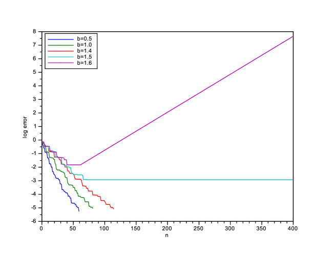
Figure 2: Evolution of $\log_{10}\left(\|F-D_{x}U_{n}-U_{n}D_{t}-b_{x}N_{x}U_{n}-b_{t}U_{n}N_{t}-U\|_{\mathfrak{S}_{2}}\right)$ as a function of $n$ for $N=20$ and different values of $b$.

Figure 3: Evolution of $\log_{10}\left(\|F-D_{x}U_{n}-U_{n}D_{t}-b_{x}N_{x}U_{n}-b_{t}U_{n}N_{t}-U\|_{\mathfrak{S}_{2}}\right)$ as a function of $n$ for $N=50$ and different values of $b$.

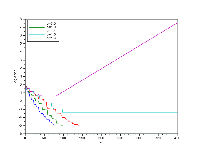
Figure 4: Evolution of $\log_{10}\left(\|F-D_{x}U_{n}-U_{n}D_{t}-b_{x}N_{x}U_{n}-b_{t}U_{n}N_{t}-U\|_{\mathfrak{S}_{2}}\right)$ as a function of $n$ for $N=100$ and different values of $b$.

We also performed another set of tests with a modified version of the Decomposition algorithm, in order to increase the threshold rate $\kappa$, in a sense which will be precised below. The modified Decomposition algorithm reads as follows for $\alpha\in[1,+\infty)$:

1. let $u_{0}=0$ and $n=1$;

2. find $(r_{n},s_{n})\in V_{x}\times V_{t}$ such that

   $$(r_{n},s_{n})\in\mathop{\mbox{\rm argmin}}_{(r,s)\in V_{x}\times V_{t}}\frac{\alpha}{2}b_{s}(r\otimes s,r\otimes s)-l(r\otimes s)-a(u_{n-1},r\otimes s);$$ (50)

3. set $u_{n}=u_{n-1}+r_{n}\otimes s_{n}$ and set $n=n+1$.

Let us point out that this algorithms is equivalent to the standard Decomposition algorithm presented in Section 5 in the case when $\alpha=1$.

Equivalently, for each $n\in{\mathbb{N}}^{*}$, $r_{n}\otimes s_{n}$ is a tensor product solution to the first iteration of the greedy algorithm applied to the symmetric coercive problem

$$\left\{\begin{array}[]{l}\mbox{find }u\in V\mbox{ such that}\\ \forall v\in V,\;\alpha b_{s}(u,v)=l(v)-a(u_{n-1},v).\\ \end{array}\right.$$

We observe that this algorithm has the same convergence properties as the standard Decomposition algorithm, i.e. there exists a threshold rate $\kappa_{\alpha}=\|\mathcal{B}_{s}^{-1}\mathcal{B}\|_{{\cal L}(V)}$ such that

• if $\|\mathcal{B}_{s}^{-1}\mathcal{B}\|_{\mathfrak{L}(V,V)}<\kappa_{\alpha}$, the algorithm converges;

• if $\|\mathcal{B}_{s}^{-1}\mathcal{B}\|_{\mathfrak{L}(V,V)}=\kappa_{\alpha}$, the algorithm does not converge, but the norm of the residual remains bounded;

• if $\|\mathcal{B}_{s}^{-1}\mathcal{B}\|_{\mathfrak{L}(V,V)}>\kappa_{\alpha}$, the algorithm does not converge, and the norm of the residual blows up.

The rate $\kappa_{\alpha}$ also seems not to depend on the dimension of the Hilbert space. Besides, $\alpha\in[1,+\infty)\mapsto\kappa_{\alpha}$ seems to be an increasing function. Thus, choosing a larger value of $\alpha$ seems to lead to an algorithm which is convergent for larger values of $b$. However, the larger $\alpha$, the smaller the rate of convergence of the algorithm for a given value of $N$ and $b$.

The figure below presents the evolution of the logarithm of the norm of the residual $\|F-D_{x}U_{n}-U_{n}D_{t}-b_{x}N_{x}U_{n}-b_{t}U_{n}N_{t}-U\|_{\mathfrak{S}_{2}}$ for the second problem for $\alpha=2$, $N=50$ and different values of $b$. The threshold value of $b$ seems to be in this case $b=2.6$.

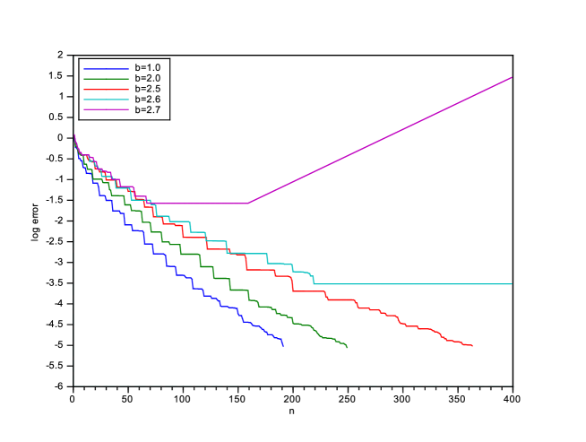
Figure 5: Evolution of $\log_{10}\left(\|F-D_{x}U_{n}-U_{n}D_{t}-b_{x}N_{x}U_{n}-b_{t}U_{n}N_{t}-U\|_{\mathfrak{S}_{2}}\right)$ as a function of $n$ for the modified Decomposition algorithm with $\alpha=2$, $N=50$ and different values of $b$.

6.3 Comparison of Galerkin, Minimax, Dual Greedy and Decomposition algorithms

In this section, we present various numerical tests performed to compare the performances of the Galerkin, Minimax, Dual Greedy and Decomposition algorithms.

6.3.1 Fixed point procedures

Before presenting the simulations done to compare the performance of the four algorithms, we will detail more precisely the fixed-point procedures used for the Galerkin, Dual and MiniMax algorithms.

Let us first present the fixed-point procedure used in the Galerkin algorithm. For all $n\in{\mathbb{N}}^{*}$, the method used to compute a pair $(r_{n},s_{n})\in V_{x}\times V_{t}$ solution to (19) is the following:

• choose $\left(r_{n}^{(0)},s_{n}^{(0)}\right)\in V_{x}\times V_{t}$ and set $m=1$;

• find $\left(r_{n}^{(m)},s_{n}^{(m)}\right)\in V_{x}\times V_{t}$ such that

  $$\left\{\begin{array}[]{l}a\left(r_{n}^{(m)}\otimes s_{n}^{(m-1)},\delta r\otimes s_{n}^{(m-1)}\right)=l\left(\delta r\otimes s_{n}^{(m-1)}\right)-a\left(u_{n-1},\delta r\otimes s_{n}^{(m-1)}\right),\;\forall\delta r\in V^{N_{x}}_{x},\\ a\left(r_{n}^{(m)}\otimes s_{n}^{(m)},r_{n}^{(m)}\otimes\delta s\right)=l\left(r_{n}^{(m)}\otimes\delta s\right)-a\left(u_{n-1},r_{n}^{(m)}\otimes\delta s\right),\;\forall\delta s\in V^{N_{t}}_{t};\\ \end{array}\right.$$

• set $m=m+1$.

All the iterations of the fixed-point procedure are well-defined. However, we have seen from Example 2.1 that there are cases where any solution $(r_{n}\otimes s_{n})\in V_{x}\times V_{t}$ of

$$\forall(\delta r,\delta s)\in V_{x}\times V_{t},\;a(r_{n}\otimes s_{n},r_{n}\otimes\delta s+\delta r\otimes s_{n})=l(r_{n}\otimes\delta s+\delta r\otimes s_{n})-a(u_{n-1},r_{n}\otimes\delta s+\delta r\otimes s_{n}),$$

satisfies $r_{n}\otimes s_{n}=0$. From Example 2.1, this is the case in particular for the first problem presented in Section 6.1 with $f\in L^{2}_{\rm per}((-1,1)^{2},{\mathbb{C}})$ being chosen such that for almost all $x,t\in(-1,1)$, $f(x,t)=\phi(x-t)$ with $\phi\in L^{2}_{\rm per}((-1,1),{\mathbb{C}})$ a real-valued odd function. The function $f=\sum_{k,l\in{\mathbb{Z}}}f_{kl}e_{k}^{x}\otimes e_{l}^{t}$ with $f_{kl}=\delta_{1,k}\delta_{-1,l}+\delta_{-1,k}\delta_{1,l}$ for all $k,l\in{\mathbb{Z}}$ is an example of such a function. On this particular example, we observe numerically that, for $n=1$, the fixed-point procedure presented above does not converge.

The practical implementation of the Galerkin algorithm requires the use of another stopping criterion as the one used in Section 6.2.1. In the numerical simulations presented in Section 6.3.2, and in the fixed-point procedures used in all the other algorithms implemented, the stopping criterion will be $m<m_{max}$ with $m_{max}=20$.

The fixed-point algorithm used for the Decomposition algorithm has been detailed in Section 6.2.1, and the one used for the MiniMax algorithm has been described in Section 4.1. The fixed-point procedure for the Dual Greedy algorithm reads as follows:

• choose $\left(\widetilde{r}_{n}^{(0)},\widetilde{s}_{n}^{(0)}\right)\in V_{x}\times V_{t}$ and set $\widetilde{m}=1$;

• while $\widetilde{m}<m_{max}$, find $\left(\widetilde{r}_{n}^{(m)},\widetilde{s}_{n}^{(m)}\right)\in V_{x}\times V_{t}$ such that for all $(\delta\widetilde{r},\delta\widetilde{s})\in V_{x}\times V_{t}$,

  $$\left\{\begin{array}[]{l}\langle\widetilde{r}_{n}^{(m)}\otimes\widetilde{s}_{n}^{(m-1)},\delta\widetilde{r}\otimes\widetilde{s}_{n}^{(m-1)}\rangle_{V}=l(\delta\widetilde{r}\otimes\widetilde{s}_{n}^{(m-1)})-a(u_{n-1},\delta\widetilde{r}\otimes\widetilde{s}_{n}^{(m-1)}),\\ \langle\widetilde{r}_{n}^{(m)}\otimes\widetilde{s}_{n}^{(m)},\widetilde{r}_{n}^{(m)}\otimes\delta\widetilde{s}\rangle_{V}=l(\widetilde{r}_{n}^{(m)}\otimes\delta\widetilde{s})-a(u_{n-1},\widetilde{r}_{n}^{(m)}\otimes\delta\widetilde{s});\\ \end{array}\right.$$

• set $\widetilde{m}=\widetilde{m}+1$;

• if $\widetilde{m}\geq m_{max}$, set $\widetilde{r}_{n}=\widetilde{r}_{n}^{(\widetilde{m})}$ and $\widetilde{s}_{n}=\widetilde{s}_{n}^{(\widetilde{m})}$;

• choose $\left(r_{n}^{(0)},s_{n}^{(0)}\right)\in V_{x}\times V_{t}$ and set $m=1$;

• while $m<m_{max}$, find $\left(r_{n}^{(m)},s_{n}^{(m)}\right)\in V_{x}\times V_{t}$ such that for all $(\delta\widetilde{r},\delta\widetilde{s})\in V_{x}\times V_{t}$,

  $$\left\{\begin{array}[]{l}a(r_{n}^{(m)}\otimes s_{n}^{(m-1)},\delta\widetilde{r}\otimes\widetilde{s}_{n})=l(\delta\widetilde{r}\otimes\widetilde{s}_{n})-a(u_{n-1},\delta\widetilde{r}\otimes\widetilde{s}_{n}),\\ a(r_{n}^{(m)}\otimes s_{n}^{(m)},\widetilde{r}_{n}\otimes\delta\widetilde{s})=l(\widetilde{r}_{n}\otimes\delta\widetilde{s})-a(u_{n-1},\widetilde{r}_{n}\otimes\delta\widetilde{s});\\ \end{array}\right.$$

• set $m=m+1$;

• if $m\geq m_{max}$, set $r_{n}=r_{n}^{(m)}$ and $s_{n}=s_{n}^{(m)}$.

6.3.2 Numerical results

We present here some numerical results obtained for the second problem introduced in Section 6.1, with $f$ chosen as in Section 6.2.2. Here $N=N_{t}=N_{x}=50$ and the different figures show the rates of convergence of the different algorithms for several values of $b=b_{x}=b_{t}$. The different values of $b$ are the following: $0.01$, $0.1$, $1$ and $2$. When $b=2$, the Decomposition algorithm does not converge.

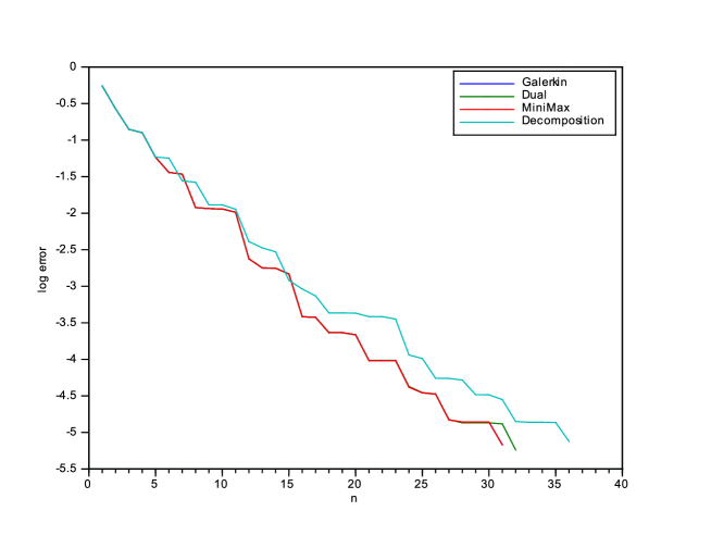
Figure 6: Evolution of $\log_{10}\left(\|F-D_{x}U_{n}-b_{x}N_{x}U_{n}-U\|_{\mathfrak{S}_{2}}\right)$ for the different algorithms as a function of $n$ with $N=50$ and $b=0.01$.

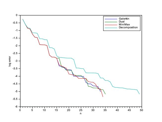
Figure 7: Evolution of $\log_{10}\left(\|F-D_{x}U_{n}-b_{x}N_{x}U_{n}-U\|_{\mathfrak{S}_{2}}\right)$ for the different algorithms as a function of $n$ with $N=50$ and $b=0.1$.

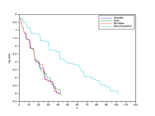
Figure 8: Evolution of $\log_{10}\left(\|F-D_{x}U_{n}-b_{x}N_{x}U_{n}-U\|_{\mathfrak{S}_{2}}\right)$ for the different algorithms as a function of $n$ with $N=50$ and $b=1$.

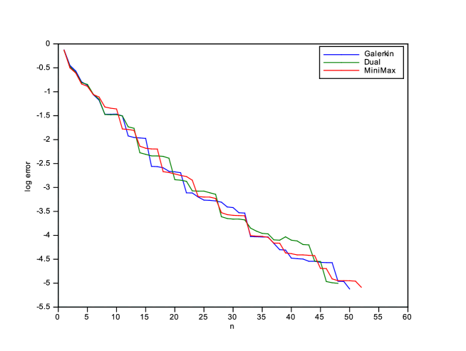
Figure 9: Evolution of $\log_{10}\left(\|F-D_{x}U_{n}-b_{x}N_{x}U_{n}-U\|_{\mathfrak{S}_{2}}\right)$ for the different algorithms as a function of $n$ with $N=50$ and $b=2$.

We observe numerically that even if the Galerkin algorithm is not well-defined through the use of the equations (19), using a fixed-point procedure as described above and stopping the procedure after a number $m_{max}$ of iterations is enough to observe good convergence properties of the algorithm. Besides, the Dual Greedy and MiniMax algorithm are almost as efficient as the Galerkin algorithm.

The Decomposition algorithm is very efficient when the antisymmetric part of the bilinear form $a(\cdot,\cdot)$ is small, but performs badly when $b$ becomes larger. Let us point out that the CPU time needed to compute one tensor product in the MiniMax or the Dual Greedy algorithms is twice the time needed in the Decomposition or the Galerkin algorithms. Thus, the Decomposition algorithm is more efficient than the Dual or the MiniMax algorithm for small antisymmetric parts of the bilinear form $a(\cdot,\cdot)$ but, when $b$ becomes too large, the algorithm behaves poorly.

7 Appendix: other algorithms

In this section, we present two other possible tracks towards the design of efficient greedy algorithms for high-dimensional non-symmetric problems, for which there is still work in progress.

7.1 An ill-defined (but converging) algorithm

In this section, we first present an algorithm whose iterations are ill-defined in general but for which we can prove the convergence in the full general case. Of course, this algorithm will not be useful in practice but we believe the proof is instructive in our context.

Let $\alpha>0$. The algorithm reads as follows:

1. set $u_{0}=0$ and $n=1$;

2. find $(r_{n},\widetilde{r}_{n},s_{n},\widetilde{s}_{n})\in V_{x}^{2}\times V_{t}^{2}$ such that

   $$\left\{\begin{array}[]{l}\displaystyle(\widetilde{r}_{n},\widetilde{s}_{n})\in\mathop{\rm argmin}_{(\widetilde{r},\widetilde{s})\in V_{x}\times V_{t}}\frac{1}{2}\|\widetilde{r}\otimes\widetilde{s}\|_{V}^{2}-l(\widetilde{r}\otimes\widetilde{s})-a(u_{n-1}+r_{n}\otimes s_{n},\widetilde{r}\otimes\widetilde{s}),\\ \displaystyle(r_{n},s_{n})\in\mathop{\rm argmin}_{(r,s)\in V_{x}\times V_{t}}\frac{\alpha}{2}\|r\otimes s\|_{V}^{2}-a(r\otimes s,\widetilde{r}_{n}\otimes\widetilde{s}_{n});\\ \end{array}\right.$$ (51)

3. set $u_{n}=u_{n-1}+r_{n}\otimes s_{n}$ and $n=n+1$.

The Euler equations associated to these coupled minimization problems read: for all $(\delta r,\delta\widetilde{r},\delta s,\delta\widetilde{s})\in V_{x}^{2}\times V_{t}^{2}$,

$$\left\{\begin{array}[]{l}\langle\widetilde{r}_{n}\otimes\widetilde{s}_{n},\widetilde{r}_{n}\otimes\delta\widetilde{s}+\delta\widetilde{r}\otimes\widetilde{s}_{n}\rangle_{V}=l(\widetilde{r}_{n}\otimes\delta\widetilde{s}+\delta\widetilde{r}\otimes\widetilde{s}_{n})-a(u_{n-1}+r_{n}\otimes s_{n},\widetilde{r}_{n}\otimes\delta\widetilde{s}+\delta\widetilde{r}\otimes\widetilde{s}_{n}),\\ \alpha\langle r_{n}\otimes s_{n},r_{n}\otimes\delta s+\delta r\otimes s_{n}\rangle_{V}=a(r_{n}\otimes\delta s+\delta r\otimes s_{n},\widetilde{r}_{n}\otimes\widetilde{s}_{n}).\\ \end{array}\right.$$ (52)

Using Lemma 1.1 and (11), these definitions imply that for all $n\in{\mathbb{N}}^{*}$,

$$\|\widetilde{r}_{n}\otimes\widetilde{s}_{n}\|_{V}=\mathop{\sup}_{(\widetilde{r},\widetilde{s})\in V_{x}\times V_{t}}\frac{l(\widetilde{r}\otimes\widetilde{s})-a(u_{n-1}+r_{n}\otimes s_{n},\widetilde{r}\otimes\widetilde{s})}{\|\widetilde{r}\otimes\widetilde{s}\|_{V}}$$ (53)

and

$$\alpha\|r_{n}\otimes s_{n}\|_{V}=\mathop{\sup}_{(r,s)\in V_{x}\times V_{t}}\frac{a(r\otimes s,\widetilde{r}_{n}\otimes\widetilde{s}_{n})}{\|r\otimes s\|_{V}}.$$ (54)

Indeed, for the first equality, one has to consider the symmetric coercive continuous bilinear form $a^{1}(\cdot,\cdot)=\langle\cdot,\cdot\rangle_{V}$ and the continuous linear form $l^{1}(\cdot)=l(\cdot)-a(u_{n-1}+r_{n}\otimes s_{n},\cdot)$. For the second equality, the symmetric coercive continuous bilinear form to consider is $a^{2}(\cdot,\cdot)=\alpha\langle\cdot,\cdot\rangle_{V}$ and the continuous linear form is $l^{2}(\cdot)=a(\cdot,\widetilde{r}_{n}\otimes\widetilde{s}_{n})$.

The following result holds:

Proposition 7.1.

Let us assume that the iterations of algorithm (51) are well-defined for all $n\in{\mathbb{N}}^{*}$. Then, $(u_{n})_{n\in{\mathbb{N}}^{*}}$ converges to $u$ in the sense of the injective norm:

$$\|u-u_{n}\|_{i\mathcal{A}}=\mathop{\sup}_{(\widetilde{r},\widetilde{s})\in V_{x}\times V_{t}}\frac{a(u-u_{n},\widetilde{r}\otimes\widetilde{s})}{\|\widetilde{r}\otimes\widetilde{s}\|_{V}}\mathop{\longrightarrow}_{n\to\infty}0.$$

Proof.

Let us first remark that, using (53),

$$\|u-u_{n}\|_{i\mathcal{A}}=\mathop{\sup}_{(\widetilde{r},\widetilde{s})\in V_{x}\times V_{t}}\frac{a(u-u_{n},\widetilde{r}\otimes\widetilde{s})}{\|\widetilde{r}\otimes\widetilde{s}\|_{V}}=\|\widetilde{r}_{n}\otimes\widetilde{s}_{n}\|_{V}.$$

Thus, it is sufficient to prove that the sequence $(\|\widetilde{r}_{n}\otimes\widetilde{s}_{n}\|_{V})_{n\in{\mathbb{N}}^{*}}$ converges to $0$ as $n$ goes to infinity. Let us first prove that this sequence is non-increasing. Let $n\geq 2$. From the Euler equation (52) associated to the minimization problem defining $(\widetilde{r}_{n},\widetilde{s}_{n})$, it holds that

$$\|\widetilde{r}_{n}\otimes\widetilde{s}_{n}\|_{V}^{2}=l(\widetilde{r}_{n}\otimes\widetilde{s}_{n})-a(u_{n-1}+r_{n}\otimes s_{n},\widetilde{r}_{n}\otimes\widetilde{s}_{n}).$$ (55)

Besides, using (53) at iteration $n-1$, we obtain

$$\|\widetilde{r}_{n-1}\otimes\widetilde{s}_{n-1}\|_{V} = \mathop{\sup}_{(\widetilde{r},\widetilde{s})\in V_{x}\times V_{t},\;\widetilde{r}\otimes\widetilde{s}\neq 0}\frac{l(\widetilde{r}\otimes\widetilde{s})-a(u_{n-1},\widetilde{r}\otimes\widetilde{s})}{\|\widetilde{r}\otimes\widetilde{s}\|_{V}}$$

$$\geq \frac{l(\widetilde{r}_{n}\otimes\widetilde{s}_{n})-a(u_{n-1},\widetilde{r}_{n}\otimes\widetilde{s}_{n})}{\|\widetilde{r}_{n}\otimes\widetilde{s}_{n}\|_{V}},$$

which, using (55), leads to

$$\|\widetilde{r}_{n}\otimes\widetilde{s}_{n}\|_{V}^{2}\leq\|\widetilde{r}_{n-1}\otimes\widetilde{s}_{n-1}\|_{V}\|\widetilde{r}_{n}\otimes\widetilde{s}_{n}\|_{V}-a(r_{n}\otimes s_{n},\widetilde{r}_{n}\otimes\widetilde{s}_{n}).$$

Using the second Euler equation (52) defining $(r_{n},s_{n})$, we have that $\alpha\|r_{n}\otimes s_{n}\|_{V}^{2}=a(r_{n}\otimes s_{n},\widetilde{r}_{n}\otimes\widetilde{s}_{n})$. Finally, it holds that

$$\|\widetilde{r}_{n}\otimes\widetilde{s}_{n}\|_{V}^{2}\leq\|\widetilde{r}_{n}\otimes\widetilde{s}_{n}\|_{V}\|\widetilde{r}_{n-1}\otimes\widetilde{s}_{n-1}\|_{V}-\alpha\|r_{n}\otimes s_{n}\|_{V}^{2}.$$ (56)

This implies that the sequence $(\|\widetilde{r}_{n}\otimes\widetilde{s}_{n}\|_{V})_{n\in{\mathbb{N}}^{*}}$ is non-increasing and thus converges towards a limit $z\geq 0$. Let us argue by contradiction and assume that $z>0$. Dividing by $\|\widetilde{r}_{n}\otimes\widetilde{s}_{n}\|_{V}$ equation (56), we obtain

$$\alpha\frac{\|r_{n}\otimes s_{n}\|_{V}^{2}}{\|\widetilde{r}_{n}\otimes\widetilde{s}_{n}\|_{V}}\leq\|\widetilde{r}_{n-1}\otimes\widetilde{s}_{n-1}\|_{V}-\|\widetilde{r}_{n}\otimes\widetilde{s}_{n}\|_{V}.$$

Since we have assumed that $\|\widetilde{r}_{n}\otimes\widetilde{s}_{n}\|_{V}\geq z>0$ for all $n\in{\mathbb{N}}^{*}$, the series of general term $(\|r_{n}\otimes s_{n}\|_{V}^{2})_{n\in{\mathbb{N}}^{*}}$ converges and $\displaystyle\|r_{n}\otimes s_{n}\|_{V}\mathop{\longrightarrow}_{n\to\infty}0$. Using (54), this implies that for all $(r,s)\in V_{x}\times V_{t}$,

$$a(r\otimes s,\widetilde{r}_{n}\otimes\widetilde{s}_{n})\mathop{\longrightarrow}_{n\to\infty}0.$$

Using assumption (A1) and the fact that $(\|\widetilde{r}_{n}\otimes\widetilde{s}_{n}\|_{V})_{n\in{\mathbb{N}}^{*}}$ is bounded, we have

$$\forall w\in V,\;a(w,\widetilde{r}_{n}\otimes\widetilde{s}_{n})\mathop{\longrightarrow}_{n\to\infty}0.$$

Since we have assumed that the operator $\mathcal{A}$ is bijective, it is surjective on $V$, and the sequence $(\widetilde{r}_{n}\otimes\widetilde{s}_{n})_{n\in{\mathbb{N}}^{*}}$ weakly converges to $0$ in $V$.

Using (53), it holds that for all $n\in{\mathbb{N}}^{*}$,

$$\|\widetilde{r}_{n}\otimes\widetilde{s}_{n}\|_{V}^{2}=l(\widetilde{r}_{n}\otimes\widetilde{s}_{n})-a(u_{n},\widetilde{r}_{n}\otimes\widetilde{s}_{n})=l(\widetilde{r}_{n}\otimes\widetilde{s}_{n})-a\left(\sum_{k=1}^{n}r_{k}\otimes s_{k},\widetilde{r}_{n}\otimes\widetilde{s}_{n}\right).$$

Since $(\widetilde{r}_{n}\otimes\widetilde{s}_{n})_{n\in{\mathbb{N}}^{*}}$ weakly converges to $0$ in $V$, necessarily $\displaystyle l(\widetilde{r}_{n}\otimes\widetilde{s}_{n})\mathop{\longrightarrow}_{n\to\infty}0$. Besides, using (54), we have

$$\left|a\left(\sum_{k=1}^{n}r_{k}\otimes s_{k},\widetilde{r}_{n}\otimes\widetilde{s}_{n}\right)\right| \leq \sum_{k=1}^{n}\left|a\left(r_{k}\otimes s_{k},\widetilde{r}_{n}\otimes\widetilde{s}_{n}\right)\right|$$

$$\leq \alpha\sum_{k=1}^{n}\|r_{k}\otimes s_{k}\|_{V}\|r_{n}\otimes s_{n}\|_{V}$$

$$\leq \alpha\left(\sum_{k=1}^{n}\|r_{k}\otimes s_{k}\|_{V}^{2}\right)^{1/2}(n\|r_{n}\otimes s_{n}\|_{V}^{2})^{1/2}.$$

Since the series of general term $(\|r_{n}\otimes s_{n}\|_{V}^{2})_{n\in{\mathbb{N}}^{*}}$ is convergent, the sequence $\left(\sum_{k=1}^{n}\|r_{k}\otimes s_{k}\|_{V}^{2}\right)_{n\in{\mathbb{N}}^{*}}$ is bounded and there exists a subsequence of $(n\|r_{n}\otimes s_{n}\|_{V}^{2})_{n\in{\mathbb{N}}^{*}}$ which converges to $0$. Thus, there exists a subsequence of $(\|\widetilde{r}_{n}\otimes\widetilde{s}_{n}\|_{V})_{n\in{\mathbb{N}}^{*}}$ converging to $0$ and since the whole sequence converges to $z$, we have $z=0$ by uniqueness of the limit. We obtain a contradiction. ∎

Remark 7.1.

Unfortunately, as announced in the beginning of this section, in general, the iterations of algorithm (51) are not well-defined in the sense that there may not exist a solution $(r_{n},\widetilde{r}_{n},s_{n},\widetilde{s}_{n})\in V_{x}^{2}\times V_{t}^{2}$ of the coupled minimization problems. Numerically, we can observe that if we use a coupled fixed-point algorithm similar to the one presented for the Minimax algorithm, the procedure does not converge in general. Finding a suitable way to adapt these ideas in an implementable well-defined algorithm is work in progress.

Remark 7.2.

When the bilinear form $a(\cdot,\cdot)$ is symmetric and coercive, all the iterations of algorithm (51) are well-defined. If $\langle\cdot,\cdot\rangle_{V}$ is chosen to be equal to $a(\cdot,\cdot)$, the second equation of (52) implies that $r_{n}\otimes s_{n}=\frac{1}{\alpha}\widetilde{r}_{n}\otimes\widetilde{s}_{n}$ and the first equation of (52) can be rewritten as: for all $(\delta\widetilde{r},\delta\widetilde{s})\in V_{x}\times V_{t}$,

$$\left(1+\frac{1}{\alpha}\right)\langle\widetilde{r}_{n}\otimes\widetilde{s}_{n},\widetilde{r}_{n}\otimes\delta\widetilde{s}+\delta\widetilde{r}\otimes\widetilde{s}_{n}\rangle_{V}=l(\widetilde{r}_{n}\otimes\delta\widetilde{s}+\delta\widetilde{r}\otimes\widetilde{s}_{n})-\langle u_{n-1},\widetilde{r}_{n}\otimes\delta\widetilde{s}+\delta\widetilde{r}\otimes\widetilde{s}_{n}\rangle_{V}.$$

This Euler equation is similar to the Euler equation of the first iteration of the standard greedy algorithm applied to the symmetric coercive problem:

$$\left\{\begin{array}[]{l}\mbox{find }\widetilde{u}\in V\mbox{ such that}\\ \forall v\in V,\left(1+\;\frac{1}{\alpha}\right)\langle\widetilde{u},v\rangle_{V}=l(v)-\langle u_{n-1},v\rangle_{V}.\\ \end{array}\right.$$

Thus, if we consider now the following (well-defined) algorithm

1. set $u_{0}=0$ and $n=1$;

2. find $(r_{n},s_{n})\in V_{x}\times V_{t}$ such that

   $$(r_{n},s_{n})\in\mathop{\mbox{argmin}}_{(r,s)\in V_{x}\times V_{t}}\frac{\lambda}{2}\|r\otimes s\|_{V}^{2}-l(r\otimes s)-\langle u_{n-1},v\rangle_{V};$$

3. set $u_{n}=u_{n-1}+r_{n}\otimes s_{n}$ and $n=n+1$,

following the proof of Proposition 7.1, we can prove that the sequence $(u_{n})_{n\in{\mathbb{N}}^{*}}$ converges to ${\cal L}$ in the sense of the injective norm as soon as $\lambda>1$. Let us point out that when $\lambda=1$, this algorithm is identical to the standard greedy algorithm applied to the symmetric coercive problem

$$\left\{\begin{array}[]{l}\mbox{find }\widetilde{u}\in V\mbox{ such that}\\ \forall v\in V,\langle\widetilde{u},v\rangle_{V}=l(v).\\ \end{array}\right.$$

7.2 Link with a symmetric formulation

Let us now present another approach, for which no convergence result have been proved so far. The idea is based on the article [7] by Cohen, Dahmen and Welper, where the objective was to develop stable formulations of multiscale convection-diffusion equations.

The principle of the method is to reformulate the antisymmetric problem (16) defined on the Hilbert space $V$, as a symmetric problem defined on the Hilbert space $V\times V$. Indeed, it is proved in [7] that the unique solution of the problem

$$\left\{\begin{array}[]{l}\mbox{find }(v,\widetilde{v})\in V\times V\mbox{ such that}\\ a(w,\widetilde{v})=0,\quad\forall w\in V,\\ a(v,\widetilde{w})-\langle R_{V}\widetilde{v},\widetilde{w}\rangle=l(\widetilde{w}),\quad\forall\widetilde{w}\in V,\\ \end{array}\right.$$ (57)

is $(v,\widetilde{v})=(u,0)$ where $u$ is the unique solution of (16).

This new problem is now symmetric. It is equivalent to the following problem

$$\left\{\begin{array}[]{l}\mbox{find }(v,\widetilde{v})\in V\times V\mbox{ such that}\\ \left(\begin{array}[]{cc}0&A^{*}\\ A&-R_{V}\\ \end{array}\right)\left(\begin{array}[]{c}v\\ \widetilde{v}\\ \end{array}\right)=\left(\begin{array}[]{c}0\\ L\\ \end{array}\right)\mbox{ in }V^{\prime}\times V^{\prime}.\\ \end{array}\right.$$

This new formulation of the problem is symmetric, but not coercive. No convergence results exist for greedy methods in this framework. However, the situation seems more encouraging than in the original non-symmetric case. It is to be noted though that the use of a simple Galerkin algorithm, similar to the one introduced in Section 2.3, does not work in this case either. More subtle algorithms need to be designed in this case as well, and this is currently work in progress.

References

- [1] A. Ammar, B. Mokdad, F. Chinesta, and R. Keunings. A new family of solvers for some classes of multidimensional partial differential equations encountered in kinetic theory modeling of complex fluids. Journal of Non-Newtonian Fluid Mechanics, 139:153–176, 2006.
- [2] R.E. Bellman. Dynamic Programming. Princeton University Press, 1957.
- [3] G. Bonithon and A. Nouy. Tensor-based methods and proper generalized decompositions for the numerical solution of high-dimensional problems: alternative definitions. preprint, hal.archives-ouvertes.fr/hal-00664061, 2012.
- [4] A. Buffa, Y. Maday, A.T. Patera, C. Prud’homme, and G. Turinici. A priori convergence of the greedy algorithm for the parametrized reduced basis. ESAIM: Mathematical Modelling and Numerical Analysis, 46:595–603, 2012.
- [5] E Cancès, V. Ehrlacher, and T. Lelièvre. Convergence of a greedy algorithm for high-dimensional convex problems. Mathematical Models and Methods in Applied Sciences, 21:2433–2467, 2011.
- [6] A. Chkifa, A. Cohen, R. DeVore, and C. Schwab. Sparse Adaptive Taylor Approximation Algorithms for Parametric and Stochastic Elliptic PDEs. Submitted, 2011.
- [7] A. Cohen, W. Dahmen, and G. Welper. Adaptivity and variational stabilization for convection-diffusion equations. ESAIM: Mathematical Modelling and Numerical Analysis, 46:1247–1273, 2012.
- [8] J. Diestel and J. Fourie, J.H. ans Swart. The Metric Theory of Tensor Products. American Mathematical Society, 2008.
- [9] A. Falco, L. Hilario, N. Montès, and M.C. Mora. Numerical strategies for the Galerkin-Proper Generalized Decomposition Method. Mathematical and Computer Modelling (in press), 2012.
- [10] L. Figueroa and E. Suli. Greedy Approximation of High-Dimensional Ornstein-Uhlenbeck Operators. Foundations of Computational Mathematics, 12:573–623, 2012.
- [11] W. Hackbusch. Tensor Spaces and Numerical Tensor Calculus. Springer, 2012.
- [12] P. Ladevèze. Nonlinear computational structural mechanics: new approaches and non-incremental methods of calculation. Springer, Berlin, 1999.
- [13] C. Le Bris, T. Lelièvre, and Y. Maday. Results and Questions on a Nonlinear Approximation Approach for Solving High-dimensional Partial Differential Equations. Constructive Approximation, 30:621–651, 2009.
- [14] A. Lozinski. Interplay between PGD and greedy approximation algorithms for high-dimensional PDEs: symmetric and not symmetric cases. http://website.ec-nantes.fr/reduc/, 2010.
- [15] A. Nouy. Recent developments in spectral stochastic methods for the numerical solution of stochastic partial differential equations. Archives of Computational Methods in Engineering, 16:251–285, 2009.
- [16] A. Nouy. A priori model reduction through Proper Generalized Decomposition for solving time-dependent partial differential equations. Computer Methods in Applied Mechanics and Engineering, 199:1603–1626, 2010.
- [17] A. Nouy. A priori model reduction through Proper Generalized Decomposition for solving time-dependent partial differential equations. Computer Methods in Applied Mechanics and Engineering, 199:1603–1626, 2010.
- [18] A. Nouy and A. Falco. Proper Generalized Decomposition for Nonlinear Convex Problems in Tensor Banach Spaces. Numerische Mathematik, 121:503–530, 2012.
- [19] L. Skrzypek. Uniqueness of Minimal Projections in Smooth Matrix Spaces. Journal of Approximation Theory, 107:315–336, 2000.
- [20] V.N. Temlyakov. Greedy Approximation. Acta Numerica, 17:235–409, 2008.
- [21] T. von Petersdorff and C. Schwab. Numerical solution of parabolic equations in high dimensions. M2AN Mathematical Modelling and Numerical Analysis, 38:93–127, 2004.