Variance bounding and geometric ergodicity of Markov chain Monte Carlo kernels for approximate Bayesian computation

Abstract

Approximate Bayesian computation has emerged as a standard computational tool when dealing with the increasingly common scenario of completely intractable likelihood functions in Bayesian inference. We show that many common Markov chain Monte Carlo kernels used to facilitate inference in this setting can fail to be variance bounding, and hence geometrically ergodic, which can have consequences for the reliability of estimates in practice. This phenomenon is typically independent of the choice of tolerance in the approximation. We then prove that a recently introduced Markov kernel in this setting can inherit variance bounding and geometric ergodicity from its intractable Metropolis–Hastings counterpart, under reasonably weak and manageable conditions. We show that the computational cost of this alternative kernel is bounded whenever the prior is proper, and present indicative results on an example where spectral gaps and asymptotic variances can be computed, as well as an example involving inference for a partially and discretely observed, time-homogeneous, pure jump Markov process. We also supply two general theorems, one of which provides a simple sufficient condition for lack of variance bounding for reversible kernels and the other provides a positive result concerning inheritance of variance bounding and geometric ergodicity for mixtures of reversible kernels.

1 Introduction

Approximate Bayesian computation refers to branch of Monte Carlo methodology that uses the ability to simulate data according to a parametrized likelihood function in lieu of computation of that likelihood to perform approximate, parametric Bayesian inference. These methods have been used in an increasingly diverse range of applications since their inception in the context of population genetics (Tavaré et al., 1997; Pritchard et al., 1999), particularly in cases where the likelihood function is either impossible or computationally prohibitive to evaluate.

We are in a standard Bayesian setting with data $y\in\mathsf{Y}$, a parameter space $\Theta$, a prior $p:\Theta\rightarrow\mathbb{R}_{+}$ and for each $\theta\in\Theta$ a likelihood $f_{\theta}:\mathsf{Y}\rightarrow\mathbb{R}_{+}$. We assume $\mathsf{Y}$ is a metric space and consider the artificial likelihood

$$f_{\theta}^{\epsilon}(y)=V(\epsilon)^{-1}\int_{\mathsf{Y}}I\left(y\in B_{\epsilon,x}\right)f_{\theta}(x)\mathrm{d}x=V(\epsilon)^{-1}f_{\theta}\left(B_{\epsilon,y}\right),$$ (1)

which is commonly employed in approximate Bayesian computation. The value of $\epsilon$ can be interpreted as the tolerance of the approximation. Here, $B_{r,z}$ denotes a metric ball of radius $r$ around $z$, $V(r)=\int_{\mathsf{Y}}I\left(x\in B_{r,0}\right)\mathrm{d}x$ denotes the volume of a ball of radius $r$ in $\mathcal{\mathsf{Y}}$ and $I$ denotes the indicator function. We slightly abuse language by referring to densities as distributions, and where convenient, employ the measure-theoretic notation $\mu(A)=\int_{A}\mu(d\lambda)$. We consider situations in which both $\epsilon$ and $y$ are fixed, and so define functions $h:\Theta\rightarrow[0,1]$ and $w:\mathsf{Y}\rightarrow[0,1]$ by

$$h(\theta)=f_{\theta}\left(B_{\epsilon,y}\right)$$ (2)

and $w(x)=I\left(y\in B_{\epsilon,x}\right)$ to simplify the presentation. The value $h(\theta)$ can be interpreted as the probability of ‘hitting’ $B_{\epsilon,y}$ with a sample drawn from $f_{\theta}$.

While the artificial likelihood (1) is also intractable in general, the approximate posterior it induces, $\pi(\theta)=h(\theta)p(\theta)/\int_{\Theta}h(\vartheta)p(\vartheta){\rm d}\vartheta$, can be dealt with using constrained versions of standard methods when sampling from $f_{\theta}$ is possible for any $\theta\in\Theta$ (see, e.g., Marin et al., 2012). In particular, one typically uses $f_{\theta}$ as a proposal in such a way that its explicit computation is avoided. We are often interested in computing $\pi(\varphi)=\int_{\Theta}\varphi(\theta)\pi(\theta){\rm d\theta}$, the posterior expectation of some function $\varphi$, and it is this type of quantity that can be approximated using Monte Carlo methodology. We focus on one such method, Markov chain Monte Carlo, whereby a Markov chain is constructed by sampling iteratively from an irreducible Markov kernel $P$ with unique stationary distribution $\pi$. We can use such a chain directly to estimate $\pi(\varphi)$ using appropriately normalized partial sums, i.e., given the realization $\theta_{1},\theta_{2},\ldots$ of a chain started at $\theta_{0}$, where $\theta_{i}\sim P(\theta_{i-1},\cdot)$ for $i\in\mathbb{N}$ we compute the estimate

$$\frac{1}{m}\sum_{i=1}^{m}\varphi(\theta_{i}),$$ (3)

for some $m$. Alternatively, the Markov kernels can be used within other methods such as sequential Monte Carlo (Del Moral et al., 2006). In the former case, it is desirable that a central limit theorem holds for (3) and that the asymptotic variance ${\rm var}(P,\varphi)$ of (3) be reasonably small, while in the latter it is desirable that the kernel be geometrically ergodic, i.e., $P^{m}(\theta_{0},\cdot)$ converges at a geometric rate in $m$ to $\pi$ in total variation where $P^{m}$ is the $m$-fold iterate of $P$ (see, e.g., Roberts & Rosenthal, 2004; Meyn & Tweedie, 2009), at least because this property is often assumed in analyses (see, e.g., Jasra & Doucet, 2008; Whiteley, 2012). In addition, consistent estimation of ${\rm var}(P,\varphi)$ is well established (Hobert et al., 2002; Jones et al., 2006; Bednorz & Łatuszyński, 2007; Flegal & Jones, 2010) for geometrically ergodic chains.

Motivated by these considerations, we study both the variance bounding (Roberts & Rosenthal, 2008) and geometric ergodicity properties of a number of reversible kernels used for approximate Bayesian computation. For reversible $P$, a central limit theorem holds for all $\varphi\in L^{2}(\pi)$ if and only if $P$ is variance bounding (Roberts & Rosenthal, 2008, Theorem 7), where $L^{2}(\pi)$ is the space of square-integrable functions with respect to $\pi$. Of course, reversible kernels that are not variance bounding can still produce Markov chains where (3) satisfies a central limit theorem for some, but not all, functions in $L^{2}(\pi)$.

Much of the literature seeks to control the trade-off associated with the quality of approximation (1), controlled by $\epsilon$ and manipulation of $y$, and counteracting computational difficulties (see, e.g., Fearnhead & Prangle, 2012). We address here a separate issue, namely that many Markov kernels used in this context are neither variance bounding nor geometrically ergodic, for any finite $\epsilon$ in rather general situations when using ‘local’ proposal distributions.

As a partial remedy to the problems identified by this negative result, we also show that under reasonably mild conditions, a kernel proposed in Lee et al. (2012) can inherit variance bounding and geometric ergodicity from its intractable Metropolis–Hastings (Metropolis et al., 1953; Hastings, 1970) counterpart. This allows for the specification of a broad class of models for which we can be assured this particular kernel will be geometrically ergodic. In addition, conditions ensuring inheritance of either property can be met without knowledge of $f_{\theta}$, e.g. by using a symmetric proposal and a prior that is continuous, everywhere positive and has exponential or heavier tails.

To assist in the interpretation of results and the quantitative example in the discussion, we provide some background on the spectral properties of variance bounding and geometrically ergodic Markov kernels. Both variance bounding and geometric ergodicity of a reversible Markov kernel $P$ are related to $\sigma_{0}(P)$, the spectrum of $P$ considered as an operator on $L_{0}^{2}(\pi)$, the restriction of $L^{2}(\pi)$ to zero-mean functions (see, e.g., Geyer & Mira, 2000; Mira, 2001). Variance bounding is equivalent to $\sup\sigma_{0}(P)<1$ (Roberts & Rosenthal, 2008, Theorem 14) and geometric ergodicity is equivalent to $\sup|\sigma_{0}(P)|<1$ (Kontoyiannis & Meyn, 2012; Roberts & Rosenthal, 1997, Theorem 2.1). The spectral gap ${\rm Gap}(P)=1-\sup|\sigma_{0}(P)|$ of a geometrically ergodic kernel is closely related to its aforementioned geometric rate of convergence to $\pi$, with faster rates associated with larger spectral gaps. In particular, its convergence in total variation satisfies for some $1>\rho\geq\sup|\sigma_{0}(P)|$ and some function $C_{\rho}:\Theta\rightarrow\mathbb{R}_{+}$ (c.f. Baxendale, 2005, Section 6)

$$\|\pi(\cdot)-P^{m}(\theta_{0},\cdot)\|_{{\rm TV}}\leq C_{\rho}(\theta_{0})\rho^{m}.$$ (4)

2 The Markov kernels

In this section we describe the algorithmic specification of the $\pi$-invariant Markov kernels under study. The algorithms specify how to sample from each kernel; in each, a candidate $\vartheta$ is proposed according to a common proposal $q(\theta,\cdot)$ and accepted or rejected, possibly along with other auxiliary variables, using simulations from the likelihoods $f_{\vartheta}$ and $f_{\theta}$. We assume that for all $\theta\in\Theta$, $q(\theta,\cdot)$ and $p$ are densities with respect to a common dominating measure, e.g. the Lebesgue or counting measures.

The first and simplest Markov kernel in this setting was proposed in Marjoram et al. (2003), and is a special case of a ‘pseudo-marginal’ kernel (Beaumont, 2003; Andrieu & Roberts, 2009). Such kernels have been used in the context of approximate Bayesian computation for the estimation of parameters in speciation models (Becquet & Przeworski, 2007; Chen et al., 2009; Li et al., 2010; Kim et al., 2011), and as a methodological component within an SMC sampler (Del Moral et al., 2012; Drovandi & Pettitt, 2011). They evolve on $\Theta\times\mathsf{Y}^{N}$ and involve sampling auxiliary variables $z_{1:N}\sim f_{\vartheta}^{\otimes N}$ for a fixed $N\in\mathbb{N}$. We denote kernels of this type for any $N$ by $P_{\ref{alg:pm_kernel_1},N}$, and describe their simulation in Algorithm 1. It is readily verified (Beaumont, 2003; Andrieu & Roberts, 2009) that $P_{\ref{alg:pm_kernel_1},N}$ is reversible with respect to

$$\bar{\pi}(\theta,x_{1:N})\propto p(\theta)\prod_{j=1}^{N}f_{\theta}(x_{j})\frac{1}{N}\sum_{j=1}^{N}w(x_{j}),$$

and we have $\bar{\pi}(\theta)=\int\bar{\pi}(\theta,x_{1:N}){\rm d}x_{1:N}=\pi(\theta)$, i.e., the $\theta$-marginal of $\bar{\pi}$ is $\pi(\theta).$

Algorithm 1 To sample from $P_{\ref{alg:pm_kernel_1},N}(\theta,x_{1:N};\cdot)$

1. Sample $\vartheta\sim q(\theta,\cdot)$ and $z_{1:N}\sim f_{\vartheta}^{\otimes N}$.

2. With probability

   $$1\wedge\frac{p(\vartheta)q(\vartheta,\theta)\sum_{j=1}^{N}w(z_{j})}{p(\theta)q(\theta,\vartheta)\sum_{j=1}^{N}w(x_{j})},$$

   output $(\vartheta,z_{1:N})$. Otherwise, output $(\theta,x_{1:N})$.

In Lee et al. (2012), two alternative kernels were proposed in this context, both of which evolve on $\Theta$. One, denoted $P_{\ref{alg:pm_kernel_2},N}$ and described in Algorithm 2, is an alternative pseudo-marginal kernel that in addition to sampling $z_{1:N}\sim f_{\vartheta}^{\otimes N}$, also samples auxiliary variables $x_{1:N-1}\sim f_{\theta}^{\otimes N-1}$. Detailed balance can be verified directly upon interpreting $\sum_{j=1}^{N}w(z_{j})$ and $\sum_{j=1}^{N-1}w(x_{j})$ as Binomial$\left\{N,h(\vartheta)\right\}$ and Binomial$\left\{N-1,h(\theta)\right\}$ random variables respectively. The other kernel, denoted $P_{\ref{alg:1_hit_kernel}}$ and described in Algorithm 3, also involves sampling according to $f_{\theta}$ and $f_{\vartheta}$ but does not sample a fixed number of auxiliary variables. This kernel also satisfies detailed balance (Lee, 2012, Proposition 1).

Algorithm 2 To sample from $P_{\ref{alg:pm_kernel_2},N}(\theta,\cdot)$

1. Sample $\vartheta\sim q(\theta,\cdot)$, $x_{1:N-1}\sim f_{\theta}^{\otimes N-1}$ and $z_{1:N}\sim f_{\vartheta}^{\otimes N}$.

2. With probability

   $$1\wedge\frac{p(\vartheta)q(\vartheta,\theta)\sum_{j=1}^{N}w(z_{j})}{p(\theta)q(\theta,\vartheta)\left\{1+\sum_{j=1}^{N-1}w(x_{j})\right\}},$$

   output $\vartheta$. Otherwise, output $\theta$.

Algorithm 3 To sample from $P_{\ref{alg:1_hit_kernel}}(\theta,\cdot)$

1. Sample $\vartheta\sim q(\theta,\cdot)$.

2. With probability

   $$1-\left\{1\wedge\frac{p(\vartheta)q(\vartheta,\theta)}{p(\theta)q(\theta,\vartheta)}\right\},$$

   stop and output $\theta$.

3. For $i=1,2,\ldots$ until $\sum_{j=1}^{i}w(z_{j})+w(x_{j})\geq 1$, sample $x_{i}\sim f_{\theta}$ and $z_{i}\sim f_{\vartheta}$. Set $N\leftarrow i$.

4. If $w(z_{N})=1$, output $\vartheta$. Otherwise, output $\theta$.

Our first results in Section 3 concern $P_{\ref{alg:pm_kernel_1},N}$ and $P_{\ref{alg:pm_kernel_2},N}$. One typically expects better performance from these kernels for larger values of $N$ (see, e.g, Andrieu & Vihola, 2012), and such behaviour can often be demonstrated empirically. However, we establish that both of these kernels can nevertheless fail to be variance bounding regardless of the value of $N$ when $q$ proposes moves locally. This suggests that increasing $N$ may only bring an improvement up to a certain point. On the other hand, subsequent results for $P_{\ref{alg:1_hit_kernel}}$ show that by expending more computational effort in particular places one can successfully inherit variance bounding and/or geometric ergodicity from $P_{{\rm MH}}$, the Metropolis–Hastings kernel with proposal $q$.

Because many of our positive results for $P_{\ref{alg:1_hit_kernel}}$ are in relation to $P_{{\rm MH}}$, we provide the algorithmic specification for sampling from $P_{{\rm MH}}$ in Algorithm 4. In the approximate Bayesian computation setting, use of $P_{{\rm MH}}$ is ruled out by assumption since $h$ cannot be computed. However, the preceding kernels are all, in some sense, exact approximations of $P_{{\rm MH}}$.

Algorithm 4 To sample from $P_{{\rm MH}}(\theta,\cdot)$

1. Sample $\vartheta\sim q(\theta,\cdot)$.

2. With probability

   $$1\wedge\frac{p(\vartheta)h(\vartheta)q(\vartheta,\theta)}{p(\theta)h(\theta)q(\theta,\vartheta)},$$

   output $\vartheta$. Otherwise, output $\theta$.

The kernels share a similar structure, and $P_{\ref{alg:pm_kernel_2},N}$, $P_{\ref{alg:1_hit_kernel}}$ and $P_{{\rm MH}}$ can each be written as

$$P(\theta,{\rm d}\vartheta)=q(\theta,{\rm d\vartheta)}\alpha(\theta,\vartheta)+\left\{1-\int_{\Theta}q(\theta,{\rm d}\theta^{\prime})\alpha(\theta,\theta^{\prime})\right\}\delta_{\theta}({\rm d}\vartheta),$$ (5)

where only the acceptance probability $\alpha(\theta,\vartheta)$ differs. $P_{\ref{alg:pm_kernel_1},N}$ can be represented similarly, with modifications to account for its evolution on the extended space $\Theta\times\mathsf{Y}^{N}$. The representation (5) is used extensively in our analysis, and we have for $P_{\ref{alg:pm_kernel_2},N}$, $P_{\ref{alg:1_hit_kernel}}$ and $P_{{\rm MH}}$, respectively

$$\alpha_{\ref{alg:pm_kernel_2},N}(\theta,\vartheta) =\int_{\mathsf{Y}^{N}}\int_{\mathsf{Y}^{N-1}}\left[1\wedge\frac{c(\vartheta,\theta)\sum_{j=1}^{N}w(z_{j})}{c(\theta,\vartheta)\left\{1+\sum_{j=1}^{N-1}w(x_{j})\right\}}\right]f_{\theta}^{\otimes N-1}({\rm d}x_{1:N-1})f_{\vartheta}^{\otimes N}({\rm d}z_{1:N}),$$ (6)

$$\alpha_{\ref{alg:1_hit_kernel}}(\theta,\vartheta) =\left\{1\wedge\frac{c(\vartheta,\theta)}{c(\theta,\vartheta)}\right\}\frac{h(\vartheta)}{h(\theta)+h(\vartheta)-h(\theta)h(\vartheta)},$$ (7)

$$\alpha_{{\rm MH}}(\theta,\vartheta) =1\wedge\frac{c(\vartheta,\theta)h(\vartheta)}{c(\theta,\vartheta)h(\theta)},$$ (8)

where $c(\theta,\vartheta)=p(\theta)q(\theta,\vartheta)$ and (7) is obtained, e.g., in Lee (2012). Finally, we reiterate that all the kernels satisfy detailed balance and are therefore reversible.

3 Theoretical properties

We assume that $\Theta$ is a metric space, and that

$$H=\int_{\Theta}p(\theta)h(\theta)\mathrm{d}\theta$$ (9)

satisfies $H\in(0,\infty)$ so $\pi$ is well defined. We allow $p$ to be improper, i.e., for $\int_{\Theta}p(\theta){\rm d}\theta$ to be infinite but when it is proper we assume it is normalized so $\int_{\Theta}p(\theta){\rm d}\theta=1$. We define the collection of local proposals as

$$\mathcal{Q}=\left\{q\>:\>\text{for all }\delta>0,\>\text{there exists }r\in(0,\infty)\>\text{such that for all }\theta\in\Theta,\>q\left(\theta,B_{r,\theta}^{\complement}\right)<\delta\right\},$$ (10)

which encompasses a broad number of common choices in practice, e.g., $q$ being a random walk. This corresponds to the tightness of centred proposals $q$.

We denote by $\mathcal{V}$ and $\mathcal{G}$ the collections of reversible kernels that are respectively variance bounding (Roberts & Rosenthal, 2008) and geometrically ergodic (see, e.g., Roberts & Rosenthal, 2004; Meyn & Tweedie, 2009), noting that $\mathcal{G}\subset\mathcal{V}$. In our analysis, we make use of the following conditions.

Condition 1.

The proposal $q$ is a member of $\mathcal{Q}$. In addition, $\pi\left(B_{r,0}^{\complement}\right)>0$ for all $r>0$ but $\lim_{v\rightarrow\infty}\sup_{\theta\in B_{v,0}^{\complement}}h(\theta)=0$.

Condition 2.

aThe proposal $q$ is a member of $\mathcal{Q}$. In addition, for all $K>0$, there exists an $M_{K}\in[1,\infty)$ such that for all $(\theta,\vartheta)$ in the set

$$\left\{(\theta,\vartheta)\in\Theta^{2}\>:\>\vartheta\in B_{K,\theta}\text{ and }\pi(\theta)q(\theta,\vartheta)\wedge\pi(\vartheta)q(\vartheta,\theta)>0\right\},$$

either $h(\vartheta)/h(\theta)\in[M_{K}^{-1},M_{K}]$ or $c(\vartheta,\theta)/c(\theta,\vartheta)\in[M_{K}^{-1},M_{K}]$.

Condition 1 ensures that the posterior has mass arbitrarily far from $0$ but that $h(\theta)$ gets arbitrarily small as we move away from some compact set in $\Theta$, while Condition 2 constrains the interplay between the likelihood and the prior-proposal pair. For example, it is satisfied for symmetric $q$ when $p$ is continuous, everywhere positive with exponential or heavier tails, or alternatively, if the likelihood is continuous, everywhere positive and decays at most exponentially fast. Conditions 1 and 2 are not mutually exclusive.

Remark 1.

A global variant of Condition 2 can be defined where $q$ need not be a member of $\mathcal{Q}$, but there exists an $M\in[1,\infty)$ such that for all $(\theta,\vartheta)$ in the set $\left\{(\theta,\vartheta)\in\Theta^{2}\>:\>\pi(\theta)q(\theta,\vartheta)\wedge\pi(\vartheta)q(\vartheta,\theta)>0\right\}$, either $h(\vartheta)/h(\theta)\in[M^{-1},M]$ or $c(\vartheta,\theta)/c(\theta,\vartheta)\in[M^{-1},M]$. Theorems 3–4, which hold under Condition 2, also hold under this variant, with simplified proofs that are omitted.

We first provide a general theorem that supplements Roberts & Tweedie (1996, Theorem 5.1) for reversible kernels, indicating that lack of geometric ergodicity due to arbitrarily ‘sticky’ states coincides with lack of variance bounding. All proofs are housed in Appendix A.

Theorem 1.

For any $\nu$ not concentrated at a single point and any reversible, irreducible, $\nu$-invariant Markov kernel $P$, such that $P(\theta,\{\theta\})$ is a measurable function, if $\nu-{\rm ess}\sup_{\theta}P(\theta,\{\theta\})=1$ then $P$ is not variance bounding.

Our first result concerning the kernels under study is negative, and indicates that performance of $P_{\ref{alg:pm_kernel_1},N}$ and $P_{\ref{alg:pm_kernel_2},N}$ under Condition 1 can be poor, irrespective of the value of $N$.

Theorem 2.

Under Condition 1, $P_{\ref{alg:pm_kernel_1},N}\notin\mathcal{V}$ and $P_{\ref{alg:pm_kernel_2},N}\notin\mathcal{V}$ for all $N\in\mathbb{N}$.

Remark 2.

Theorem 2 immediately implies that under Condition 1, $P_{\ref{alg:pm_kernel_1},N}\notin\mathcal{G}$ and $P_{\ref{alg:pm_kernel_2},N}\notin\mathcal{G}$ by Roberts & Rosenthal (2008, Theorem 1). The former implication is not covered by Andrieu & Roberts (2009, Theorem 8) or Andrieu & Vihola (2012, Propositions 9 or 12) because what they term weights in this context, $w(x)/h(\theta)$, are upper bounded by $h(\theta)^{-1}$ for $\pi$-almost every $\theta\in\Theta$ and $f_{\theta}$-almost every $x\in\mathsf{Y}$ but are not uniformly bounded in $\theta$.

We emphasize that the choice of $q$ is crucial to establishing Theorem 2. Since $H>0$, if $q(\theta,\vartheta)=g(\vartheta)$, e.g., and $\sup_{\theta}p(\theta)/g(\theta)<\infty$ then by Mengersen & Tweedie (1996, Theorem 2.1), $P_{\ref{alg:pm_kernel_1},N}$ is uniformly ergodic and hence in $\mathcal{G}$. Uniform ergodicity, however, does little to motivate the use of an independent proposal in challenging scenarios, particularly when $\Theta$ is high dimensional.

Remark 3.

We observe from (2) that when $\lim_{v\rightarrow\infty}\sup_{\theta\in B_{v,0}^{\complement}}h(\theta)=0$ holds for a given $\epsilon=\epsilon_{0}$, this implies that it holds for all $\epsilon\in(0,\epsilon_{0}]$. Furthermore, often this condition holds because $\lim_{v\rightarrow\infty}\sup_{\theta\in B_{v,0}^{\complement}}f_{\theta}(C)=0$ for any compact subset $C$ of $\mathsf{Y}$. In such cases, $\lim_{v\rightarrow\infty}\sup_{\theta\in B_{v,0}^{\complement}}h(\theta)=0$ for any finite $\epsilon>0$ and Theorem 2 will correspondingly hold for any finite $\epsilon>0$ such that $\pi\left(B_{r,0}^{\complement}\right)>0$ for all $r>0$.

Our negative result is not exclusive to the particular approximate Bayesian computation setup considered here. In Appendix C we provide supplementary results to indicate that the results can be extended to the use of autoregressive proposals not covered by $\mathcal{Q}$, approximations of the likelihood of a more general form than (1) and Markov kernels with an invariant distribution in which $\epsilon$ is a non-degenerate auxiliary variable, as such cases do arise in practice (see, e.g., Bortot et al., 2007; Sisson & Fan, 2011). However, the following results do not apply to these alternative settings, since $P_{\ref{alg:1_hit_kernel}}$ lacks an obvious analogue when the artificial likelihood is not given by (1).

Our next three results concern $P_{\ref{alg:1_hit_kernel}}$, and demonstrate first that variance bounding of $P_{{\rm MH}}$ is a necessary condition for variance bounding of $P_{\ref{alg:1_hit_kernel}}$, and further that $P_{{\rm MH}}$ is at least as good as $P_{\ref{alg:1_hit_kernel}}$ in terms of the asymptotic variance of estimates such as (3). More importantly, and in contrast to $P_{\ref{alg:pm_kernel_1},N}$ and $P_{\ref{alg:pm_kernel_2},N}$, $P_{\ref{alg:1_hit_kernel}}$ can systematically inherit variance bounding and geometric ergodicity from $P_{{\rm MH}}$ under Condition 2.

Proposition 1.

$P_{\ref{alg:1_hit_kernel}}$ and $P_{{\rm MH}}$ are ordered in the sense of Peskun (1973) and Tierney (1998), so $P_{\ref{alg:1_hit_kernel}}\in\mathcal{V}\Rightarrow P_{{\rm MH}}\in\mathcal{V}$ and ${\rm var}(P_{{\rm MH}},\varphi)\leq{\rm var}(P_{\ref{alg:1_hit_kernel}},\varphi)$.

Theorem 3.

Under Condition 2, $P_{{\rm MH}}\in\mathcal{V}\Rightarrow P_{\ref{alg:1_hit_kernel}}\in\mathcal{V}$.

Theorem 4.

Under Condition 2, $P_{{\rm MH}}\in\mathcal{G}\Rightarrow P_{\ref{alg:1_hit_kernel}}\in\mathcal{G}$.

Remark 4.

Proposition 1 and Theorems 3 and 4 are precise in the following sense. There exist models for which $P_{\ref{alg:1_hit_kernel}}\in\mathcal{V}\setminus\mathcal{G}$ and $P_{{\rm MH}}\in\mathcal{V}\setminus\mathcal{G}$ and there exist models for which $P_{\ref{alg:1_hit_kernel}}\in\mathcal{G}$ and $P_{{\rm MH}}\in\mathcal{V}\setminus\mathcal{G}$, i.e., under Condition 2, $P_{{\rm MH}}\in\mathcal{V}\nRightarrow P_{\ref{alg:1_hit_kernel}}\in\mathcal{G}$ and $P_{\ref{alg:1_hit_kernel}}\in\mathcal{G}\nRightarrow P_{{\rm MH}}\in\mathcal{G}$. Section 4.1 illustrates these possibilities.

Remark 5.

While Condition 2 is only a sufficient condition, counterexamples can be constructed to show that some assumptions are necessary for Theorems 3–4 to hold. Condition 2 allows us to ensure that $\alpha_{{\rm MH}}(\theta,\vartheta)$ and $\alpha_{\ref{alg:1_hit_kernel}}(\theta,\vartheta)$ differ only in a controlled manner, for all $\theta$ and ‘enough’ $\vartheta$, and hence that $P_{{\rm MH}}$ and $P_{\ref{alg:1_hit_kernel}}$ are not too different. As an example of the possible differences between $P_{{\rm MH}}$ and $P_{\ref{alg:1_hit_kernel}}$ more generally, consider the case where $p(\theta)=\tilde{p}(\theta)/\psi(\theta)$ and $h(\theta)=\tilde{h}(\theta)\psi(\theta)$ for some $\psi:\Theta\rightarrow(0,1]$. Then properties of $P_{{\rm MH}}$ depend only on $\tilde{p}$ and $\tilde{h}$ whilst those of $P_{\ref{alg:1_hit_kernel}}$ can additionally be dramatically altered by the choice of $\psi$.

Theorem 4 can be used to provide sufficient conditions for $P_{\ref{alg:1_hit_kernel}}\in\mathcal{G}$ through $P_{{\rm MH}}\in\mathcal{G}$ and Condition 2. The regular contour condition obtained in Jarner & Hansen (2000, Theorem 4.3), e.g., implies the following corollary.

Corollary 1.

Assume (a) $h$ decays super-exponentially and $p$ has exponential or heavier tails, or (b) $p$ has super-exponential tails and $h$ decays exponentially or slower. If, moreover, $\pi$ is continuous and everywhere positive, $q$ is symmetric satisfying $q(\theta,\vartheta)\geq\varepsilon_{q}$ whenever $|\theta-\vartheta|\leq\delta_{q}$, for some $\varepsilon_{p},\>\delta_{q}>0$, and

$$\limsup_{|\theta|\rightarrow\infty}\frac{\theta}{|\theta|}\cdot\frac{\nabla\pi(\theta)}{|\nabla\pi(\theta)|}<0,$$ (11)

where $\cdot$ denotes the Euclidean scalar product, then $P_{3}\in\mathcal{G}$.

Following Remark 1, an alternative condition, independent of the choice of $q$, that ensures inheritance of variance bounding and geometric ergodicity of $P_{\ref{alg:1_hit_kernel}}$ from $P_{{\rm MH}}$ is that $\inf_{\theta\in\Theta}h(\theta)>0$, i.e., that $h$ is lower bounded. This condition will usually only hold when $\Theta$ is compact. Under this condition, both $P_{\ref{alg:pm_kernel_1},N}$ and $P_{\ref{alg:pm_kernel_2},N}$ will also successfully inherit these properties, the former being already shown in Andrieu & Vihola (2012, Proposition 9) and for $P_{\ref{alg:pm_kernel_2},N}$ the same type of argument can be used. This allows us to state the following corollary, which can be verified by the arguments in Roberts & Rosenthal (2004, Section 3.3).

Corollary 2.

Let $\Theta$ be compact with $q$, $p$ and $h$ all continuous, with $\inf_{\theta,\vartheta\in\Theta}q(\theta,\vartheta)>0$ and $\inf_{\theta\in\Theta}h(\theta)>0$. Then $P_{\ref{alg:pm_kernel_1},N}$, $P_{\ref{alg:pm_kernel_2},N}$ and $P_{\ref{alg:1_hit_kernel}}$ are all geometrically ergodic.

Remark 6.

In fact, under the conditions of Corollary 2, $P_{\ref{alg:pm_kernel_1},N}$, $P_{\ref{alg:pm_kernel_2},N}$ and $P_{\ref{alg:1_hit_kernel}}$ are all uniformly ergodic since the ratio of the acceptance probabilities $\alpha_{{\rm MH}}(\theta,\vartheta)/\alpha_{i}(\theta,\vartheta)$ is upper bounded by a constant for $i\in\{1,2,3\}$. This suggests that in approximate Bayesian computation, a conservative choice is to restrict inference to a compact set $\Theta$ in which $h$ is lower bounded.

The proofs of Theorems 3 and 4 can also be extended to cover the case where $\tilde{P}_{{\rm MH}}$ is a finite, countable or continuous mixture of $P_{{\rm MH}}$ kernels associated with a collection of proposals $\{q_{s}\}_{s\in S}$ and $\tilde{P}_{\ref{alg:1_hit_kernel}}$ is the corresponding mixture of $P_{\ref{alg:1_hit_kernel}}$ kernels. With a modification of Condition 2, the following proposition is stated without proof, and could be used, e.g., in conjunction with Fort et al. (2003, Theorem 3).

Condition 3.

Each proposal $q$ is a member of $\mathcal{Q}$. In addition, for all $K>0$, there exists an $M_{K}\in[1,\infty)$ such that for all $q_{t}\in\{q_{s}\}_{s\in S}$ and $(\theta,\vartheta)$ in the set

$$\left\{(\theta,\vartheta)\in\Theta^{2}\>:\>\vartheta\in B_{K,\theta}\text{ and }\pi(\theta)q_{t}(\theta,\vartheta)\wedge\pi(\vartheta)q_{t}(\vartheta,\theta)>0\right\},$$

either $h(\vartheta)/h(\theta)\in[M_{K}^{-1},M_{K}]$ or $c_{t}(\vartheta,\theta)/c_{t}(\theta,\vartheta)\in[M_{K}^{-1},M_{K}]$, where $c_{t}(\theta,\vartheta)=p(\theta)q_{t}(\theta,\vartheta)$.

Proposition 2.

Let $\tilde{P}_{{\rm MH}}(\theta,{\rm d}\vartheta)=\int_{S}\mu({\rm d}s)P_{{\rm MH}}^{(s)}(\theta,{\rm d}\vartheta)$, where $\mu$ is a mixing distribution on $S$ and each $P_{{\rm MH}}^{(s)}$ is a $\pi$-invariant Metropolis–Hastings kernel with proposal $q_{s}$. Let $\tilde{P}_{\ref{alg:1_hit_kernel}}(\theta,{\rm d}\vartheta)=\int_{S}\mu({\rm d}s)P_{\ref{alg:1_hit_kernel}}^{(s)}(\theta,{\rm d}\vartheta)$ be defined analogously. Then $\tilde{P}_{\ref{alg:1_hit_kernel}}\in\mathcal{V}\Rightarrow\tilde{P}_{{\rm MH}}\in\mathcal{V}$ and ${\rm var}(\tilde{P}_{{\rm MH}},\varphi)\leq{\rm var}(\tilde{P}_{\ref{alg:1_hit_kernel}},\varphi)$, and under Condition 3, both $\tilde{P}_{{\rm MH}}\in\mathcal{V}\Rightarrow\tilde{P}_{\ref{alg:1_hit_kernel}}\in\mathcal{V}$ and $\tilde{P}_{{\rm MH}}\in\mathcal{G}\Rightarrow\tilde{P}_{\ref{alg:1_hit_kernel}}\in\mathcal{G}$.

We provide also a general result that can justify, e.g., using $P_{3}$ as one component of a mixture of reversible kernels, of which some may not be variance bounding or geometrically ergodic.

Theorem 5.

Let $\tilde{K}=\sum_{i=1}^{\infty}a_{i}K_{i}$ be a mixture of reversible Markov kernels with invariant distribution $\pi$ where $\sum_{i=1}^{\infty}a_{i}=1$ and $a_{i}\geq 0$ for $i\in\mathbb{N}$. Let $K_{1}$ have unique invariant distribution $\pi$ and $a_{1}>0$. Then $K_{1}\in\mathcal{V}\Rightarrow\tilde{K}\in\mathcal{V}$ and $K_{1}\in\mathcal{G}\Rightarrow\tilde{K}\in\mathcal{G}$.

While the sampling of a random number of auxiliary variables in the implementation of $P_{\ref{alg:1_hit_kernel}}$ appears to be helpful in inheriting qualitative properties of $P_{{\rm MH}}$, one may be concerned that the computational effort associated with the kernel can be unbounded. Our final result indicates that this is not the case whenever $p$ is proper.

Proposition 3.

Let $(N_{i})$ be the sequence of random variables associated with step 3 of Algorithm 3 if one iterates $P_{\ref{alg:1_hit_kernel}}$, with $N_{j}=0$ if at iteration $j$ the kernel outputs at step 2. Then if $\int p(\theta)\mathrm{d}\theta=1$, $H>0$, and $P_{\ref{alg:1_hit_kernel}}$ is irreducible,

$$n=\lim_{m\rightarrow\infty}m^{-1}\sum_{i=1}^{m}N_{i}\leq H^{-1}<\infty.$$

When $p$ is proper, $H$ is a natural quantity; if $n_{R}$ is the expected number of proposals to obtain a sample from $\pi$ using the rejection sampler of Pritchard et al. (1999) we have $n_{R}=H^{-1}$, and if we construct $P_{\ref{alg:pm_kernel_1},N}$ with proposal $q(\theta,\vartheta)=p(\vartheta)$ then $H$ lower bounds its spectral gap. In fact, $n$ can be arbitrarily smaller than $n_{R}$, as we illustrate in Section 4.1, and on a realistic example in Section 4.3 the average number of samples required per iteration was much smaller than $H^{-1}$.

One potential issue with all three of the kernels $P_{\ref{alg:pm_kernel_1},N}$, $P_{\ref{alg:pm_kernel_2},N}$ and $P_{\ref{alg:1_hit_kernel}}$, when implemented using local proposals, is that their performance for a fixed computational budget will be poor if the Markov chain is initialized in a region of the state space with little posterior mass. This can be circumvented by trying to identify regions of high posterior mass and initializing the chain at a point in such a region. Finally, Remark 6 suggests that a conservative choice is to let $\Theta$ be a compact set in which $h$ is lower bounded, and would contain most of the interesting values of $\theta$.

4 Examples

4.1 A posterior with compact support

We begin with a simple example that clarifies comments in Remark 4 and some of those following Proposition 3. In particular, $\theta\in\Theta=\mathbb{R}_{+}$, $p(\theta)=I\left(0\leq\theta\leq a\right)/a$ and $h(\theta)=bI\left(0\leq\theta\leq 1\right)$ for $(a,b)\in[1,\infty)\times(0,1]$, with $\pi$ supported on $[0,1]$.

We have $H^{-1}=a/b$ and $n\leq b^{-1}$ for any $q$ so $n_{R}/n\geq a$. Furthermore, even if $p$ is improper, $n$ is finite. Regarding Remark 4, for any $a\geq 1$, consider the proposal $q(\theta,\vartheta)=2I\left(0\leq\theta\leq 1/2\right)I\left(1/2<\vartheta\leq 1\right)+2I\left(1/2<\theta\leq 1\right)I\left(0\leq\vartheta\leq 1/2\right)$. If $b=1$, then $P_{\ref{alg:1_hit_kernel}}\in\mathcal{V}\setminus\mathcal{G}$ and $P_{{\rm MH}}\in\mathcal{V}\setminus\mathcal{G}$. However, if $b\in(0,1)$ then $P_{\ref{alg:1_hit_kernel}}\in\mathcal{G}$ and $P_{{\rm MH}}\in\mathcal{V}\setminus\mathcal{G}$.

4.2 Geometric distribution

We consider the situation where $\theta\in\Theta=\mathbb{Z}_{+}$, $p(\theta)=I\left(\theta\in\mathbb{N}\right)(1-a)a^{\theta-1}$ and $h(\theta)=b^{\theta}$ for $(a,b)\in(0,1)^{2}$. The posterior $\pi$ is a geometric distribution with success parameter $1-ab$ and geometric series manipulations provided in Appendix D give the expected number of proposals needed in the rejection sampler $n_{R}=(1-ab)/\left\{b(1-a)\right\}$. If $q(\theta,\vartheta)=\left\{I(\vartheta=\theta-1)+I(\vartheta=\theta+1)\right\}/2$, we have

$$\frac{(1-ab)}{2}\left\{\frac{(a+b)}{b(1-a)(1+b)}-1\right\}\leq n\leq\frac{(1-ab)}{2}\left\{\frac{a+b}{b(1-a)}-1\right\},$$ (12)

where $n$ is as in Proposition 3, and so $n_{R}/n\geq 2/\left\{a(1+b)\right\}$, which grows without bound as $a\rightarrow 0$. Regarding the propriety condition on $p$, we observe that $n_{R}\rightarrow\infty$ and $n\rightarrow\infty$ as $a\rightarrow 1$ with $b$ fixed.

To supplement the qualitative results regarding variance bounding and geometric ergodicity of the kernels, we investigated a modification of this example with a finite number of states. More specifically, we considered the case where the prior is truncated to the set $\{1,\ldots,D\}$ for some $D\in\mathbb{N}$. In this context, we can calculate explicit transition probabilities and hence spectral gaps $1-|\sigma_{0}(P)|$ and asymptotic variances ${\rm var}(P,\varphi)$ of (3) for $P_{\ref{alg:pm_kernel_2},N}$, $P_{\ref{alg:1_hit_kernel}}$ and $P_{{\rm MH}}$. Figure 1 shows the $\log$ spectral gaps for a range of values of $D$ for each kernel and $b\in\{0.1,0.5,0.9\}$. We can see the spectral gaps of $P_{\ref{alg:1_hit_kernel}}$ and $P_{{\rm MH}}$ stabilize, whilst those of $P_{\ref{alg:pm_kernel_2},N}$ decrease exponentially fast in $D$, albeit with some improvement for larger $N$. The spectral gaps obtained, with (4), suggest that the convergence of $P_{\ref{alg:pm_kernel_2},N}$ to $\pi$ can be extremely slow for some $\theta_{0}$ even when $D$ is relatively small. Indeed, in this finite, discrete setting with reversible $P$, the bounds

$$\frac{1}{2}\left\{\max|\sigma_{0}(P)|\right\}^{m}\leq\max_{\theta_{0}}\|\pi(\cdot)-P^{m}(\theta_{0},\cdot)\|_{{\rm TV}}\leq\frac{1}{2}\left\{\max|\sigma_{0}(P)|\right\}^{m}\left\{\frac{1-\min_{\theta}\pi(\theta)}{\min_{\theta}\pi(\theta)}\right\}^{1/2}$$

hold (Montenegro & Tetali, 2006, Section 2 and Theorem 5.9), which clearly indicate that $P_{\ref{alg:pm_kernel_2},N}$ can converge exceedingly slowly when $P_{\ref{alg:1_hit_kernel}}$ and $P_{{\rm MH}}$ converge reasonably quickly. The value of $n$ in these cases stabilized at $4.77$, $0.847$ and $0.502$ for $b\in\{0.1,0.5,0.9\}$ respectively, within the bounds of (12), and considerably smaller than $100$.

(a) $b=0.1$

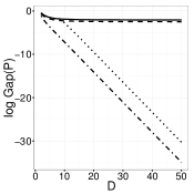
(b) $b=0.5$

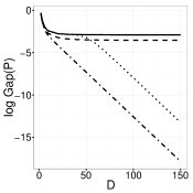
(c) $b=0.9$

Figure 1: Plot of the $\log$ spectral gap against $D$ for $P_{\ref{alg:pm_kernel_2},1}$ (dot-dashed), $P_{\ref{alg:pm_kernel_2},100}$ (dotted), $P_{\ref{alg:1_hit_kernel}}$ (dashed) and $P_{{\rm MH}}$ (solid), with $a=0.5$.

Figures 2 and 3 show $\log{\rm var}(P,\varphi)$ against $D$ for $\varphi_{1}(\theta)=\theta$ and $\varphi_{2}(\theta)=(ab)^{-\theta/2.1}$, respectively, computed using the expression of Kemeny & Snell (1969, p. 84). The choice of $\varphi_{2}$ is motivated by the fact when $p$ is not truncated, $\varphi(\theta)=(ab)^{-\theta/(2+\delta)}$ is in $L^{2}(\pi)$ if and only if $\delta>0$. While ${\rm var}(P,\varphi_{1})$ is stable for all the kernels, ${\rm var}(P,\varphi_{2})$ increases rapidly with $D$ for $P_{\ref{alg:pm_kernel_2},1}$ and $P_{\ref{alg:pm_kernel_2},100}$. While ${\rm var}(P_{\ref{alg:pm_kernel_2},N},\varphi_{1})$ can be lower than ${\rm var}(P_{\ref{alg:1_hit_kernel}},\varphi_{1})$, the former requires many more simulations from the likelihood. Indeed, while the results we have obtained pertain to qualitative properties of the Markov kernels, this example illustrates that $P_{\ref{alg:1_hit_kernel}}$ can significantly outperform $P_{\ref{alg:pm_kernel_2},100}$ for estimating even the more well-behaved $\pi(\varphi_{1})$, when cost per iteration of each kernel is taken into account.

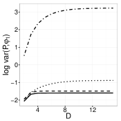
(a) $b=0.1$

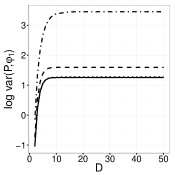
(b) $b=0.5$

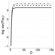
(c) $b=0.9$

Figure 2: Plot of $\log{\rm var}(P,\varphi_{1})$ against $D$ for $P=P_{\ref{alg:pm_kernel_2},1}$ (dot-dashed), $P=P_{\ref{alg:pm_kernel_2},100}$ (dotted), $P=P_{\ref{alg:1_hit_kernel}}$ (dashed) and $P=P_{{\rm MH}}$ (solid), with $a=0.5$.

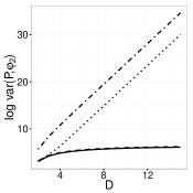
(a) $b=0.1$

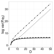
(b) $b=0.5$

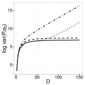
(c) $b=0.9$

Figure 3: Plot of $\log{\rm var}(P,\varphi_{2})$ against $D$ for $P=P_{\ref{alg:pm_kernel_2},1}$ (dot-dashed), $P=P_{\ref{alg:pm_kernel_2},100}$ (dotted), $P=P_{\ref{alg:1_hit_kernel}}$ (dashed) and $P=P_{{\rm MH}}$ (solid), with $a=0.5$.

(a) $b=0.1$

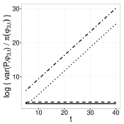
(b) $b=0.5$

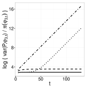
(c) $b=0.9$

Figure 4: Plot of $\log\left\{{\rm var}(P,\varphi_{3,t})/\pi(\varphi_{3,t})\right\}$ against $t$ for $P=P_{\ref{alg:pm_kernel_2},1}$ (dot-dashed), $P=P_{\ref{alg:pm_kernel_2},100}$ (dotted), $P=P_{\ref{alg:1_hit_kernel}}$ (dashed) and $P=P_{{\rm MH}}$ (solid), with $a=0.5$.

Figure 4 shows $\log\left\{{\rm var}(P,\varphi_{3,t})/\pi(\varphi_{3,t})\right\}$ against $t$ for $\varphi_{3,t}(\theta)=\mathbf{1}_{\{t,t+1,\ldots\}}(\theta)$ so that $\pi(\varphi_{3,t})$ is the tail probability. The division by $\pi(\varphi_{3,t})$ makes this an appropriately scaled relative asymptotic variance since one needs $1/\pi(\varphi_{3,t})$ perfect samples from $\pi$ in expectation to get a single sample in the region $\{t,t+1,\ldots\}$. The figure shows that while $P_{{\rm MH}}$ and $P_{\ref{alg:1_hit_kernel}}$ have constant $\log\left\{{\rm var}(P,\varphi_{3,t})/\pi(\varphi_{3,t})\right\}$ as $t$ increases, $P_{\ref{alg:pm_kernel_2},1}$ and $P_{\ref{alg:pm_kernel_2},100}$ do not, as a result of their inability to estimate tail probabilities accurately. In various applications, approximate Bayesian computation might be used to infer such posterior tail probabilities and these results indicate that $P_{\ref{alg:pm_kernel_1},N}$ and $P_{\ref{alg:pm_kernel_2},N}$ may not be appropriate when such inferences are desired.

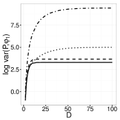
(a) $a=0.9$

(b) $a=0.99$

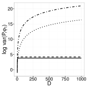
(c) $a=0.999$

Figure 5: Plot of $\log{\rm var}(P,\varphi_{1})$ against $D$ for $P=P_{\ref{alg:pm_kernel_2},1}$ (dot-dashed), $P=P_{\ref{alg:pm_kernel_2},100}$ (dotted), $P=P_{\ref{alg:1_hit_kernel}}$ (dashed) and $P=P_{{\rm MH}}$ (solid), with $b=0.5$.

Figure 5 shows the behaviour of the estimate of the posterior mean for $a\in\{0.9,0.99,0.999\}$ with corresponding values of $n$ for $P_{\ref{alg:1_hit_kernel}}$ being approximately $5$, $50$ and $500$. To take account of the cost of the kernels, it is informative to consider $N{\rm var}(P_{\ref{alg:pm_kernel_2},N},\varphi_{1})$ and $n{\rm var}(P_{\ref{alg:1_hit_kernel}},\varphi_{1})$. For these values of $a$, we have ${\rm var}(P_{\ref{alg:pm_kernel_2},1},\varphi_{1})$ roughly equal to $100{\rm var}(P_{\ref{alg:pm_kernel_2},100},\varphi_{1})$, although $P_{\ref{alg:pm_kernel_2},100}$ is more feasibly implemented in parallel on emerging many-core devices such as graphics processing units (see, e.g., Lee et al., 2010). On the other hand ${\rm var}(P_{\ref{alg:pm_kernel_2},1},\varphi_{1})/\left\{n{\rm var}(P_{\ref{alg:1_hit_kernel}},\varphi_{1})\right\}$ is about $75$, $5000$ and well over $60000$ for $a$ equal to $0.9$, $0.99$ and $0.999$ respectively.

4.3 Stochastic Lotka–Volterra model

We turn to stochastic kinetic models for which the posterior is not of a simple form, and exhibits strong correlations between components of $\theta$. Such models are used, e.g., in systems biology where Bayesian inference has been investigated in Boys et al. (2008) and Wilkinson (2006). We consider a simple member of this class of models, the Lotka–Volterra predator-prey model (Lotka, 1925; Volterra, 1926), which was also considered as an example for approximate Bayesian computation in Toni et al. (2009) and Fearnhead & Prangle (2012).

In this setting $X_{1:2}(t)$ is bivariate, integer-valued pure jump Markov process with $X_{1:2}(0)=(50,100)$. For small $\Delta t$, we have

$${\rm pr}\left\{X_{1:2}(t+\Delta t)=z_{1:2}\mid X_{1:2}(t)=x_{1:2}\right\}\\ =\begin{cases}\theta_{1}x_{1}\Delta t+o(\Delta t)&\text{if }z_{1:2}=(x_{1}+1,x_{2}),\\ \theta_{2}x_{1}x_{2}\Delta t+o(\Delta t)&\text{if }z_{1:2}=(x_{1}-1,x_{2}+1),\\ \theta_{3}x_{2}\Delta t+o(\Delta t)&\text{if }z_{1:2}=(x_{1},x_{2}-1),\\ 1-\Delta t\left(\theta_{1}x_{1}+\theta_{2}x_{1}x_{2}+\theta_{3}x_{2}\right)+o(\Delta t)&\text{if }z_{1:2}=x_{1:2},\\ o(\Delta t)&{\rm otherwise},\end{cases}$$

where the first three cases correspond in order to prey birth, prey consumption and predator death. Theory and methodology related to the simulation of this type of time-homogeneous, pure jump Markov process and historical uses in statistics can be traced through Feller (1940), Doob (1945) and Kendall (1949, 1950), and the method was rediscovered in Gillespie (1977) in the context of stochastic kinetic models. These articles develop a straightforward way to simulate the full process $X_{1:2}(t),\;t\in[0,10]$, as the inter-jump times are exponential random variables, although more sophisticated approaches are possible (see, e.g., Wilkinson, 2006, Chapter 8).

The data was simulated with $\theta=(1,0.005,0.6)$, an example from Wilkinson (2006, p. 152). Our observations are both partial and discrete with $y=\{88,165,274,268,114,46,32,36,53,92\}$ the simulated values of $X_{1}$ at times $\{1,2,\ldots,10\}$, and for approximate Bayesian computation we use a $\log$ transformation of $X_{1}(t)$ and $y(t)$ with $\epsilon=1$, i.e.,

$$B_{\epsilon}(y)=\left\{X_{1}(t)\;:\;\log\left\{X_{1}(i)\right\}-\log\left\{y(i)\right\}\leq\epsilon,\text{ for each }i\in\{1,\ldots,10\}\right\}.$$

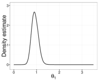
(a)

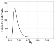
(b)

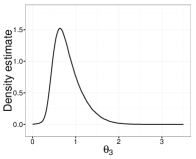
(c)

Figure 6: Density estimates of the marginal posteriors for the Lotka–Volterra model.

(a) $P_{\ref{alg:pm_kernel_1},1}$

(b) $P_{\ref{alg:pm_kernel_1},15}$

(c) $P_{\ref{alg:pm_kernel_2},15}$

(d) $P_{\ref{alg:1_hit_kernel}}$

Figure 7: Estimates of the posterior mean of $\theta_{3}$ by iteration using each kernel. The three horizontal lines correspond to the estimate obtained using the rejection sampler with two estimated standard deviations added and subtracted.

(a) $P_{\ref{alg:pm_kernel_1},1}$

(b) $P_{\ref{alg:pm_kernel_1},15}$

(c) $P_{\ref{alg:pm_kernel_2},15}$

(d) $P_{\ref{alg:1_hit_kernel}}$

Figure 8: Estimates of $\pi(\theta_{3}\geq 1.79)$ by iteration using each kernel. The three horizontal lines correspond to the estimate obtained using the rejection sampler with two estimated standard deviations added and subtracted.

We first model $\theta\in\Theta=[0,\infty)^{3}$ with $p(\theta)=100\exp(-\theta_{1}-100\theta_{2}-\theta_{3})$ and use $q(\theta,\vartheta)=\mathcal{N}(\vartheta;\theta,\Sigma)$ where $\Sigma={\rm diag}(.25,0.0025,.25)$. The choice of independent exponential priors on $\theta$ is motivated by Condition 2. Density plots of the marginal posteriors for each component of $\theta$ are shown in Figure 6, obtained using $10^{6}$ samples from $\pi$ using a rejection sampler. $\theta_{1}$ has a tighter posterior than $\theta_{3}$ and while not shown here, the samples indicate strong positive correlation between $\theta_{2}$ and $\theta_{3}$. In this setting, $P_{\ref{alg:1_hit_kernel}}$ for $5\times 10^{6}$ iterations gave an average value of $n$ of $15$ and we also ran kernels $P_{\ref{alg:pm_kernel_1},1}=P_{\ref{alg:pm_kernel_2},1}$ for $5\times 10^{7}$ iterations and $P_{\ref{alg:pm_kernel_1},15}$ and $P_{\ref{alg:pm_kernel_2},15}$ both for $5\times 10^{6}$ iterations. All kernels gave density estimates visibly indistinguishable from those in Figure 6, but inspection of their partial sums by iteration reveals important differences. In Figures 7 and 8 we show estimates of the posterior mean of $\theta_{3}$ and the probability that $\theta_{3}\geq 1.79$ for each chain, accompanied by lines corresponding to the estimate obtained using the samples from the rejection sampler. The choice of $1.79$ corresponds to an estimate of the 90th percentile using these latter samples. $P_{\ref{alg:1_hit_kernel}}$ seems to accurately estimate both the same value as the estimate from the rejection sampler and the uncertainty of the estimate seems to be correlated with perturbations of the partial sum. However, the other kernels seem to both miss the value of interest by some amount and, particularly in the case of $P_{\ref{alg:pm_kernel_1},1}$, the perturbations of the partial sum over time are small which may mislead practitioners into believing the estimate has converged.

We performed a second analysis using a slightly different prior, with $p(\theta)=0.01\exp(-\theta_{1}-0.01\theta_{2}-\theta_{3})$, where differences in the kernels are accentuated. Here, the independent prior for $\theta_{2}$ is all that has changed, and has been made less informative. In this case, a rejection sampler cannot practically be used to verify results as the expected number of proposals required to obtain one sample by rejection is around $4.5\times 10^{5}$. The average value of $n$ for $P_{\ref{alg:1_hit_kernel}}$, however, was $13$.

(a) $P_{\ref{alg:pm_kernel_1},1}$

(b) $P_{\ref{alg:pm_kernel_1},15}$

(c) $P_{\ref{alg:pm_kernel_2},15}$

(d) $P_{\ref{alg:1_hit_kernel}}$

Figure 9: Estimates of the posterior mean of $\theta_{2}$ by iteration using each kernel.

(a) $P_{\ref{alg:pm_kernel_1},1}$

(b) $P_{\ref{alg:pm_kernel_1},15}$

(c) $P_{\ref{alg:pm_kernel_2},15}$

(d) $P_{\ref{alg:1_hit_kernel}}$

Figure 10: Estimates of $\pi(\theta_{3}\geq 2)$ by iteration using each kernel.

While not shown here, marginal posterior density estimates using each kernel for the parameters are reasonably close to those in Figure 6, but those corresponding to $P_{\ref{alg:pm_kernel_1},1}$ exhibit characteristic ‘bumps’ in its tail. As above, we can inspect each chain’s corresponding partial sums by iteration to reveal important differences. Figures 9 and 10 show estimates of the posterior mean of $\theta_{2}$ and the posterior probability that $\theta_{3}\geq 2$ for each chain respectively, and the latter is particularly illustrative of the inability of $P_{\ref{alg:pm_kernel_1}}$ and $P_{\ref{alg:pm_kernel_2}}$ to produce chains without long tail excursions.

In practical applications such as this, it may not be possible to determine easily if $P_{{\rm MH}}$ is variance bounding or geometrically ergodic. However, Theorems 3–4 do establish that $P_{\ref{alg:1_hit_kernel}}$ will inherit either of these properties from $P_{{\rm MH}}$ if it is. In practice, it is not unusual for the conditions of Corollary 1 to hold, and one might expect them to do so here. Similarly, it is also quite common for Condition 1 to hold, and so one might expect that $P_{\ref{alg:pm_kernel_1}}$ and $P_{\ref{alg:pm_kernel_2}}$ are not variance bounding here.

5 Discussion

Our analysis suggests that $P_{\ref{alg:1_hit_kernel}}$ may be geometrically ergodic and/or variance bounding in a wide variety of situations where kernels $P_{\ref{alg:pm_kernel_1},N}$ and $P_{\ref{alg:pm_kernel_2},N}$ are not. In practice, Condition 2 can be verified and used to inform prior and proposal choice to ensure that $P_{\ref{alg:1_hit_kernel}}$ systematically inherits these properties from $P_{{\rm MH}}$. Of course, variance bounding or geometric ergodicity of $P_{{\rm MH}}$ is often impossible to verify in the approximate Bayesian computation setting due to the unknown nature of $f_{\theta}$. However, a prior with regular contours as per (11) will ensure that $P_{{\rm MH}}$ is geometrically ergodic if $f_{\theta}$ decays super-exponentially and also has regular contours. In addition, Condition 2 is stronger than necessary but tighter conditions are likely to be complicated and may require case-by-case treatment.

The combination of Theorems 2–3 and Proposition 3, whose assumptions are not mutually exclusive, allow us to conclude that the behaviour of $P_{\ref{alg:1_hit_kernel}}$ is characteristically different to $P_{\ref{alg:pm_kernel_1},N}$ and $P_{\ref{alg:pm_kernel_2},N}$ in some settings. In particular, the use of a larger expected number of simulations from $f_{\theta}$ and $f_{\vartheta}$ in the tails of $\pi$ using $P_{\ref{alg:1_hit_kernel}}$ could be viewed as analogous to being “stuck” for many iterations in the tails of $\pi$ using $P_{\ref{alg:1_hit_kernel}}$ or $P_{\ref{alg:pm_kernel_2},N}$. However, while both the expected number of simulations and the asymptotic variance of (3) for any $\varphi\in L^{2}(\pi)$ are finite under $P_{\ref{alg:1_hit_kernel}}$ under the conditions of Theorem 3, there are $\varphi\in L^{2}(\pi)$ for which a central limit theorem does not hold for (3) when using $P_{\ref{alg:pm_kernel_1},N}$ or $P_{\ref{alg:pm_kernel_2},N}$ under the conditions of Theorem 2.

Variance bounding and geometric ergodicity are likely to coincide in most applications of interest, as variance bounding but non-geometrically ergodic Metropolis–Hastings kernels exhibit periodic behaviour rarely encountered in statistical inference. Bounds on the second largest eigenvalue and/or spectral gap of $P_{\ref{alg:1_hit_kernel}}$ in relation to properties of $P_{{\rm MH}}$ could be obtained through Cheeger-like inequalities using conductance arguments as in the proofs of Theorems 3 and 4, although these may be quite loose in some situations (see, e.g., Diaconis & Stroock, 1991) and we have not pursued them here. Finally, Roberts & Rosenthal (2011) have demonstrated that some simple Markov chains that are not geometrically ergodic can converge extremely slowly and that properties of such algorithms can be very sensitive to even slight parameter changes.

The theoretical results obtained in Section 3 and the examples in Section 4 provide some understanding of the relative qualitative merits of $P_{\ref{alg:1_hit_kernel}}$ over $P_{\ref{alg:pm_kernel_1},N}$ and $P_{\ref{alg:pm_kernel_2},N}$. However, the results do not prove that $P_{\ref{alg:1_hit_kernel}}$ should necessarily be uniformly preferred over $P_{\ref{alg:pm_kernel_2},N}$, although the examples do suggest that it may have better asymptotic variance properties when taking cost of simulations into account in a variety of scenarios. In addition, Theorem 5 can be used to justify its mixture with alternative reversible kernels such as $P_{\ref{alg:pm_kernel_2},N}$ if desired.

Appendix A Proofs

Many of our proofs make use of the relationship between conductance, the spectrum of a Markov kernel, and variance bounding for reversible Markov kernels $P$. In particular, conductance $\kappa>0$ is equivalent to $\sup S(P)<1$ (Lawler & Sokal, 1988, Theorem 2.1), which as stated earlier is equivalent to variance bounding. Conductance $\kappa$ for a $\pi$-invariant, transition kernel $P$ on $\Theta$ is defined as

$$\kappa=\inf_{A:0<\pi(A)\leq 1/2}\kappa(A),\qquad\kappa(A)=\pi(A)^{-1}\int_{A}P(\theta,A^{\complement})\pi(\mathrm{d}\theta)=\int_{\Theta}P(\theta,A^{\complement})\pi_{A}(\mathrm{d}\theta),$$

where $\pi_{A}(\mathrm{d}\theta)=\pi(\mathrm{d}\theta)\mathbf{1}_{A}(\theta)/\pi(A)$.

Finally, we make use of the fact that if $q\in\mathcal{Q}$ we can define the function

$$r_{q}(\delta)=\inf\left\{r:\text{ for all }\theta\in\Theta,\;q\left(\theta,B_{r,\theta}^{\complement}\right)<\delta\right\}.$$

Proof of Theorem 1.

If $\nu-{\rm ess}\sup_{\theta}P(\theta,\{\theta\})=1$ and $P(\theta,\{\theta\})$ is measurable, then the set $A_{\tau}=\{\theta\in\Theta\,:\,P(\theta,\{\theta\})\geq 1-\tau\}$ is measurable and $\nu(A_{\tau})>0$ for every $\tau>0$. Moreover, $a_{0}=\lim_{\tau\searrow 0}\nu(A_{\tau})$ exists, since $A_{\tau_{2}}\subset A_{\tau_{1}}$ for $\tau_{2}<\tau_{1}$. Now, assume $a_{0}>0$, and define $A_{0}=\{\theta\in\Theta\>:\>P(\theta,\{\theta\})=1\}=\bigcap_{n}A_{\tau_{n}}$ where $\tau_{n}\searrow 0$. By continuity from above $\nu(A_{0})=a_{0}>0$ and since $\nu$ is not concentrated at a single point, $P$ is reducible, which is a contradiction. Hence $a_{0}=0$. Consequently, by taking $\tau_{n}\searrow 0$ with $\tau_{1}$ small enough, we have $\nu(A_{\tau_{n}})<1/2$ for every $n$, and can upper bound the conductance of $P$ by

$$\kappa\leq\lim_{n}\kappa(A_{\tau_{n}})=\lim_{n}\int_{A_{\tau_{n}}}P(\theta,A_{\tau_{n}}^{\complement})\nu_{A_{\tau_{n}}}(\mathrm{d}\theta)\leq\lim_{n}\int_{A_{\tau_{n}}}P(\theta,\{\theta\}^{\complement})\nu_{A_{\tau_{n}}}(\mathrm{d}\theta)=\lim_{n}\tau_{n}=0.$$

Therefore $P\notin\mathcal{V}$. ∎

Proof of Theorem 2.

We prove the result for $P_{\ref{alg:pm_kernel_2},N}$. The proof for $P_{\ref{alg:pm_kernel_1},N}$ is essentially identical, with minor adjustments for the extended state space, and is omitted. By Theorem 1, it suffices to show that $\pi-{\rm ess}\sup_{\theta}P_{\ref{alg:pm_kernel_2},N}(\theta,\{\theta\})=1$, i.e., for all $\tau>0$, there exists $A\subseteq\Theta$ with $\pi(A)>0$ such that for all $\theta\in A$, $P_{\ref{alg:pm_kernel_2},N}(\theta,\{\theta\}^{\complement})\leq\tau$.

From Condition 1, $q\in\mathcal{Q}$. Given $\tau>0$, let $r=r_{q}(\tau/2)$, $v=\inf\left\{v:\sup_{\theta\in B_{v}^{c}(0)}h(\theta)<1-\left(1-\tau/2\right){}^{1/N}\right\}$ and $A=B_{v+r,0}^{\complement}$. From Condition 1, $\pi(A)>0$ and using (5) and (6), for all $\theta\in A$,

$$P_{\ref{alg:pm_kernel_2},N}(\theta,\{\theta\}^{\complement}) =\int_{\{\theta\}^{\complement}}\int_{\mathsf{Y}^{N}}\int_{\mathsf{Y}^{N-1}}\left[1\wedge\frac{c(\vartheta,\theta)\sum_{j=1}^{N}w(z_{j})}{c(\theta,\vartheta)\left\{1+\sum_{j=1}^{N-1}w(x_{j})\right\}}\right]f_{\theta}^{\otimes N-1}({\rm d}x_{1:N-1})f_{\vartheta}^{\otimes N}({\rm d}z_{1:N})q(\theta,{\rm d}\vartheta)$$

$$\leq\sup_{\theta\in\Theta}q\left(\theta,B_{r,\theta}^{\complement}\right)+\int_{B_{r,\theta}}\int_{\mathsf{Y}^{N}}I\left\{\sum_{i=1}^{N}w(z_{i})\geq 1\right\}f_{\vartheta}^{\otimes N}({\rm d}z_{1:N})q(\theta,{\rm d}\vartheta)$$

$$\leq\frac{\tau}{2}+\int_{B_{r,\theta}}\left[1-\left\{1-\sup_{\vartheta\in B_{r,\theta}}h(\vartheta)\right\}^{N}\right]q(\theta,{\rm d}\vartheta)\leq\tau.$$

∎

The following two Lemmas are pivotal in the proofs of Proposition 1 and Theorems 3 and 4, and make extensive use of (5), (7) and (8). Their proofs can be found in Appendix B.

Lemma 1.

$P_{\ref{alg:1_hit_kernel}}(\theta,\{\theta\})\geq P_{{\rm MH}}(\theta,\{\theta\})$.

Lemma 2.

Assume Condition 2. For $\pi$-almost all $\theta$ and any $A\subseteq\Theta$ such that $\theta\in A$ and $r>0$,

$$P_{{\rm MH}}(\theta,A^{\complement})\leq\sup_{\theta}q(\theta,B_{r,\theta}^{\complement})+(1+M_{r})P_{\ref{alg:1_hit_kernel}}(\theta,A^{\complement}),$$

where $M_{r}$ is as defined in Condition 2.

Proof of Theorem 3.

We prove the result under Condition 2. Let $\kappa_{{\rm MH}}$ and $\kappa_{\ref{alg:1_hit_kernel}}$ be the conductance of $P_{{\rm MH}}$ and $P_{\ref{alg:1_hit_kernel}}$ respectively, and $A$ be a measurable set with $\pi(A)>0$. Since $q\in\mathcal{Q}$ we let $R=r_{q}(\kappa_{{\rm MH}}/2)$ and $M_{R}$ be as in Condition 2. Then by Lemma 2 we have

$$\kappa_{{\rm MH}}(A) =\int_{\Theta}P_{{\rm MH}}(\theta,A^{\complement})\pi_{A}(\mathrm{d}\theta)\leq\frac{\kappa_{{\rm MH}}}{2}+(1+M_{R})\int_{\Theta}P_{\ref{alg:1_hit_kernel}}(\theta,A^{\complement})\pi_{A}(\mathrm{d}\theta)$$

$$=\frac{\kappa_{{\rm MH}}}{2}+(1+M_{R})\kappa_{\ref{alg:1_hit_kernel}}(A).$$

Since $A$ is arbitrary, we conclude that $\kappa_{{\rm MH}}\leq 2(1+M_{R})\kappa_{\ref{alg:1_hit_kernel}}$ so $\kappa_{{\rm MH}}>0\Rightarrow\kappa_{\ref{alg:1_hit_kernel}}>0$. ∎

Appendix B Supplementary proofs

Proof of Proposition 1.

Lemma 1 gives $P_{\ref{alg:1_hit_kernel}}\preceq P_{{\rm MH}}$ in the sense of (Peskun, 1973; Tierney, 1998) and so ${\rm var}(P_{\ref{alg:1_hit_kernel}},\varphi)\geq{\rm var}(P_{{\rm MH}},\varphi)$. By Roberts & Rosenthal (2008, Theorem 8), $P_{\ref{alg:1_hit_kernel}}\preceq P_{{\rm MH}}\Longrightarrow(P_{\ref{alg:1_hit_kernel}}\in\mathcal{V}\Rightarrow P_{{\rm MH}}\in\mathcal{V})$. ∎

Proof of Lemma 1.

We show that for any $(\theta,\vartheta)$, $\alpha_{\ref{alg:1_hit_kernel}}(\theta,\vartheta)\leq\alpha_{{\rm MH}}(\theta,\vartheta)$. Consider the case $c(\vartheta,\theta)\leq c(\theta,\vartheta)$. Then since $h(\theta)\leq 1$,

$$\alpha_{\ref{alg:1_hit_kernel}}(\theta,\vartheta) =\frac{c(\vartheta,\theta)}{c(\theta,\vartheta)}\frac{h(\vartheta)}{h(\vartheta)+h(\theta)-h(\vartheta)h(\theta)}\leq 1\wedge\frac{c(\vartheta,\theta)h(\vartheta)}{c(\theta,\vartheta)h(\theta)}=\alpha_{{\rm MH}}(\theta,\vartheta).$$

Similarly, if $c(\vartheta,\theta)>c(\theta,\vartheta)$, we have

$$\alpha_{\ref{alg:1_hit_kernel}}(\theta,\vartheta)=\frac{h(\vartheta)}{h(\vartheta)+h(\theta)-h(\vartheta)h(\theta)}\leq 1\wedge\frac{c(\vartheta,\theta)h(\vartheta)}{c(\theta,\vartheta)h(\theta)}=\alpha_{{\rm MH}}(\theta,\vartheta).$$

This immediately implies $P_{\ref{alg:1_hit_kernel}}(\theta,\{\theta\})\geq P_{{\rm MH}}(\theta,\{\theta\})$ since $P(\theta,\{\theta\})=1-\int_{\Theta\setminus\{\theta\}}q(\theta,\vartheta)\alpha(\theta,\vartheta)d\vartheta$. ∎

Proof of Lemma 2.

We begin by showing that for $\vartheta\in B_{r}(\theta)$ and $\vartheta\neq\theta$,

$$\alpha_{{\rm MH}}(\theta,\vartheta) \leq(1+M_{r})\alpha_{\ref{alg:1_hit_kernel}}(\theta,\vartheta).$$ (13)

First we deal with the case $h(\vartheta)p(\vartheta)q(\vartheta,\theta)=0$. Then the inequality is trivially satisfied as $\alpha_{{\rm MH}}(\theta,\vartheta)=\alpha_{\ref{alg:1_hit_kernel}}(\theta,\vartheta)=0$. Conversely, if $\pi(\theta)q(\theta,\vartheta)>0$ and $\pi(\vartheta)q(\vartheta,\theta)>0$ and additionally $\vartheta\in B_{r,\theta}$, then under Condition 2,

$$\frac{(1+M_{r})c(\vartheta,\theta)h(\vartheta)}{\alpha_{{\rm MH}}(\theta,\vartheta)} =(1+M_{r})\left\{c(\theta,\vartheta)h(\theta)\vee c(\vartheta,\theta)h(\vartheta)\right\}$$

$$\geq\left\{c(\theta,\vartheta)h(\theta)\vee c(\vartheta,\theta)h(\vartheta)\right\}+\left\{c(\theta,\vartheta)h(\vartheta)\vee c(\vartheta,\theta)h(\theta)\right\}$$

$$\geq\{(c(\theta,\vartheta)h(\theta)+c(\theta,\vartheta)h(\vartheta))\vee(c(\vartheta,\theta)h(\vartheta)+c(\vartheta,\theta)h(\theta))\}$$

$$=\frac{c(\vartheta,\theta)h(\vartheta)}{\{\frac{c(\vartheta,\theta)h(\vartheta)}{c(\theta,\vartheta)h(\theta)+c(\theta,\vartheta)h(\vartheta)}\wedge\frac{c(\vartheta,\theta)h(\vartheta)}{c(\vartheta,\theta)h(\vartheta)+c(\vartheta,\theta)h(\theta)}\}}=\frac{c(\vartheta,\theta)h(\vartheta)}{\frac{h(\vartheta)}{h(\vartheta)+h(\theta)}\{\frac{c(\vartheta,\theta)}{c(\theta,\vartheta)}\wedge 1\}}$$

$$\geq\frac{c(\vartheta,\theta)h(\vartheta)}{\alpha_{\ref{alg:1_hit_kernel}}(\theta,\vartheta)},$$

i.e., $\alpha_{{\rm MH}}(\theta,\vartheta)\leq(1+M_{r})\alpha_{\ref{alg:1_hit_kernel}}(\theta,\vartheta)$. The first inequality is obtained by recalling that under Condition 2, when $\pi(\theta)q(\theta,\vartheta)\wedge\pi(\vartheta)q(\vartheta,\theta)>0$ we have $M_{r}^{-1}\leq h(\vartheta)/h(\theta)\leq M_{r}$ or $M_{r}^{-1}\leq c(\vartheta,\theta)/c(\theta,\vartheta)\leq M_{r}$ and in either case $M_{r}\left\{c(\theta,\vartheta)h(\theta)\vee c(\vartheta,\theta)h(\vartheta)\right\}\geq\left\{c(\theta,\vartheta)h(\vartheta)\right\}\vee\left\{c(\vartheta,\theta)h(\theta)\right\}$.

Hence, we have

$$P_{{\rm MH}}(\theta,A^{\complement}) =\int_{A^{\complement}}\alpha_{{\rm MH}}(\theta,\vartheta)q(\theta,{\rm d}\vartheta)\leq q(\theta,B_{r,\theta}^{\complement})+\int_{A^{\complement}\cap B_{r,\theta}}(1+M_{r})\alpha_{\ref{alg:1_hit_kernel}}(\theta,\vartheta)q(\theta,{\rm d}\vartheta)$$

$$\leq\sup_{\theta}q(\theta,B_{r,\theta}^{\complement})+(1+M_{r})P_{\ref{alg:1_hit_kernel}}(\theta,A^{\complement}).$$

∎

Proof of Theorem 4.

Recall that geometric ergodicity is equivalent to $\sup|\sigma_{0}(P)|<1$. From the spectral mapping theorem (Conway, 1990) this is equivalent to $\sup\sigma_{0}(P^{2})<1$, where $\sigma_{0}(P^{2})$ is the spectrum of $P^{2}$, the two-fold iterate of $P$. We denote by $\kappa_{\ref{alg:1_hit_kernel}}^{(2)}$ and $\kappa_{{\rm MH}}^{(2)}$ the conductance of $P_{\ref{alg:1_hit_kernel}}^{2}$ and $P_{{\rm MH}}^{2}$ respectively. Since $q\in\mathcal{Q}$ we let $R=r_{q}(\kappa_{{\rm MH}}^{(2)}/4)$ and $M_{R}$ be as in Condition 2. By Lemmas 1 and 2, we have for any measurable $A\subseteq\Theta$

$$P_{{\rm MH}}(\theta,A) =P_{{\rm MH}}(\theta,A\setminus\{\theta\})+I(\theta\in A)P_{{\rm MH}}(\theta,\{\theta\})$$

$$\leq\kappa_{{\rm MH}}^{(2)}/4+(1+M_{R})P_{\ref{alg:1_hit_kernel}}(\theta,A\setminus\{\theta\})+P_{\ref{alg:1_hit_kernel}}(\theta,\{\theta\})$$

$$\leq\kappa_{{\rm MH}}^{(2)}/4+(1+M_{R})P_{\ref{alg:1_hit_kernel}}(\theta,A).$$

We can also upper bound, for any $\theta\in\Theta$, the Radon–Nikodym derivative of $P_{{\rm MH}}(\theta,\cdot)$ with respect to $P_{\ref{alg:1_hit_kernel}}(\theta,\cdot)$ for any $\vartheta\in B_{R,\theta}$ as

$$\frac{{\rm d}P_{{\rm MH}}(\theta,\cdot)}{{\rm d}P_{\ref{alg:1_hit_kernel}}(\theta,\cdot)}(\vartheta) =I(\vartheta\in B_{R,\theta}\setminus\{\theta\})\frac{{\rm d}q(\theta,\cdot)}{{\rm d}q(\theta,\cdot)}(\vartheta)\frac{\alpha_{{\rm MH}}(\theta,\vartheta)}{\alpha_{\ref{alg:1_hit_kernel}}(\theta,\vartheta)}+I(\vartheta=\theta)\frac{P_{{\rm MH}}(\theta,\{\theta\})}{P_{\ref{alg:1_hit_kernel}}(\theta,\{\theta\})}$$

$$\leq I(\vartheta\in B_{R,\theta}\setminus\{\theta\})(1+M_{R})+I(\vartheta=\theta)\leq 1+M_{R},$$

where we have used (13) and Lemma 1 in the first inequality.

Let $A$ be a measurable set with $\pi(A)>0$. We have

$$\kappa_{{\rm MH}}^{(2)}(A) =\int_{A}\left\{\int_{\Theta}P_{{\rm MH}}(\vartheta,A^{\complement})P_{{\rm MH}}(\theta,{\rm d}\vartheta)\right\}\pi_{A}(\mathrm{d}\theta)$$

$$=\int_{A}\left\{\int_{B_{R,\theta}^{\complement}}P_{{\rm MH}}(\vartheta,A^{\complement})P_{{\rm MH}}(\theta,{\rm d}\vartheta)+\int_{B_{R,\theta}}P_{{\rm MH}}(\vartheta,A^{\complement})P_{{\rm MH}}(\theta,{\rm d}\vartheta)\right\}\pi_{A}(\mathrm{d}\theta)$$

$$\leq\int_{A}\left\{q(\theta,B_{R,\theta}^{\complement})+\int_{B_{R,\theta}}P_{{\rm MH}}(\vartheta,A^{\complement})P_{{\rm MH}}(\theta,{\rm d}\vartheta)\right\}\pi_{A}(\mathrm{d}\theta)$$

$$\leq\kappa_{{\rm MH}}^{(2)}/4+\int_{A}\int_{B_{R,\theta}}P_{{\rm MH}}(\vartheta,A^{\complement})P_{{\rm MH}}(\theta,{\rm d}\vartheta)\pi_{A}(\mathrm{d}\theta)$$

$$\leq\kappa_{{\rm MH}}^{(2)}/4+\int_{A}\int_{B_{R,\theta}}\left\{\kappa_{{\rm MH}}^{(2)}/4+(1+M_{R})P_{\ref{alg:1_hit_kernel}}(\vartheta,A^{\complement})\right\}P_{{\rm MH}}(\theta,{\rm d}\vartheta)\pi_{A}(\mathrm{d}\theta)$$

$$\leq\kappa_{{\rm MH}}^{(2)}/2+(1+M_{R})\int_{A}\int_{B_{R,\theta}}P_{\ref{alg:1_hit_kernel}}(\vartheta,A^{\complement})P_{{\rm MH}}(\theta,{\rm d}\vartheta)\pi_{A}(\mathrm{d}\theta)$$

$$=\kappa_{{\rm MH}}^{(2)}/2+(1+M_{R})\int_{A}\int_{B_{R,\theta}}P_{\ref{alg:1_hit_kernel}}(\vartheta,A^{\complement})\frac{{\rm d}P_{{\rm MH}}(\theta,\cdot)}{{\rm d}P_{\ref{alg:1_hit_kernel}}(\theta,\cdot)}(\vartheta)P_{\ref{alg:1_hit_kernel}}(\theta,{\rm d}\vartheta)\pi_{A}(\mathrm{d}\theta)$$

$$\leq\kappa_{{\rm MH}}^{(2)}/2+(1+M_{R})^{2}\int_{A}\int_{B_{R,\theta}}P_{\ref{alg:1_hit_kernel}}(\vartheta,A^{\complement})P_{\ref{alg:1_hit_kernel}}(\theta,{\rm d}\vartheta)\pi_{A}(\mathrm{d}\theta)$$

$$\leq\kappa_{{\rm MH}}^{(2)}/2+(1+M_{R})^{2}\int_{A}\int_{\Theta}P_{\ref{alg:1_hit_kernel}}(\vartheta,A^{\complement})P_{\ref{alg:1_hit_kernel}}(\theta,{\rm d}\vartheta)\pi_{A}(\mathrm{d}\theta)$$

$$=\kappa_{{\rm MH}}^{(2)}/2+(1+M_{R})^{2}\kappa_{\ref{alg:1_hit_kernel}}^{(2)}(A).$$

Since $A$ is arbitrary, we conclude that $\kappa_{{\rm MH}}^{(2)}\leq 2(1+M_{R})^{2}\kappa_{\ref{alg:1_hit_kernel}}^{(2)}$ so $\kappa_{{\rm MH}}^{(2)}>0\Rightarrow\kappa_{\ref{alg:1_hit_kernel}}^{(2)}>0$.∎

Lemma 3.

Let $K_{1}$ be a reversible Markov kernel with unique invariant distribution $\pi$ and let $K_{2}$ be reversible with invariant distribution $\pi$. Let $\tilde{K}=aK_{1}+(1-a)K_{2}$ be a mixture of $K_{1}$ and $K_{2}$ for $a\in(0,1]$. Then $K_{1}\in\mathcal{V}\Rightarrow\tilde{K}\in\mathcal{V}$ and $K_{1}\in\mathcal{G}\Rightarrow\tilde{K}\in\mathcal{G}$.

Proof.

For the first part, assume $K_{1}\in\mathcal{V}$. Then since $K_{1}$ is reversible with unique invariant distribution $\pi$, its conductance $\kappa_{1}$ satisfies $\kappa_{1}>0$. Since $K_{2}$ is also reversible, the mixture $\tilde{K}$ is reversible with unique invariant distribution $\pi$ and its conductance is

$$\tilde{\kappa} =\inf_{A:0<\pi(A)\leq 1/2}\int_{A}\tilde{K}(\theta,A^{\complement})\pi_{A}(\mathrm{d}\theta)$$

$$\geq\inf_{A:0<\pi(A)\leq 1/2}\int_{A}aK_{1}(\theta,A^{\complement})\pi_{A}(\mathrm{d}\theta)$$

$$=a\kappa_{1}>0.$$

Hence $\tilde{K}\in\mathcal{V}$.

Similarly, for the second part, assume $K_{1}\in\mathcal{G}$. Then the conductance of $K_{1}^{2}$, $\kappa_{1}^{(2)}$, satisfies $\kappa_{1}^{(2)}>0$ by the spectral mapping theorem (Conway, 1990). Let $\tilde{\kappa}^{(2)}$ be the conductance of $\tilde{K}^{2}$, and it suffices to show that $\tilde{\kappa}^{(2)}>0$. We have

$$\tilde{\kappa}^{(2)} =\inf_{A:0<\pi(A)\leq 1/2}\int_{A}\tilde{K}^{2}(\theta,A^{\complement})\pi_{A}(\mathrm{d}\theta)$$

$$\geq\inf_{A:0<\pi(A)\leq 1/2}\int_{A}a^{2}K_{1}^{2}(\theta,A^{\complement})\pi_{A}(\mathrm{d}\theta)$$

$$=a^{2}\kappa_{1}^{(2)}>0.$$

Hence $\tilde{K}\in\mathcal{G}$. ∎

Proof of Theorem 5.

The result is immediate upon defining $L_{1}=K_{1}$, $L_{2}=\left(1-a_{1}\right)^{-1}\sum_{i=2}^{\infty}a_{i}K_{i}$ and $\tilde{L}=a_{1}L_{1}+(1-a_{1})L_{2}$ and applying Lemma 3. ∎

Proof of Proposition 3.

If the current state of the Markov chain is $\theta$, the expected value of $N$ is

$$n(\theta)=\int_{\Theta}\frac{\left[1\wedge\left\{c(\vartheta,\theta)/c(\theta,\vartheta)\right\}\right]}{h(\theta)+h(\vartheta)-h(\theta)h(\vartheta)}q(\theta,{\rm d}\vartheta),$$

since upon drawing $\vartheta\sim q(\theta,\cdot)$, $N=0$ with probability $1-\left\{1\wedge c(\vartheta,\theta)\right\}$ and with probability $\left\{1\wedge c(\vartheta,\theta)\right\}$ it is the minimum of two geometric random variables with success probabilities $h(\theta)$ and $h(\vartheta)$, i.e. it is a geometric random variable with success probability $h(\theta)+h(\vartheta)-h(\theta)h(\vartheta)$.

Since $P_{\ref{alg:1_hit_kernel}}$ is $\pi$-invariant and irreducible, the strong law of large numbers for Markov chains implies

$$n=\int_{\Theta}n(\theta)\pi(\mathrm{d}\theta)=H^{-1}\int_{\Theta^{2}}\frac{\left[1\wedge\left\{c(\vartheta,\theta)/c(\theta,\vartheta)\right\}\right]h(\theta)}{h(\theta)+h(\vartheta)-h(\theta)h(\vartheta)}q(\theta,{\rm d}\vartheta)p({\rm d}\theta)\leq H^{-1}<\infty,$$

where we have used $\int_{\Theta}p(\theta)\mathrm{d}\theta=1$ in the first inequality. ∎

Appendix C Negative results in other settings

This appendix extends Theorem 2 to a number of related approximate Bayesian computation settings. These results indicate that the conclusions of Theorem 2 about lack of geometric ergodicity and variance bounding property hold much more universally. We first consider the case where one utilizes a proposal that falls just outside the definition of $\mathcal{Q}$. Of particular interest could be those proposals that are biased towards the centre of $\Theta$ but are not global. To this end, we can define

$$\mathcal{Q}_{0}=\{q\,:\,\text{for all }\delta>0\>\text{and }r>0,\>\text{there exists }R>0\>\text{such that for all }\theta\in B_{R,0}^{\complement},\>q(\theta,B_{r,0})<\delta\},$$

which includes, for example, the autoregressive proposal $q(\theta,\vartheta)=\mathcal{N}(\vartheta;\rho\theta,\sigma^{2})$ for some $\rho\in(0,1)$. The following result indicates that such proposals are similarly associated with lack of variance bounding for $P_{\ref{alg:pm_kernel_2},N}$.

Proposition 4.

Let $q\in\mathcal{Q}_{0}$ and assume that for all $r>0$, $\pi(B_{r,0}^{\complement})>0$, and for all $\delta>0$ there exists $v>0$ such that $\sup_{\theta\in B_{v,0}^{\complement}}h(\theta)<\delta$. Then $P_{\ref{alg:pm_kernel_2},N}\notin\mathcal{V}$ for any $N\in\mathbb{N}$.

Proof.

By Theorem 1, it suffices to show that $\pi-{\rm ess}\sup_{\theta}P_{\ref{alg:pm_kernel_2},N}(\theta,\{\theta\})=1$. Let $q\in\mathcal{Q}_{0}$, $\tau>0$ and take $r=\inf\left\{r:\sup_{\theta\in B_{r,0}^{\complement}}h(\theta)<1-\left(1-\tau/2\right)^{1/N}\right\}$ and $R=\inf\left\{R:\sup_{\theta\in B_{R,0}^{\complement}}q(\theta,B_{r,0})<\tau/2\right\}$, which both exist by assumption. Furthermore, $\pi(B_{R,0}^{\complement})>0$. Let $A_{\tau}=B_{R,0}^{\complement}$. We have for all $\theta\in A$,

$$P_{\ref{alg:pm_kernel_2},N}(\theta,\{\theta\}^{\complement}) =\int_{\{\theta\}^{\complement}}\int_{\mathsf{Y}^{N}}\int_{\mathsf{Y}^{N-1}}\left[1\wedge\frac{c(\vartheta,\theta)\sum_{j=1}^{N}w(z_{j})}{c(\theta,\vartheta)\left\{1+\sum_{j=1}^{N-1}w(x_{j})\right\}}\right]f_{\theta}^{\otimes N-1}({\rm d}x_{1:N-1})f_{\vartheta}^{\otimes N}({\rm d}z_{1:N})q(\theta,{\rm d}\vartheta)$$

$$\leq q\left(\theta,B_{r,\theta}\right)+\int_{B_{r,\theta}^{\complement}}\int_{\mathsf{Y}^{N}}I\left\{\sum_{i=1}^{N}w(z_{i})\geq 1\right\}f_{\vartheta}^{\otimes N}({\rm d}z_{1:N})q(\theta,{\rm d}\vartheta)$$

$$\leq\frac{\tau}{2}+\int_{B_{r,\theta}^{\complement}}\left[1-\left\{1-\sup_{\vartheta\in B_{r,\theta}^{\complement}}h(\vartheta)\right\}^{N}\right]q(\theta,{\rm d}\vartheta)\leq\tau,$$

so $\pi-{\rm ess}\sup_{\theta}P_{\ref{alg:pm_kernel_2},N}(\theta,\{\theta\})=1$. ∎

We now consider a more general specification of (1), and consider the artificial likelihood

$$\tilde{f}_{\theta}^{\epsilon}(y)=\int_{\mathsf{Y}}K_{\epsilon}(x,y)f_{\theta}(x)\mathrm{d}x,$$

where $K_{\epsilon}$ is a Markov kernel. Note that with $K_{\epsilon}(x,y)=V(\epsilon)^{-1}I(y\in B_{\epsilon,x})$ we recover (1). We further consider a target augmented with $\epsilon$, i.e.

$$\pi(\theta,\epsilon)\propto p(\theta,\epsilon)\tilde{f}_{\theta}^{\epsilon}(y),$$

as such targets have been suggested in an attempt to improve performance of associated Markov kernels (see, e.g., Bortot et al., 2007; Sisson & Fan, 2011). Note that one could allow $p(\epsilon)$ to be concentrated at a single point to define a target with a fixed value of $\epsilon$.

We consider the Markov kernel

$$P_{4}(\theta,\epsilon,x;{\rm d}\vartheta,{\rm d}\varepsilon,{\rm d}z) =q_{4}(\theta,\epsilon;{\rm d}\vartheta,{\rm d}\varepsilon)f_{\vartheta}({\rm d}z)\alpha_{4}(\theta,\epsilon,x;\vartheta,\varepsilon,z)$$

$$\quad+\left\{1-\int_{\Theta}q_{4}(\theta,\epsilon;{\rm d}\theta^{\prime},{\rm d}\epsilon^{\prime})f_{\vartheta}({\rm d}x^{\prime})\alpha_{4}(\theta,\theta^{\prime})\right\}\delta_{(\theta,\epsilon,x)}({\rm d}\vartheta,{\rm d}\varepsilon,{\rm d}z),$$

where

$$\alpha_{4}(\theta,\epsilon,x;\vartheta,\varepsilon,z)=1\wedge\frac{p(\vartheta,\varepsilon)q((\vartheta,\varepsilon),(\theta,\epsilon))K_{\varepsilon}(x,y)}{p(\theta,\epsilon)q((\theta,\epsilon),(\vartheta,\varepsilon))K_{\epsilon}(z,y)},$$

which can be seen as an analogue of $P_{\ref{alg:pm_kernel_1},1}$. Extensions to $N>1$ are possible using the methodology of Beaumont (2003); Andrieu & Roberts (2009), and the following result also holds for $N>1$. Furthermore, if $P_{4}$ is irreducible and aperiodic it admits $\tilde{\pi}(\theta,\epsilon,x)\propto p(\theta,\epsilon)f_{\theta}(x)K_{\epsilon}(x,y)$ as its unique invariant distribution which after integrating out $x$ results in the $(\theta,\epsilon)$-marginal $\tilde{\pi}(\theta,\epsilon)\propto p(\theta,\epsilon)\tilde{f}_{\theta}^{\epsilon}(y)$. The following result indicates that $P_{4}$ is not variance bounding under some mild general conditions.

We first introduce mild general assumptions for Propositions 5 and 6.

1. The prior can be factorized as $p(\theta,\epsilon)=p_{\theta}(\theta)p_{\epsilon}(\epsilon)$,

2. The proposal can be factorized as $q_{4}(\theta,\epsilon;\vartheta,\varepsilon)=q(\theta,\vartheta)g(\theta,\vartheta,\epsilon;\varepsilon)$ with $q\in\mathcal{Q}$,

3. For every $\varepsilon>\varepsilon_{0}>0$, $\sup{}_{\theta,\vartheta,\epsilon}g(\theta,\vartheta,\epsilon;\varepsilon)<M_{1}(\varepsilon_{0})$,

4. The proposal satisfies $\sup_{\theta,\vartheta}q(\theta,\vartheta)<M_{2}<\infty$,

5. For every $\epsilon_{0}>0$, there exists $k=k(\epsilon_{0})>0$ such that for every $\epsilon<\epsilon_{0}$ we have

   $$\int_{\mathsf{Y}}I\left\{K_{\epsilon}(x,y)>k\right\}f_{\theta}({\rm d}x)>0,$$

6. For every $(\epsilon,x)$ such that $K_{\epsilon}(x,y)>0$, the conditional distribution of $\theta$ under $\tilde{\pi}$ is not compactly supported, i.e., $\int_{B_{R,0}^{\complement}}\tilde{\pi}(\theta,\epsilon,x){\rm d}\theta>0$ for all $R>0$.

Proposition 5.

Assume in addition to (G1)–(G6), the following additional conditions:

1. The artificial likelihood satisfies $\lim{}_{R\to\infty}\sup_{\theta\in B_{R,0}^{\complement}}\tilde{f}_{\theta}(y)=0$, where $\tilde{f}_{\theta}(y)=\int_{0}^{\infty}p(\epsilon)\tilde{f}_{\theta}^{\epsilon}(y){\rm d}\epsilon$,

2. The prior $p_{\theta}(\theta)$ has at most exponentially decaying tails, i.e., for every $r>0$ there exist $M_{3}(r)>0$ and $M_{4}(r)>0$ such that

   $$\sup_{\theta\in B_{M_{3}(r),0}^{\complement},\vartheta\in B_{r,\theta}}\frac{p_{\theta}(\vartheta)}{p_{\theta}(\theta)}<M_{4}(r)<\infty.$$

Then $P_{4}\notin\mathcal{V}$, and consequently also $P_{4}\notin\mathcal{G}$.

Proof.

By Theorem 1, it suffices to show that $\tilde{\pi}-{\rm ess}\sup_{\theta,\epsilon,x}P_{4}(\theta,\epsilon,x;\{(\theta,\epsilon,x)\})=1$. First choose fixed $0<\epsilon_{l}<\epsilon_{r}<\infty$ and $\delta_{1}>0$ so that $\int_{(\epsilon_{l},\epsilon_{r})}p_{\epsilon}(\epsilon)I\{p_{\epsilon}(\epsilon)>\delta_{1}\}{\rm d}\epsilon>0$, and then by assumption (G5) choose $\delta_{2}$ so that $\int_{\mathsf{Y}}I\{K_{\epsilon}(x,y)>\delta_{2}\}f_{\theta}({\rm d}x)>0$ for every $\epsilon<\epsilon_{r}$. Define $\Re_{\epsilon}=\left\{\epsilon\in(\epsilon_{l},\epsilon_{r})\,:\,p_{\epsilon}(\epsilon)>\delta_{1}\right\}$ and $\Re_{z}=\left\{z\in\mathsf{Y}\,:\,K_{\epsilon}(x,y)>\delta_{2}\right\}$. The sets $\Re_{\epsilon}$ and $\Re_{z}$ will be fixed throughout the proof. Now for every $R>0$ define the set $A(R)$ as

$$\Theta\times\mathbb{R}_{+}\times\mathsf{Y}\;\supset\;A(R)\;=\;B_{R,0}^{\complement}\times\Re_{\epsilon}\times\Re_{z}.$$

The set $A(R)$ has positive $\tilde{\pi}$ mass for every $R$ by (G5) and (G6). We will investigate the behaviour of $P_{4}$ in $A(R)$ as $R\to\infty$. Let $\tau>0$ and take $r=\inf\left\{r\,:\,q\left(\theta,B_{r,\theta}^{\complement}\right)<\tau/2\right\}$. For every $(\theta,\epsilon,x)\in A(R)$ we can compute

$$P_{4}((\theta,\epsilon,x),\{(\theta,\epsilon,x)\}^{c})$$

$$=\int_{\Theta\times\mathbb{R}_{+}\times\mathsf{Y}}\left\{1\wedge\frac{p_{\theta}(\vartheta)p_{\epsilon}(\varepsilon)q(\vartheta,\theta)g(\vartheta,\theta,\varepsilon;\epsilon)K_{\varepsilon}(z,y)}{p_{\theta}(\theta)p_{\epsilon}(\epsilon)q(\theta,\vartheta)g(\theta,\vartheta,\epsilon;\varepsilon)K_{\epsilon}(x,y)}\right\}q(\theta,\vartheta)g(\theta,\vartheta,\epsilon;\varepsilon)f_{\vartheta}(z){\rm d}z{\rm d}\varepsilon{\rm d}\vartheta$$

$$\leq\frac{\tau}{2}+\int_{B_{r,\theta}\times\mathbb{R}_{+}}\left\{1\wedge\frac{p_{\theta}(\vartheta)p_{\epsilon}(\varepsilon)q(\vartheta,\theta)g(\vartheta,\theta,\varepsilon;\epsilon)K_{\varepsilon}(z,y)}{p_{\theta}(\theta)p_{\epsilon}(\epsilon)q(\theta,\vartheta)g(\theta,\vartheta,\epsilon;\varepsilon)K_{\epsilon}(x,y)}\right\}q(\theta,\vartheta)g(\theta,\vartheta,\epsilon;\varepsilon)f_{\vartheta}(z){\rm d}z{\rm d}\varepsilon{\rm d}\vartheta$$

$$\leq\frac{\tau}{2}+\int_{B_{r,\theta}\times\mathbb{R}_{+}}\frac{p_{\theta}(\vartheta)p_{\epsilon}(\varepsilon)q(\vartheta,\theta)g(\vartheta,\theta,\varepsilon;\epsilon)K_{\varepsilon}(z,y)}{p_{\theta}(\theta)p_{\epsilon}(\epsilon)q(\theta,\vartheta)g(\theta,\vartheta,\epsilon;\varepsilon)K_{\epsilon}(x,y)}q(\theta,\vartheta)g(\theta,\vartheta,\epsilon;\varepsilon)f_{\vartheta}(z){\rm d}z{\rm d}\varepsilon{\rm d}\vartheta$$

$$\leq\frac{\tau}{2}+\int_{B_{r,\theta}\times\mathbb{R}_{+}}\frac{p_{\theta}(\vartheta)p_{\epsilon}(\varepsilon)q(\vartheta,\theta)g(\vartheta,\theta,\varepsilon;\epsilon)}{p_{\theta}(\theta)p_{\epsilon}(\epsilon)K_{\epsilon}(x,y)}\tilde{f}_{\vartheta}^{\varepsilon}(y){\rm d}\varepsilon{\rm d}\vartheta$$

$$\leq\frac{\tau}{2}+M_{1}(\epsilon_{l})\int_{B_{r,\theta}\times\mathbb{R}_{+}}\frac{p_{\theta}(\vartheta)p_{\epsilon}(\varepsilon)q(\vartheta,\theta)}{p_{\theta}(\theta)p_{\epsilon}(\epsilon)K_{\epsilon}(x,y)}\tilde{f}_{\vartheta}^{\varepsilon}(y){\rm d}\varepsilon{\rm d}\vartheta$$

$$\leq\frac{\tau}{2}+\frac{M_{1}(\epsilon_{l})M_{2}}{\delta_{2}\delta_{1}}\int_{B_{r,\theta}\times\mathbb{R}_{+}}\frac{p_{\theta}(\vartheta)}{p_{\theta}(\theta)}p_{\epsilon}(\varepsilon)\tilde{f}_{\vartheta}^{\varepsilon}(y){\rm d}\varepsilon{\rm d}\vartheta$$

Then by assumption (G8) for $R>M_{3}(r)$ we have

$$P_{4}(\theta,\epsilon,x;\{(\theta,\epsilon,x)\}^{\complement}) \leq\frac{\tau}{2}+\frac{M_{1}(\epsilon_{l})M_{2}M_{4}(r)}{\delta_{2}\delta_{1}}\int_{B_{r,\theta}\times\mathbb{R}_{+}}p_{\epsilon}(\varepsilon)\tilde{f}_{\vartheta}^{\varepsilon}(y){\rm d}\varepsilon{\rm d}\vartheta$$

$$=\frac{\tau}{2}+\frac{M_{1}(\epsilon_{l})M_{2}M_{4}(r)}{\delta_{2}\delta_{1}}\int_{B_{r,\theta}}\tilde{f}_{\vartheta}(y){\rm d}\vartheta$$

$$\leq\frac{\tau}{2}+\frac{M_{1}(\epsilon_{l})M_{2}M_{4}(r)V(r)}{\delta_{2}\delta_{1}}\sup_{\vartheta\in B_{r,\theta}}\tilde{f}_{\vartheta}(y).$$

Now by (G7), $\sup_{\theta\in B_{R,0}^{\complement},\vartheta\in B_{r,\theta}}\tilde{f}_{\vartheta}(y)\to 0$ as $R\to\infty$. Consequently, for fixed $\tau$ we obtain $\tilde{\pi}-{\rm ess}\sup_{\theta,\epsilon,x}P_{4}(\theta,\epsilon,x;\{(\theta,\epsilon,x)\})\geq 1-\tau$ by taking an increasing sequence $R_{i}$. Since $\tau$ can be taken arbitrarily small, this implies that $\tilde{\pi}-{\rm ess}\sup_{\theta,\epsilon,x}P_{4}(\theta,\epsilon,x;\{(\theta,\epsilon,x)\})=1$ and we conclude.∎

Remark 7.

Of the conditions under which Proposition 5 holds, (G8) is perhaps the strongest. We relax this assumption in the statement of Proposition 6, replacing it with assumptions on $g$.

Proposition 6.

Assume in addition to (G1)–(G6), the following additional conditions:

1. For any fixed $\bar{\varepsilon}>0$ and $r>0$,

   $$\lim_{R\rightarrow\infty}\sup_{\theta\in B_{R,0}^{\complement},\vartheta\in B_{r,\theta},\varepsilon\in[0,\bar{\varepsilon}]}\frac{p_{\theta}(\vartheta)}{p_{\theta}(\theta)}p_{\epsilon}(\varepsilon)\tilde{f}_{\vartheta}^{\varepsilon}(y)=0,$$

2. The proposal for $\varepsilon$ is independent of $(\theta,\vartheta)$, i.e., $g(\theta,\vartheta,\epsilon;\varepsilon)=g(\epsilon,\varepsilon)$,

3. There exist $0<\epsilon_{L}<\epsilon_{R}<\infty$ with $\int_{\epsilon_{L}}^{\epsilon_{R}}p_{\epsilon}(\epsilon){\rm d}\epsilon>0$ such that the family of distributions $\{g(\epsilon,\cdot)\}_{\epsilon\in[\epsilon_{L},\epsilon_{R}]}$ is tight. In particular, if $G_{\epsilon}$ is the cumulative distribution function associated with $g(\epsilon,\cdot)$ then there exists a function $\phi$ such that for all $u\in(0,1)$, $\sup_{\epsilon\in[\epsilon_{L},\epsilon_{R}]}G_{\epsilon}^{-1}(u)\leq\phi(u)<\infty$.

Then $P_{4}\notin\mathcal{V}$, and consequently also $P_{4}\notin\mathcal{G}$.

Proof.

By Theorem 1, it suffices to show that $\tilde{\pi}-{\rm ess}\sup_{\theta,\epsilon,x}P_{4}(\theta,\epsilon,x;\{(\theta,\epsilon,x)\})=1$. From (G11) choose fixed $\epsilon_{L}\leq\epsilon_{l}<\epsilon_{r}\leq\epsilon_{R}$ and $\delta_{1}>0$ so that $\int_{(\epsilon_{l},\epsilon_{r})}p_{\epsilon}(\epsilon)\mathbb{I}(p_{\epsilon}(\epsilon)>\delta_{1}){\rm d}\epsilon>0$, and then by (G5) choose $\delta_{2}$ so that $\int_{\mathsf{Y}}I\{K_{\epsilon}(x,y)>\delta_{2}\}f_{\theta}({\rm d}x)>0$ for every $\epsilon<\epsilon_{r}$. Define $\Re_{\epsilon}=\left\{\epsilon\in(\epsilon_{l},\epsilon_{r})\,:\,p_{\epsilon}(\epsilon)>\delta_{1}\right\}$ and $\Re_{z}=\left\{z\in\mathsf{Y}\,:\,K_{\epsilon}(x,y)>\delta_{2}\right\}$. The sets $\Re_{\epsilon}$ and $\Re_{z}$ will be fixed throughout the proof. Now for every $R>0$ define the set $A(R)$ as

$$\Theta\times\mathbb{R}_{+}\times\mathsf{Y}\;\supset\;A(R)\;=\;B_{R,0}^{\complement}\times\Re_{\epsilon}\times\Re_{z}.$$

The set $A(R)$ has positive $\tilde{\pi}$ mass for every $R$ by (G5) and (G6). We will investigate the behaviour of $P_{4}$ in $A(R)$ as $R\to\infty$. Let $\tau>0$ and take $r=\inf\left\{r\,:\,q(\theta,B_{r,\theta}^{\complement})<\tau/2\right\}$. We take $\bar{\varepsilon}(\tau)=\phi(1-\tau/4)$. For every $(\theta,\epsilon,x)\in A(R)$ we can compute

$$P_{4}((\theta,\epsilon,x),\{(\theta,\epsilon,x)\}^{c})$$

$$=\int_{\Theta\times\mathbb{R}_{+}\times\mathsf{Y}}\left\{1\wedge\frac{p_{\theta}(\vartheta)p_{\epsilon}(\varepsilon)q(\vartheta,\theta)g(\varepsilon,\epsilon)K_{\varepsilon}(z,y)}{p_{\theta}(\theta)p_{\epsilon}(\epsilon)q(\theta,\vartheta)g(\epsilon,\varepsilon)K_{\epsilon}(x,y)}\right\}q(\theta,\vartheta)g(\epsilon,\varepsilon)f_{\vartheta}(z){\rm d}z{\rm d}\varepsilon{\rm d}\vartheta$$

$$\leq\frac{\tau}{2}+\int_{B_{r,\theta}\times\mathbb{R}_{+}}\left\{1\wedge\frac{p_{\theta}(\vartheta)p_{\epsilon}(\varepsilon)q(\vartheta,\theta)g(\varepsilon,\epsilon)K_{\varepsilon}(z,y)}{p_{\theta}(\theta)p_{\epsilon}(\epsilon)q(\theta,\vartheta)g(\epsilon,\varepsilon)K_{\epsilon}(x,y)}\right\}q(\theta,\vartheta)g(\epsilon,\varepsilon)f_{\vartheta}(z){\rm d}z{\rm d}\varepsilon{\rm d}\vartheta$$

$$\leq\frac{\tau}{2}+\frac{\tau}{4}+\int_{B_{r,\theta}\times[0,\bar{\varepsilon}(\tau)]}\left\{1\wedge\frac{p_{\theta}(\vartheta)p_{\epsilon}(\varepsilon)q(\vartheta,\theta)g(\varepsilon,\epsilon)K_{\varepsilon}(z,y)}{p_{\theta}(\theta)p_{\epsilon}(\epsilon)q(\theta,\vartheta)g(\epsilon,\varepsilon)K_{\epsilon}(x,y)}\right\}q(\theta,\vartheta)g(\epsilon,\varepsilon)f_{\vartheta}(z){\rm d}z{\rm d}\varepsilon{\rm d}\vartheta$$

$$\leq\frac{3\tau}{4}+\int_{B_{r,\theta}\times[0,\bar{\varepsilon}(\tau)]}\frac{p_{\theta}(\vartheta)p_{\epsilon}(\varepsilon)q(\vartheta,\theta)g(\varepsilon,\epsilon)K_{\varepsilon}(z,y)}{p_{\theta}(\theta)p_{\epsilon}(\epsilon)q(\theta,\vartheta)g(\epsilon,\varepsilon)K_{\epsilon}(x,y)}q(\theta,\vartheta)g(\epsilon,\varepsilon)f_{\vartheta}(z){\rm d}z{\rm d}\varepsilon{\rm d}\vartheta$$

$$\leq\frac{3\tau}{4}+\int_{B_{r,\theta}\times[0,\bar{\varepsilon}(\tau)]}\frac{p_{\theta}(\vartheta)p_{\epsilon}(\varepsilon)q(\vartheta,\theta)g(\varepsilon,\epsilon)}{p_{\theta}(\theta)p_{\epsilon}(\epsilon)K_{\epsilon}(x,y)}\tilde{f}_{\vartheta}^{\varepsilon}(y){\rm d}\varepsilon{\rm d}\vartheta$$

$$\leq\frac{3\tau}{4}+M_{1}(\epsilon_{l})M_{2}\int_{B_{r,\theta}\times[0,\bar{\varepsilon}(\tau)]}\frac{p_{\theta}(\vartheta)p_{\epsilon}(\varepsilon)}{p_{\theta}(\theta)p_{\epsilon}(\epsilon)K_{\epsilon}(x,y)}\tilde{f}_{\vartheta}^{\varepsilon}(y){\rm d}\varepsilon{\rm d}\vartheta$$

$$\leq\frac{3\tau}{4}+\frac{M_{1}(\epsilon_{l})M_{2}}{\delta_{2}\delta_{1}}\int_{B_{r,\theta}\times[0,\bar{\varepsilon}(\tau)]}\frac{p_{\theta}(\vartheta)}{p_{\theta}(\theta)}p_{\epsilon}(\varepsilon)\tilde{f}_{\vartheta}^{\varepsilon}(y){\rm d}\varepsilon{\rm d}\vartheta.$$

$$\leq\frac{3\tau}{4}+\frac{M_{1}(\epsilon_{l})M_{2}V(r)\bar{\varepsilon}(\tau)}{\delta_{2}\delta_{1}}\sup_{\vartheta\in B_{r,\theta},\varepsilon\in[0,\bar{\varepsilon}(\tau)]}\frac{p_{\theta}(\vartheta)}{p_{\theta}(\theta)}p_{\epsilon}(\varepsilon)\tilde{f}_{\vartheta}^{\varepsilon}(y).$$

Now by (G9),

$$\sup_{\theta\in B_{R,0}^{\complement},\vartheta\in B_{r,\theta},\varepsilon\in[0,\bar{\varepsilon}(\tau)]}\frac{p_{\theta}(\vartheta)}{p_{\theta}(\theta)}p_{\epsilon}(\varepsilon)\tilde{f}_{\vartheta}^{\varepsilon}(y)\rightarrow 0$$

as $R\to\infty$ for any $r>0$. Consequently, for fixed $\tau$ we obtain $\tilde{\pi}-{\rm ess}\sup_{\theta,\epsilon,x}P_{4}(\theta,\epsilon,x;\{(\theta,\epsilon,x)\})\geq 1-\tau$ by taking an increasing sequence $R_{i}$. Since $\tau$ can be taken arbitrarily small, this implies that $\tilde{\pi}-{\rm ess}\sup_{\theta,\epsilon,x}P_{4}(\theta,\epsilon,x;\{(\theta,\epsilon,x)\})=1$ and we conclude. ∎

We provide two examples to show how Propositions 5 and 6 can be applied.

Example 1.

If $f_{\theta}(\cdot)=\mathcal{N}(\cdot;\theta,\sigma^{2})$, $K_{\epsilon}(x,y)=\mathcal{N}(y;x,\epsilon)$ and $p(\theta,\epsilon)=\lambda_{1}\lambda_{2}/2\exp(-\lambda_{1}|\theta|-\lambda_{2}\epsilon)$, the conditions of Proposition 5 are met for any $(\sigma^{2},\lambda_{1},\lambda_{2})\in(0,\infty)^{3}$ when $q$ and $g$ satisfy (G2)–(G4).

Example 2.

Let $f_{\theta}(\cdot)=\mathcal{N}(\cdot;\theta,\sigma^{2})$, $K_{\epsilon}(x,y)=\mathcal{N}(y;x,\epsilon)$ and $p(\theta,\epsilon)=\mathcal{N}(\theta;0,\delta^{2})\lambda\exp(-\lambda\epsilon)$, with $q$ and $g$ satisfying (G2)–(G4) and (G10)–(G11). (G1) and (G5)–(G6) hold in this case and it remains to show that (G9) is satisfied so we can apply Proposition 6. Without loss of generality assume that $y\geq 0$ and note that

$$\sup_{\vartheta\in B_{r,\theta}}\frac{p_{\theta}(\vartheta)}{p_{\theta}(\theta)}p_{\epsilon}(\varepsilon)\tilde{f}_{\vartheta}^{\varepsilon}(y)\leq\left\{2\pi(\sigma^{2}+\varepsilon)\right\}^{-\frac{1}{2}}\lambda\exp\left[\frac{r\theta}{\delta^{2}}-\lambda\varepsilon-\frac{\left\{\theta-(y+r)\right\}{}^{2}}{2(\sigma^{2}+\varepsilon)}\right].$$

With $\theta\in(R,\infty)$ and large enough $R$, we have

$$\sup_{\vartheta\in B_{r,\theta}}\sup_{\varepsilon\in[0,\varepsilon_{0}]}\frac{p_{\theta}(\vartheta)}{p_{\theta}(\theta)}p_{\epsilon}(\varepsilon)\tilde{f}_{\vartheta}^{\varepsilon}(y)\leq\left\{2\pi(\sigma^{2}+\varepsilon_{0})\right\}^{-\frac{1}{2}}\lambda\exp\left[\frac{r\theta}{\delta^{2}}-\lambda\varepsilon_{0}-\frac{\left\{\theta-(y+r)\right\}{}^{2}}{2(\sigma^{2}+\varepsilon_{0})}\right].$$

Therefore,

$$\lim_{R\rightarrow\infty}\sup_{\theta\in B_{R,0}^{\complement},\vartheta\in B_{r,\theta},\varepsilon\in[0,\varepsilon_{0}]}\frac{p_{\theta}(\vartheta)}{p_{\theta}(\theta)}p_{\epsilon}(\varepsilon)\tilde{f}_{\vartheta}^{\varepsilon}(y)=0,$$

so (G9) is satisfied for any $(\delta^{2},\lambda,\sigma^{2})\in(0,\infty)^{3}$.

Appendix D Calculations for the example in Section 4.2

To obtain $n_{R}=H^{-1}$ calculate

$$H=(1-a)\sum_{\theta=1}^{\infty}a^{\theta-1}b^{\theta}=b(1-a)\sum_{\theta=0}^{\infty}(ab)^{\theta}=\frac{b(1-a)}{(1-ab)},$$

so $n_{R}=(1-ab)/(b(1-a))$. To bound $n$, we have

$$n =(1-ab)\left\{\sum_{\theta=1}^{\infty}(ab)^{\theta-1}\frac{1}{2}\left(\frac{1}{b^{\theta}+b^{\theta-1}-b^{2\theta-1}}+\frac{a}{b^{\theta}+b^{\theta+1}-b^{2\theta+1}}\right)\right\}-(1-ab)\frac{1}{2}$$

$$=\frac{1-ab}{2}\left\{-1+\sum_{\theta=1}^{\infty}a^{\theta-1}\left(\frac{1}{b+1-b^{\theta}}+\frac{a/b}{1+b-b^{\theta+1}}\right)\right\},$$

and so both

$$n\leq\frac{1-ab}{2}\left\{-1+\sum_{\theta=1}^{\infty}a^{\theta-1}\left(1+\frac{a}{b}\right)\right\}=\frac{1-ab}{2}\left\{\frac{a+b}{b(1-a)}-1\right\},$$

and

$$n\geq\frac{1-ab}{2}\left\{-1+\sum_{\theta=1}^{\infty}a^{\theta-1}\left(\frac{1+a/b}{1+b}\right)\right\}=\frac{1-ab}{2}\left\{\frac{a+b}{b(1-a)(1+b)}-1\right\}.$$

References

- Andrieu & Roberts (2009) Andrieu, C. & Roberts, G. O. (2009). The pseudo-marginal approach for efficient Monte Carlo computations. Ann. Statist. 37, 697–725.
- Andrieu & Vihola (2012) Andrieu, C. & Vihola, M. (2012). Convergence properties of pseudo-marginal Markov chain Monte Carlo algorithms. arXiv:1210.1484v1 [math.PR].
- Baxendale (2005) Baxendale, P. (2005). Renewal theory and computable convergence rates for geometrically ergodic Markov chains. The Annals of Applied Probability 15, 700–738.
- Beaumont (2003) Beaumont, M. A. (2003). Estimation of population growth or decline in genetically monitored populations. Genetics 164, 1139.
- Becquet & Przeworski (2007) Becquet, C. & Przeworski, M. (2007). A new approach to estimate parameters of speciation models with application to apes. Genome Res. 17, 1505–1519.
- Bednorz & Łatuszyński (2007) Bednorz, W. & Łatuszyński, K. (2007). A few remarks on ”Fixed-width output analysis for Markov chain Monte Carlo” by Jones et al. J. Am. Statist. Assoc. 102, 1485–1486.
- Bortot et al. (2007) Bortot, P., Coles, S. G. & Sisson, S. A. (2007). Inference for stereological extremes. J. Am. Stat. Assoc. 102, 84–92.
- Boys et al. (2008) Boys, R. J., Wilkinson, D. J. & Kirkwood, T. B. L. (2008). Bayesian inference for a discretely observed stochastic kinetic model. Statistics and Computing 18, 125–135.
- Chen et al. (2009) Chen, J., Källman, T., Gyllenstrand, N. & Lascoux, M. (2009). New insights on the speciation history and nucleotide diversity of three boreal spruce species and a Tertiary relict. Heredity 104, 3–14.
- Conway (1990) Conway, J. B. (1990). A Course in Functional Analysis. New York: Springer.
- Del Moral et al. (2006) Del Moral, P., Doucet, A. & Jasra, A. (2006). Sequential Monte Carlo samplers. J. R. Statist. Soc. B 68, 411–436.
- Del Moral et al. (2012) Del Moral, P., Doucet, A. & Jasra, A. (2012). An adaptive sequential Monte Carlo method for approximate Bayesian computation. Statistics and Computing 22, 1009–1020.
- Diaconis & Stroock (1991) Diaconis, P. & Stroock, D. (1991). Geometric bounds for eigenvalues of Markov chains. Ann. Appl. Prob. 1, 36–61.
- Doob (1945) Doob, J. L. (1945). Markoff chains–denumerable case. Trans. Amer. Math. Soc 58, 455–473.
- Drovandi & Pettitt (2011) Drovandi, C. C. & Pettitt, A. N. (2011). Estimation of parameters for macroparasite population evolution using approximate Bayesian computation. Biometrics 67, 225–233.
- Fearnhead & Prangle (2012) Fearnhead, P. & Prangle, D. (2012). Constructing summary statistics for approximate Bayesian computation: semi-automatic approximate Bayesian computation. J. R. Statist. Soc. B 74, 419–474.
- Feller (1940) Feller, W. (1940). On the integro-differential equations of purely discontinuous Markoff processes. Trans. Amer. Math. Soc 48, 102.
- Flegal & Jones (2010) Flegal, J. M. & Jones, G. L. (2010). Batch means and spectral variance estimators in Markov chain Monte Carlo. Ann. Statist. 38, 1034–1070.
- Fort et al. (2003) Fort, G., Moulines, E., Roberts, G. O. & Rosenthal, J. S. (2003). On the geometric ergodicity of hybrid samplers. J. Appl. Probab. 40, 123–146.
- Geyer & Mira (2000) Geyer, C. J. & Mira, A. (2000). On non-reversible Markov chains. In Institute Communications, Volume 26: Monte Carlo Methods.
- Gillespie (1977) Gillespie, D. T. (1977). Exact stochastic simulation of coupled chemical reactions. Journal of Physical Chemistry 81, 2340–2361.
- Hastings (1970) Hastings, W. K. (1970). Monte Carlo sampling methods using Markov chains and their applications. Biometrika 57, 97.
- Hobert et al. (2002) Hobert, J. P., Jones, G. L., Presnell, B. & Rosenthal, J. S. (2002). On the applicability of regenerative simulation in Markov chain Monte Carlo. Biometrika 89, 731.
- Jarner & Hansen (2000) Jarner, S. F. & Hansen, E. (2000). Geometric ergodicity of Metropolis algorithms. Stoch. Proc. Appl. 85, 341–361.
- Jasra & Doucet (2008) Jasra, A. & Doucet, A. (2008). Stability of sequential Monte Carlo samplers via the Foster–Lyapunov condition. Statistics & Probability Letters 78, 3062–3069.
- Jones et al. (2006) Jones, G. L., Haran, M., Caffo, B. S. & Neath, R. (2006). Fixed-width output analysis for Markov chain Monte Carlo. J. Am. Statist. Assoc. 101, 1537–1547.
- Kemeny & Snell (1969) Kemeny, J. G. & Snell, J. L. (1969). Finite Markov Chains. Princeton: Van Nostrand.
- Kendall (1950) Kendall, D. (1950). An artificial realization of a simple ”birth-and-death” process. J. R. Statist. Soc. B 12, 116–119.
- Kendall (1949) Kendall, D. G. (1949). Stochastic processes and population growth. J. R. Statist. Soc. B 11, 230–282.
- Kim et al. (2011) Kim, S. K., Carbone, L., Becquet, C., Mootnick, A. R., Li, D. J., de Jong, P. J. & Wall, J. D. (2011). Patterns of genetic variation within and between gibbon species. Molecular Biology and Evolution 28, 2211–2218.
- Kontoyiannis & Meyn (2012) Kontoyiannis, I. & Meyn, S. P. (2012). Geometric ergodicity and the spectral gap of non-reversible markov chains. Probability Theory and Related Fields 154, 327–339.
- Lawler & Sokal (1988) Lawler, G. F. & Sokal, A. D. (1988). Bounds on the spectrum for Markov chains and Markov processes: a generalization of Cheegers’s inequality. Trans. Amer. Math. Soc. 309, 557–580.
- Lee (2012) Lee, A. (2012). On the choice of MCMC kernels for approximate Bayesian computation with SMC samplers. In Proc. Win. Sim. Conf.
- Lee et al. (2012) Lee, A., Andrieu, C. & Doucet, A. (2012). Discussion of paper by P. Fearnhead and D. Prangle. J. R. Statist. Soc. B 74, 419–474.
- Lee et al. (2010) Lee, A., Yau, C., Giles, M. B., Doucet, A. & Holmes, C. C. (2010). On the utility of graphics cards to perform massively parallel simulation of advanced Monte Carlo methods. J. Comp. Graph. Statist. 19, 769–789.
- Li et al. (2010) Li, Y., Stocks, M., Hemmilä, S., Källman, T., Zhu, H., Zhou, Y., Chen, J., Liu, J. & Lascoux, M. (2010). Demographic histories of four spruce (Picea) species of the Qinghai-Tibetan Plateau and neighboring areas inferred from multiple nuclear loci. Molecular Biology and Evolution 27, 1001–1014.
- Lotka (1925) Lotka, A. J. (1925). Elements of Physical Biology. Baltimore: Williams and Wilkins Co.
- Marin et al. (2012) Marin, J.-M., Pudlo, P., Robert, C. P. & Ryder, R. J. (2012). Approximate Bayesian computational methods. Statistics and Computing. To appear.
- Marjoram et al. (2003) Marjoram, P., Molitor, J., Plagnol, V. & Tavaré, S. (2003). Markov chain Monte Carlo without likelihoods. Proc. Nat. Acad. Sci. 100, 15324–15328.
- Mengersen & Tweedie (1996) Mengersen, K. L. & Tweedie, R. L. (1996). Rates of convergence of the Hastings and Metropolis algorithms. Ann. Statist. 24, 101–121.
- Metropolis et al. (1953) Metropolis, N., Rosenbluth, A. W., Rosenbluth, M. N., Teller, A. H. & Teller, E. (1953). Equation of state calculations by fast computing machines. J. Chem. Phys. 21, 1087–1092.
- Meyn & Tweedie (2009) Meyn, S. P. & Tweedie, R. L. (2009). Markov Chains and Stochastic Stability. Cambridge University Press.
- Mira (2001) Mira, A. (2001). Ordering and improving the performance of Monte Carlo Markov chains. Statist. Sci. , 340–350.
- Montenegro & Tetali (2006) Montenegro, R. & Tetali, P. (2006). Mathematical aspects of mixing times in Markov chains. Foundations and Trends in Theoretical Computer Science 1, 237–354.
- Peskun (1973) Peskun, P. H. (1973). Optimum Monte-Carlo sampling using Markov chains. Biometrika 60, 607–612.
- Pritchard et al. (1999) Pritchard, J. K., Seielstad, M. T., Perez-Lezaun, A. & Feldman, M. W. (1999). Population growth of human Y chromosomes: a study of Y chromosome microsatellites. Mol. Biol. Evol. 16, 1791–1798.
- Roberts & Rosenthal (1997) Roberts, G. O. & Rosenthal, J. S. (1997). Geometric ergodicity and hybrid Markov chains. Electron. Comm. Probab. 2, 13–25.
- Roberts & Rosenthal (2004) Roberts, G. O. & Rosenthal, J. S. (2004). General state space Markov chains and MCMC algorithms. Probability Surveys 1, 20–71.
- Roberts & Rosenthal (2008) Roberts, G. O. & Rosenthal, J. S. (2008). Variance bounding Markov chains. Ann. Appl. Prob. 18, 1201.
- Roberts & Rosenthal (2011) Roberts, G. O. & Rosenthal, J. S. (2011). Quantitative non-geometric convergence bounds for independence samplers. Methodol. Comp. Appl. Prob. 13, 391–403.
- Roberts & Tweedie (1996) Roberts, G. O. & Tweedie, R. L. (1996). Geometric convergence and central limit theorems for multidimensional Hastings and Metropolis algorithms. Biometrika 83, 95–110.
- Sisson & Fan (2011) Sisson, S. A. & Fan, Y. (2011). Likelihood-free Markov chain Monte Carlo. In Handbook of Markov Chain Monte Carlo, S. Brooks, A. Gelman, G. Jones & X.-L. Meng, eds. Boca Raton: Chapman & Hall / CRC, pp. 313–333.
- Tavaré et al. (1997) Tavaré, S., Balding, D. J., Griffiths, R. C. & Donnelly, P. (1997). Inferring coalescence times from DNA sequence data. Genetics 145, 505–518.
- Tierney (1998) Tierney, L. (1998). A note on Metropolis-Hastings kernels for general state spaces. Ann. Appl. Prob. 8, 1–9.
- Toni et al. (2009) Toni, T., Welch, D., Strelkowa, N., Ipsen, A. & Stumpf, M. P. H. (2009). Approximate Bayesian computation scheme for parameter inference and model selection in dynamical systems. Journal of the Royal Society Interface 6, 187–202.
- Volterra (1926) Volterra, V. (1926). Variazioni e fluttuazioni del numero d’individui in specie animali conviventi. Mem. R. Acad. Naz. dei Lincei 2, 31–113.
- Whiteley (2012) Whiteley, N. (2012). Sequential Monte Carlo samplers: error bounds and insensitivity to initial conditions. Stoch. Anal. Appl. 30, 774–798.
- Wilkinson (2006) Wilkinson, D. J. (2006). Stochastic Modelling for Systems Biology. Mathematical and Computational Biology Series. Boca Raton: Chapman & Hall / CRC.