Multiple path transport in quantum networks

Abstract

We find an exact expression for the current ($I$) that flows via a tagged bond from a site (“dot”) whose potential ($u$) is varied in time. We show that the analysis reduces to that of calculating time dependent probabilities, as in the stochastic formulation, but with splitting (branching) ratios that are not bounded within ${[0,1]}$. Accordingly our result can be regarded as a multiple-path version of the continuity equation. It generalizes results that have been obtained from adiabatic transport theory in the context of quantum “pumping” and “stirring”. Our approach allows to address the adiabatic regime, as well as the Slow and Fast non-adiabatic regimes, on equal footing. We emphasize aspects that go beyond the familiar picture of sequential Landau-Zener crossings, taking into account Wigner-type mixing of the energy levels.

1 Introduction

Transport in quantum networks is a theme that emerges in diverse contexts, including quantum Hall effect [1], Josephson arrays [2], quantum computation models [3], quantum internet [4], and even in connection with photosynthesis [5]. For some specific models there are calculations of the induced currents in the adiabatic regime [6, 7, 8, 9, 10] for both open and closed systems, so called “quantum pumping” [11, 12, 13, 14, 15, 16, 17, 18] and “quantum stirring” [19, 20, 21, 22, 23] respectively. In the latter context most publications focus on 2-level [24, 25] and 3-level dynamics, while the larger perspective is rather abstract, notably the “Dirac monopoles picture” [9, 19, 21, 22]. This should be contrasted with the analysis of stochastic stirring where the theory is quite mature [26, 27, 28, 29].

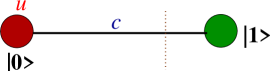
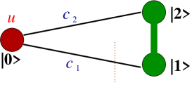
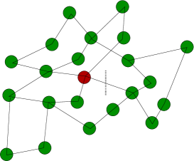
Figure 1: Two-site, three-site, and $1{+}N$ site models for transport. A particle is initially positioned at the “dot” site $|0\rangle$, The dot has a potential energy $u$ that can be controlled externally. As $u$ is varied, say from $-\infty$ to $+\infty$, currents are induced in the bonds of the network. Our objective is to calculate the current that flows from the dot to the network via a tagged bond. The vertical dotted line indicates a section through which the current of interest is flowing.

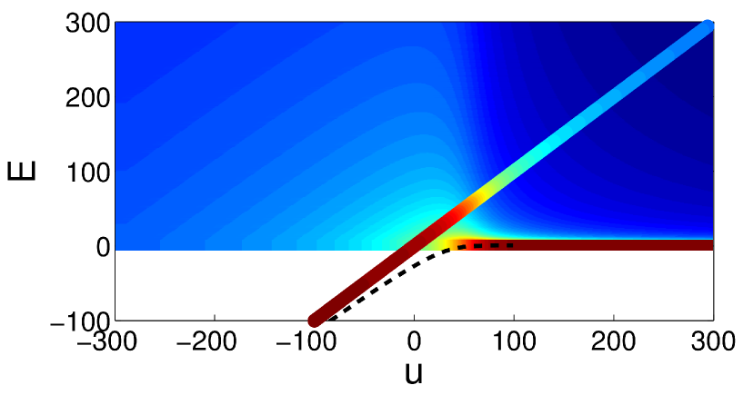
Figure 2: Upper panel: an initially loaded “dot” level is crossing a band that contains $N=500$ network levels. The occupation probabilities of the dot ($p$) and of the levels ($q_{n}$) are imaged as a function of time. The vertical axis is the energy, and the horizontal axis is $u(t)$. In this specific example the sweep process is adiabatically slow: As $u$ is increased the dot level gets emptied (color changing from red to blue), while at the end of the process only the ground level of the network is occupied (color changing from blue to red). We assume star geometry with level spacing $\Delta{=}1$, and identical couplings ${c_{n}{=}3}$. The dashed line illustrates the energy of the lowest adiabatic level. Lower panel: plot of $q_{n}$ vs $n$ in several cases. Green line with markers - the adiabatic scenario of the upper panel at $u=60$. Cyan solid line - after decay from a standing level ($\dot{u}{=}0$). Red dashed line - after decay from a moving level ($\dot{u}{=}5000$).

In this work we would like to analyze the following prototype problem. Consider a network as illustrated in Fig. 1. It consists of $N$ interconnected sites, with on-site energies $\mathcal{E}_{i}$, and couplings $C_{ij}$. Additionally there is a site ($i=0$) that we call “dot”, where the potential energy $\mathcal{E}_{0}=u(t)$ is varied according to some time-dependent protocol. For illustration purpose we assume that the on-site potential is swept monotonically from $u=-\infty$ to $u=\infty$. The Hamiltonian is

$$\mathcal{H}\ \ =\ \ \sum_{i=0}^{N}|i\rangle\mathcal{E}_{i}\langle i|\ +\ \sum_{i\neq j}|i\rangle C_{ij}\langle j|$$ (1)

$$\ \ \ \ \ \mathcal{E}_{0}{=}u(t),\ \ C_{i0}{=}C_{i}$$ (2)

Our interest is in the induced current $I(t)$ that flows through a tagged bond ${0\leadsto a}$ that connects the dot (${i=0}$) with some other network site (${i=a}$). This bond is reflected in the Hamiltonian by the presence of a coupling constant $C_{a0}=C_{a}$.

In order to have a well-posed problem we assume that there is no magnetic field: accordingly all the couplings can be gauged as real numbers; and there are no persistent currents in the network. In the adiabatic limit [6, 7, 8, 9, 10, 19, 20, 21, 22, 23] the current $I(t)$ is proportional at any moment to $\dot{u}$, and can be calculated as follows:

$$I=G\dot{u},\hskip 42.67912ptG=2\mbox{Im}\left[\Big{\langle}\frac{\partial}{\partial\phi}\Psi\Big{|}\frac{\partial}{\partial u}\Psi\Big{\rangle}\right]_{\phi=0}$$ (3)

Here $\phi$ is a test flux through the bond of interest, namely $C_{a}\mapsto C_{a}\mbox{e}^{i\phi}$, and $\Psi$ is the wave-function of the adiabatic eigenstate. The coefficient $G$ is known as the Geometric Conductance, or as the Berry-Kubo curvature. In [23] the interested reader can find how this formula is used in order to determine the current in the two-site and three-site models that are illustrated in Fig. 1.

The adiabatic transport formula Eq. (3) is not transparent: it requires some effort to get a heuristic understanding of its outcome. Furthermore it does not apply to non-adiabatic circumstances. We therefore look for a different way of calculation. Evidently for a two-site model, as illustrated in Fig. 1, we can simply use the continuity equation:

$$I=\frac{\partial}{\partial t}\left[q_{1}\right],\hskip 42.67912ptq_{1}=|\langle 1|\Psi(t)\rangle|^{2}$$ (4)

where $q_{1}$ is the occupation probability of the $i=1$ site. Clearly, this formula holds irrespective of whether the sweep process is adiabatic or not. Hence the problem of calculating currents trivially reduces to the calculation of a time-dependent occupation probability.

Considering a general network, our main observation is that for a multiple-path geometry the continuity equation can be generalized as follows:

$$I=\frac{\partial}{\partial t}\left[\sum_{n}\lambda_{n}q_{n}\right],\hskip 42.67912ptq_{n}=|\langle\epsilon_{n}|\Psi(t)\rangle|^{2}$$ (5)

Here the $q_{n}$ are the occupation probabilities of the network levels $|\epsilon_{n}\rangle$, and the pre-factors $\lambda_{n}$ are determined by the coupling constants. We refer to $\lambda_{n}$ as the splitting ratio: it describes the relative contribution of the ${0\leadsto n}$ flow to the current in the tagged bond. Hence, again, the calculation of the current reduces to that of calculating time-dependent probabilities, as in the stochastic formulation. But we shall see that the splitting ratios, unlike the branching ratios of the stochastic theory, are not bounded within ${[0,1]}$. For a non-interacting many-body occupation, results can be obtained by simple summation, with $q_{n}(t)$ that represent the actual occupations of the levels.

As already stated, for demonstration purpose, we are going to analyze a sweep process, in which the on-site potential is varied monotonically from $u=-\infty$ to $u=\infty$. We are going to distinguish between two sweep scenarios:

• Injection - the dot is initially filled with a particle that later is transferred to the network;

• Induction - one of the levels of the network is initially filled, and later a current is induced via the crossing dot.

The occupation dynamics in the first (Injection) scenario is illustrated in Fig. 2, which will be further discussed later. In later sections we consider also the second (Induction) scenario considering “star geometry” and “ring geometry”.

2 Star geometry, adiabatic limit

Let us consider the special geometry of a network that consists of sites $\mathcal{E}_{n}=\epsilon_{n}$, and connections $C_{n0}=c_{n}$, while all the other couplings are zero, as illustrated in the inset of Fig. 2. An adiabatic eigenstate $|\Psi\rangle$ is represented by a column vector ${\psi_{n}=\langle n|\Psi\rangle}$ that satisfies the following set of equations:

$$u\psi_{0}+\sum_{n=1}^{N}c_{n}^{*}\psi_{n} = E\psi_{0}$$ (6)

$$c_{n}\psi_{0}+\epsilon_{n}\psi_{n} = E\psi_{n},\ \ \ \ \ \ n=1,2,...,N$$ (7)

It follows from Eq. (7) that it can be written as:

$$|\Psi\rangle\ \ =\ \ \sqrt{p}\,|0\rangle\ +\ \sqrt{p}\sum_{n=1}^{N}\frac{c_{n}}{E-\epsilon_{n}}\,|n\rangle$$ (8)

where $\sqrt{p}$ is a normalization constant. We define

$$g(E;c_{1},...c_{N})\ \ =\ \ \sum\frac{|c_{n}|^{2}}{E-\epsilon_{n}}$$ (9)

Substitution of the $\psi_{n}$ of Eq. (8) into Eq. (6) leads to the secular equation ${g(E)=E-u}$ for the adiabatic eigen-energies. We focus our attention on a particular root $E(u)$. As $u$ is swept from $-\infty$ to $+\infty$, the energy $E(u)$ increases monotonically from $\epsilon_{n_{0}}$ to $\epsilon_{n_{0}+1}$, where $n_{0}$ is the starting level. From Eq. (8) it follows that $p$ is the probability to find the particle in the dot. It can be written as

$$p(u)\ \ =\ \ |\psi_{0}|^{2}\ \ =\ \ \Big{[}1-g^{\prime}(E(u))\Big{]}^{-1}$$ (10)

For the following derivation note that $1/p$ is a quadratic form in $c_{n}$, and that the occupation probabilities of the network levels ${n=1,2,3...}$ are

$$q_{n}(u)\ \ =\ \ |\psi_{n}|^{2}\ \ =\ \ \left|\frac{c_{n}}{E(u)-\epsilon_{n}}\right|^{2}\ p(u)$$ (11)

Using Eq. (3) we get after differentiation by parts that the current through $c_{n}$ is

$$G\ = \ \frac{|c_{n}|^{2}}{(E-\epsilon_{n})^{2}}\left(\frac{\partial p}{\partial u}\right)-2p\frac{|c_{n}|^{2}}{(E-\epsilon_{n})^{3}}\left(\frac{\partial E}{\partial u}\right)$$

$$= \ \frac{\partial}{\partial u}\left[\left(\frac{1}{2}\frac{\partial(1/p)}{\partial c_{n}}c_{n}\right)\ p\right]\ \ =\ \ \frac{\partial}{\partial u}\left[q_{n}\right]$$ (12)

We further discuss and generalize this trivial result below.

3 Multiple path geometry, adiabatic limit

Let us find what is the expression for $G$ in the case of a general network. It is natural to switch from the $\mathcal{E}_{i}$ basis to an $\epsilon_{n}$ basis that diagonalize the network Hamiltonian in the absence of the dot. Consequently getting a star geometry with

$$c_{n}\ \ =\ \ \sum_{i}\langle\epsilon_{n}|i\rangle C_{i}$$ (13)

An example for this procedure is presented in Section 5 with regard to the dot-wire ring geometry of Fig. 3. Our interest is in the current through a tagged bond $C_{a}$. We define the “splitting ratio” of the current that flows in the $n$th levels as

$$\lambda_{n}[\text{splitting}]\ =\ \frac{\langle\epsilon_{n}|a\rangle C_{a}}{c_{n}}\ =\ \frac{\langle\epsilon_{n}|a\rangle C_{a}}{\sum_{i=1}^{N}\langle\epsilon_{n}|i\rangle C_{i}}$$ (14)

A straightforward generalization of the derivation that leads to Eq. (12) implies that the current through $C_{a}$ is given by Eq. (5).

At this stage Eq. (5) is regarded as the outcome of adiabatic transport theory, while in the next section we shall provide its general derivation, and observe that it is a valid result also in non-adiabatic circumstances.

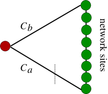
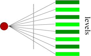
Figure 3: The dot-wire ring geometry (left). If the Hamiltonian is written in the $n$ basis the problem reduces to star geometry. The couplings of the levels to the dot are ${c_{n}\propto(C_{a}\pm C_{b})}$ for even or odd levels respectively. Hence it is like having two continua rather than a single continuum.

4 Transport calculation - the splitting ratio approach

Needless to say that we do not really need Eq. (3) in order to get the expression for $G$ in the case of a star graph. We could simply deduce Eq. (12) from conservation of probability, i.e. from the continuity equation $I=\dot{q}_{n}$. This is no longer the case if we have a multiple path geometry: probability conservation alone cannot tell us how the current is split between the different paths. Inspecting Eq. (5) it looks like a generalization of the continuity equation as discussed in the Introduction. Its physical simplicity suggests that it can be derived without assuming adiabaticity. We now show that this is indeed the case.

The stating point is the assumption that we have in hand the solution of the time-dependent Schrodinger equation, which can be written either in the $i$ or in the $\epsilon_{n}$ representations:

$$|\Psi(t)\rangle\ \ = \ \ \Psi_{0}(t)\,|0\rangle+\sum_{i=1}^{N}\Psi_{i}(t)\,|i\rangle$$ (15)

$$= \ \ \psi_{0}(t)\,|0\rangle+\sum_{n=1}^{N}\psi_{n}(t)\,|\epsilon_{n}\rangle$$ (16)

We recall our definitions of occupation probabilities:

$$p(t)\ \ = \ \ \langle 0|\Psi(t)\rangle\ \ =\ \ \ |\Psi_{0}(t)|^{2}\ \ =\ \ \mbox{dot occupation}$$ (17)

$$q_{n}(t)\ \ = \ \ \langle\epsilon_{n}|\Psi(t)\rangle\ \ =\ \ |\Psi_{n}(t)|^{2}\ \ =\ \ \mbox{level occupations}$$ (18)

and obviously the total occupation probability is unity:

$$p(t)\ +\ \sum_{n}q_{n}(t)\ \ =\ \ 1$$ (19)

In the $\epsilon_{n}$ basis the Hamiltonian becomes the same as in “Star geometry”. The current operator for the ${0\leadsto n}$ bond is

$$\mathcal{I}_{0\leadsto n}\ \ =\ \ -ic_{n}\,\Big{[}|n\rangle\langle 0|-|0\rangle\langle n|\Big{]}$$ (20)

Accordingly we can write the continuity equation

$$\dot{q}_{n}\ \ =\ \ \langle\Psi|\mathcal{I}_{0\leadsto n}|\Psi\rangle\ \ =\ \ c_{n}\,\mbox{Im}\left[\psi_{n}^{*}\psi_{0}\right]$$ (21)

But our interest is in the current that flows in real space through the tagged bond

$$I\ \ =\ \ \langle\Psi|\mathcal{I}_{0\leadsto a}|\Psi\rangle\ \ =\ \ C_{a}\ \mbox{Im}\left[\Psi_{a}(t)^{*}\Psi_{0}(t)\right]$$ (22)

The amplitudes $\Psi_{i}$ are related to the amplitudes $\psi_{n}$. In particular

$$\Psi_{a}(t)=\sum_{n}\langle a|\epsilon_{n}\rangle\ \psi_{n}(t),\ \ \ \ \ \ \ \ \ \Psi_{0}(t)=\psi_{0}(t)$$ (23)

Substitution of Eq. (23) into Eq. (22) gives

$$I\ \ =\ \ C_{a}\ \mbox{Im}\left[\sum_{n}\langle\epsilon_{n}|a\rangle\ \psi_{n}(t)^{*}\ \psi_{0}(t)\right]$$ (24)

Using the identification of $\dot{q}_{n}$ from Eq. (21) we get the desired result Eq. (5) with Eq. (14). This very simple, and yet very general result, has far reaching consequences as described below.

5 The dot-wire ring geometry

In order to demonstrate the application of the splitting ratio approach we shall consider the simplest non-trivial example, regarding the dot-wire ring geometry of Fig. 3. The ring consists of a “dot” whose potential $u(t)$ can be varied in time, and a “wire” that consists of ${i=1,...,N}$ sites with ${\mathcal{E}_{i}=0}$ and near-neighbor couplings $C_{ij}=C_{0}$. Optionally an appropriate procedure allows to take the limit $N\rightarrow\infty$ keeping the length of the wire ($L\equiv(1{+}N)a$) and the mass of the particle (${\mathsf{m}\propto 1/(C_{0}a^{2})}$) fixed. But the mathematics is more transparent with a tight binding model.

The energy levels of the wire are $\epsilon_{n}=-2C_{0}\cos(k_{n})$, where the wavenumbers are ${k_{n}=(\pi/L)n}$, with $L=N{+}1$. The respective couplings to the dot are

$$c_{n}\ \ =\ \ \left[\left(\frac{2}{L}\right)^{1/2}\sin(k_{n})\right]\ (C_{a}\pm C_{b})$$ (25)

where the $\pm$ reflects the parity of the level. It follows that the splitting ratios are

$$\lambda_{n}\ \ =\ \ \lambda_{\pm}\ \ =\ \ \frac{C_{a}}{C_{a}\pm C_{b}}\ \ \ \ \ \ \ \ \ \mbox{for level with even/odd parity}$$ (26)

In a later section we consider $N\gg 1$ wire, and focus on levels with wavenumber ${k_{n}\sim k}$ and energy ${\epsilon_{n}\sim E=-2C_{0}\cos(k)}$, that are located away from the band edges. In order to allow analytical treatment we assume that the density of states in the energy window of interest can be approximated as constant. Accordingly one can regard the level spacing $\Delta$ as a free parameter. In the same spirit it is convenient to absorb the constant pre-factor in Eq. (25) into the definition of $C_{a}$ and $C_{b}$, such that $c_{n}=(C_{a}\pm C_{b})/\sqrt{2}$.

6 The integrated current

From Eq. (5) it follows that the integrated current after a sweep process can be calculated as follows:

$$Q_{0\,\leadsto\,a}\ \ \equiv\ \ \int I(t^{\prime})\,dt^{\prime}\ \ =\ \ \sum_{n}\Big{[}q_{n}(\text{final})-q_{n}(\text{initial})\Big{]}\ \lambda_{n}$$ (27)

In particular for an Injection process

$$Q_{0\,\leadsto\,a}[\mbox{injection}]\ \ =\ \ \sum_{n}q_{n}(\text{final})\ \lambda_{n}$$ (28)

For an adiabatic injection scenario, in which the particle ends up at the lower network level we get

$$Q_{0\,\leadsto\,a}[\mbox{adiabatic injection}]\ \ =\ \ \lambda_{\mbox{ground level}}$$ (29)

while in the non-adibatic case the sum can be regarded as a weighted average of the $\lambda_{n}$. Let us consider for example the dot-wire ring system. For an adiabatic injection scenario we get

$$Q_{0\,\leadsto\,a}[\mbox{adiabatic injection}]\ \ =\ \ \lambda_{-}\ \ =\ \ \frac{C_{a}}{C_{a}{-}C_{b}}$$ (30)

Unlike the case of a stochastic transition this value is not bounded within ${[0,1]}$. rather it may have any value, depending on the relative sign of the amplitudes $C_{a}$ and $C_{b}$. But if the process is not adiabatic, the probability is distributed over both the odd and the even levels with probabilities that are proportional to ${|C_{a}\pm C_{b}|^{2}}$ respectively. Then we get from the weighted average a stochastic-like result, namely

$$Q_{0\,\leadsto\,a}[\mbox{fast injection}]\ \ =\ \ \text{average}(\lambda_{n})\ \ =\ \ \frac{|C_{a}|^{2}}{|C_{a}|^{2}+|C_{b}|^{2}}$$ (31)

For an adiabatic induction scenario, the particle is prepared (say) in an even wire-level, and is adiabatically transferred, due to the sweep, into the adjacent odd wire-level. Then we get

$$Q_{0\,\leadsto\,a}[\mbox{adiabatic induction}]\ \ =\ \ \lambda_{-}-\lambda_{+}\ \ =\ \ \frac{2C_{a}C_{b}}{|C_{a}|^{2}-|C_{b}|^{2}}$$ (32)

It looks as if the result does not depend on $C_{0}$. However this is misleading. In the next section we shall give a detailed account with regard to the time dependence of $I$, and we shall see that the induction process is significantly different depending on whether $C_{0}$ is small or large.

7 The parametric variation of the current

The results for the integrated current give the impression that the size of the coupling $c_{n}$ compared with the levels spacing $\Delta$ is of no importance. But this is a wrong impression. Once we get deeper into the analysis it becomes clear that the familiar two level approximation for the adiabatic current $I$, requires the coupling $c_{n}$ to be very small compared with the level spacing $\Delta$. Our interest below is focused in the case of having a quasi-continuum, meaning that the $c_{n}$ are larger than $\Delta$, hence many levels are mixed during the sweep process.

Before discussing the quasi-continuum case it is useful to note that the 3 site ($N=2$) ring system has been solved exactly in [23]. It has been found that if the $c_{n}$ are not smaller compared with $\Delta$, the dot-induced mixing of the levels modifies the functional form of $G(u)$ in a non-trivial way.

We now turn to discuss what happens with $N\gg 1$ dot-wire system. In Fig. 5 we show how the occupations of the levels change as $u$ is swept during an adiabatic induction process. Initially only level $n_{0}=250$ is occupied, while at the end of the sweep the probability is fully transferred to $n=251$. The figure assumes ${c_{n}\gg\Delta}$, and therefore during the process many other levels are occupied. This is what we call quasi-continuum case. In the other extreme of having ${c_{n}\ll\Delta}$, only 3 levels participate in the scenario: the dot level and the network levels ${n=250,251}$. In the latter case there are two distinct crossings, each can be described as a two-level crossing, with current dependence that is shown in the upper panel of Fig. 5. In contrast to that, in the quasi continuum case, individual crossings with the network levels cannot be resolved. Rather we see in the lower panel of Fig. 5 that there is a single wide collective peak in the current that extends over an energy range that contains many network levels. It is the purpose of the next section to get an analytical understanding of this multi-level mixing, and to obtain an explicit result for the current dependence.

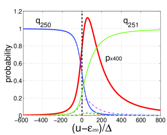
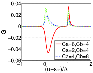
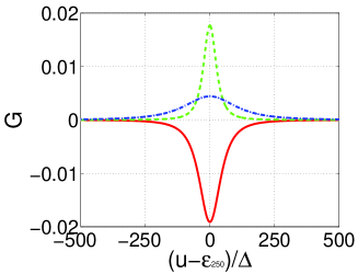
Figure 4: We consider an adiabatic sweep of an empty dot level through a wire that is occupied by a single particle. The particle is initially placed at $n_{0}=250$ (an arbitrary level). The variation of the occupation probabilities is plotted as a function of $u$. The level spacing is ${\Delta=1}$, and the couplings are $C_{a}=6$ and $C_{b}=4$. Accordingly the couplings to the even and to the odd levels are $c_{\pm}=(C_{a}\pm C_{b})/\sqrt{2}$. The red thick line is the dot occupation $p$, with vertical scale that is magnified ${\times 400}$. The other solid lines are $q_{250}$, and $q_{251}$. The dashed lines from up to down are $q_{249}$ and $q_{253}$ and $q_{247}$ and $q_{252}$.

Figure 5: Flow of the current from the dot to the wire through the $C_{a}$ bond, for the same scenario as in Fig. 5. The parameters are indicted in the legend. The raw calculation is done using Eq. (40) with Eq. (10). In the upper panel ${\Delta=200}$, hence a two-level approximation for each crossing is satisfactory. In the lower panel ${\Delta=1}$, hence the explicit result Eq. (43) can be optionally used in order to describe the multi-level crossing.

8 Adiabatic mixing in quasi continuum

We turn to the detailed analysis of adiabatic mixing in the dot-wire system. The first step is to get an expression for $g(E)$ of Eq. (9). With $c_{n}=c_{\pm}$ the sum over the levels splits into two partial sums, over the odd and over the even levels. Consequently after summation we get two terms:

$$g(E)=\left(\frac{\pi}{2\Delta}\right)\left[c_{-}^{2}\cot\left(\pi\frac{E}{2\Delta}\right)-c_{+}^{2}\tan\left(\pi\frac{E}{2\Delta}\right)\right]$$ (33)

The secular equation ${g(E)=E-u}$ becomes a quadratic equation for $\cot()$, and can be solved explicitly:

$$\cot\left(\pi\frac{E}{2\Delta}\right)=\frac{\Delta}{\pi c_{-}^{2}}\left[(E{-}u)\pm\sqrt{(E{-}u)^{2}+\left(\frac{\pi c_{+}c_{-}}{\Delta}\right)^{2}}\right]$$ (34)

where the $\pm$ refers to the parity that is alternating for subsequent levels. Then it is straightforward to get an explicit expression for the dot occupation probability $p(u)$ via Eq. (10), and for the level occupations $q_{n}(u)$ via Eq. (11). The expressions are quite lengthy but can be simplified in the regime of interest as described below.

Of interest is the case of a quasi-continuum, meaning that the couplings $c_{n}$ are larger compared with $\Delta$, hence a two level approximation is out of the question, while a Wigner-type approximation is most appropriate. For this purpose we find it useful to define parameters that describe the effective coupling of the dot to the quasi-continuum, and its asymmetry:

$$C_{\text{eff}} \equiv \ \ \frac{\pi}{2}\frac{c_{+}c_{-}}{\Delta}$$ (35)

$$\Gamma \equiv \pi\frac{c_{+}^{2}+c_{-}^{2}}{\Delta}$$ (36)

$$\sin(\theta) \equiv \frac{c_{+}^{2}-c_{-}^{2}}{c_{+}^{2}+c_{-}^{2}}$$ (37)

Here and below we assume without loss of generality that the particle starts in an even-parity level. Using these notations we get after some algebra an approximation that should be valid in the quasi-continuum case:

$$p(u)\ \ \approx\ \ \Delta\cdot\mathrm{L}\left[u-E;\ \Gamma,\theta\right]$$ (38)

The distorted Lorentzian $\mathrm{L}\left[x;\Gamma;\theta\right]$ is

$$\frac{1}{\pi}\left[1+\frac{\sin\theta\ x}{\sqrt{x^{2}+\cos^{2}\theta\ (\Gamma/2)^{2}}}\right]^{-1}\frac{\cos^{2}\theta\ (\Gamma/2)}{x^{2}+\cos^{2}\theta\ (\Gamma/2)^{2}}$$ (39)

In the expression above $E$ is the energy in which the particle has been prepared. In the regime of interest, where the levels are treated as quasi-continuum, this energy can be regarded as a constant. Some further straightforward algebra leads to

$$G(u) = C_{a}\frac{\partial}{\partial u}\left[p\sum_{n}\frac{c_{n}^{*}\langle n|a\rangle}{(E-\epsilon_{n})^{2}}\right]$$ (40)

$$= C_{a}\frac{\partial}{\partial u}\left[\frac{\frac{c_{-}}{\sin^{2}\left(\pi\frac{E}{2\Delta}\right)}+\frac{c_{+}}{\cos^{2}\left(\pi\frac{E}{2\Delta}\right)}}{\left(\frac{2\Delta}{\pi}\right)^{2}+\frac{c_{-}^{2}}{\sin^{2}\left(\pi\frac{E}{2\Delta}\right)}+\frac{c_{+}^{2}}{\cos^{2}\left(\pi\frac{E}{2\Delta}\right)}}\right]$$ (41)

$$\approx \frac{\partial}{\partial u}C_{a}\left[\frac{c_{+}+c_{-}\cot^{2}\left(\pi\frac{E}{2\Delta}\right)}{c_{+}^{2}+c_{-}^{2}\cot^{2}\left(\pi\frac{E}{2\Delta}\right)}\right]$$ (42)

$$= (\lambda_{-}-\lambda_{+})\frac{2C_{\text{eff}}^{2}}{\left(4C_{\text{eff}}^{2}+(u-E)^{2}\right)^{3/2}}$$ (43)

Disregarding the splitting-ratio factor, this expression has surprisingly the same functional form as that of crossing a single level ($N=1$), see e.g. [23], but with an effective coupling constant $C_{\text{eff}}$ that reflects the density of states.

The functions $p(u)$ and $G(u)$ are plotted in Fig. 5 and in Fig. 5. In the latter we contrast with the ${c_{n}\ll\Delta}$ case, for which the dynamics can be regarded as a sequence of two $N=1$ crossings.

9 Adiabatic and non-adiabatic regimes

The results for the integrated current give another wrong impression: it looks as if we are dealing with two regimes: either the process is adiabatic or non-adiabatic. A more careful inspection reveals that depending on $\dot{u}$ we have 3 regimes: Adiabatic, Slow and Fast. For star geometry with comb-like quasi continuum of levels, the Slow regime is defined by the condition

$$c^{2}\ <\ \dot{u}\ <\ \Gamma^{2},\ \ \ \ \ \ \Gamma\equiv 2\pi\frac{c^{2}}{\Delta}$$ (44)

For simplicity we assume here comb-like quasi continuum with identical couplings ${c_{n}=c}$. The left inequality in Eq. (44) means that the adiabatic condition is violated, while the right inequality implies that a first-order perturbative approximation is violated as well. The identification of this intermediate Slow regime parallels the notion of Wigner or FGR or Kubo regime in past studies of time-dependent dynamics [19].

Some illustrations for energy spreading are presented in Fig. 2. If ${c<\Delta}$ the transport of probability from the dot to the network levels would be described using a two-level approximation. But the illustration in the upper panel assumes ${c>\Delta}$, hence many levels are mixed within a parametric range $\Gamma$. The time during which this mixing takes place is $\Gamma/\dot{u}$. In the opposite limit of Fast sweep, which we further discuss below, the decay time of the probability to the quasi-continuum is $1/\Gamma$.

10 Non adiabatic spreading

The calculation of $I$ in the non-adiabatic regime requires knowledge of $q_{n}(t)$. For star geometry this calculation is a variant of the Wigner decay problem, and hence can be solved analytically: instead of a fixed level that decays into a quasi-continuum we have a moving level. The usual textbook procedure is followed [31] leading to the following set of equations

$$\partial_{t}\Psi_{0} = \Big{[}-iu(t)-(\Gamma/2)\Big{]}\Psi_{0}$$ (45)

$$\partial_{t}\Psi_{n} = -i\epsilon_{n}\Psi_{n}-ic_{n}\Psi_{0}$$ (46)

With ${u(t)=\dot{u}t}$ one obtains the solution

$$q_{n}(t)\ =\ \left|c_{n}\int_{0}^{t}d\tau\ \exp\left(i\epsilon_{n}\tau-i\frac{\dot{u}}{2}\tau^{2}-\frac{\Gamma}{2}\tau\right)\right|^{2}$$ (47)

By inspection one observes that going from the Slow to the Fast regime, the spreading line shape changes from Lorentzian-type to Fresnel-type, as illustrated in the lower panel of Fig. 2.

11 Summary

Molecular motors and pumps are of great interest in various fields of Physics and Biology. Conceptually the major theme concerns the possibility to induce a circulating motion, or a circulating current, by some driving protocol. We use the term stirring rather than pumping in order to emphasize that closed geometry is concerned (no reservoirs). Considering (e.g.) the unidirectional rotation of a molecular rotor [27], it is possibly allowed to be satisfied with a stochastic picture [26] that relates the currents, via a “decomposition formula”, to rates of change of occupation probabilities. Once we turn (e.g.) to the analysis of pericyclic reactions [30] this is no longer possible. In the latter case the method of calculating electronic quantum fluxes had assumed that they can be deduced from the continuity equation. Such procedure is obviously not applicable for (say) a ring-shaped molecule: due to the multiple path geometry there is no obvious relation between currents and time variation of probabilities.

Nevertheless, we have found using elementary considerations, that it is possible to replace the traditional adiabatic transport formula Eq. (3) by a simple expression Eq. (5), that holds both in adiabatic and non-adiabatic circumstances. It can be regarded as a generalized multi-path generalization of the continuity equation. Hence the problem of calculating currents is reduced to that of calculating time-dependent probabilities $q_{n}(t)$ as in the above mentioned stochastic formulation.

Our result Eq. (5) is quite general. We have demonstrated its use in the very simple case of “ring geometry”, but it can be applied to any network configuration, and for any $u(t)$ time dependence. In particular one can use it in order to analyze a multi-cycle stirring process. Furthermore, the application of Eq. (5) to a many-body system of non-interacting particles follows trivially, with $q_{n}(t)$ that represent the actual occupations of the levels.

It is important to realize that the “splitting ratio” Eq. (14) unlike the stochastic “partitioning ratio” is not bounded within $[0,1]$. This observation has implications on the calculation of “counting statistics” and “shot noise” [32, 33, 34].

We have emphasized aspects that go beyond the familiar two-level approximation phenomenology, related to the scrambling of the network levels during the sweep process. The dot-induced mixing is reflected in the time dependence of the currents, but not in $Q$.

Acknowledgments.– This research has been supported by the Israel Science Foundation (grant No.29/11).

References

References

- [1] J.E. Avron, D. Osadchy, R. Seiler, Physics Today 56, 38 (2003).
- [2] M. Mottonen, J.P. Pekola, J.J. Vartiainen, V. Brosco, F.W.J. Hekking, Phys. Rev. B 73, 214523 (2006͒).
- [3] J.I. Cirac, P. Zoller, H.J. Kimble, H. Mabuchi, Phys. Rev. Lett. 78, 3221 (1997)
- [4] H.J. Kimble, Nature 453, 1023 (2008)
- [5] S. Engel et. al, Nature 446, 782 (2007)
- [6] D.J. Thouless, Phys. Rev. B 27, 6083 (1983).
- [7] Q. Niu and D. J. Thouless, J. Phys. A 17, 2453 (1984).
- [8] M.V. Berry, Proc. R. Soc. Lond. A 392, 45 (1984).
- [9] J.E. Avron, A. Raveh and B. Zur, Rev. Mod. Phys. 60, 873 (1988).
- [10] M.V. Berry and J.M. Robbins, Proc. R. Soc. Lond. A 442, 659 (1993).
- [11] M. Buttiker, H. Thomas, A Pretre, Z. Phys. B Cond. Mat. 94, 133 (1994).
- [12] P. W. Brouwer, Phys. Rev. B 58, R10135 (1998)
- [13] B.L. Altshuler, L.I. Glazman, Science 283, 1864 (1999).
- [14] M. Switkes, C.M. Marcus, K. Campman, A.C.Gossard Science 283, 1905 (1999).
- [15] J.A. Avron, A. Elgart, G.M. Graf, L. Sadun, Phys. Rev. B 62, R10618 (2000).
- [16] D. Cohen, Phys. Rev. B 68, 201303(R) (2003).
- [17] L.E.F. Foa Torres, Phys. Rev. Lett. 91, 116801 (2003); Phys. Rev. B 72, 245339 (2005).
- [18] O. Entin-Wohlman, A. Aharony, Y. Levinson, Phys. Rev. B 65, 195411 (2002).
- [19] D. Cohen, Phys. Rev. B 68, 155303 (2003).
- [20] D. Cohen, T. Kottos, H. Schanz, Phys. Rev. E 71, 035202(R) (2005).
- [21] G. Rosenberg and D. Cohen, J. Phys. A 39, 2287 (2006).
- [22] I. Sela, D. Cohen, J. Phys. A 39, 3575 (2006); Phys. Rev. B 77, 245440 (2008).
- [23] D. Davidovich, D. Cohen, J. Phys. A 46, 085302 (2013).
- [24] C. Zener, Proc. R. Soc. Lond. A 317, 61 (1932).
- [25] N.V. Vitanov, B.M. Garraway, Phys. Rev. A 53 4288 (1996).
- [26] S. Rahav, J. Horowitz, C. Jarzynski, Phys. Rev. Lett., 101, 140602 (2008).
- [27] D. A. Leigh, J.K.Y. Wong, F. Dehez, F. Zerbetto, Nature (London) 424, 174 (2003)
- [28] J.M.R. Parrondo, Phys. Rev. E 57, 7297 (1998)
- [29] R.D. Astumian, Phys. Rev. Lett. 91, 118102 (2003).
- [30] D. Andrae, I. Barth, T. Bredtmann, H.-C. Hege, J. Manz, F. Marquardt, and B. Paulus, J. Phys. Chem. B, 115, pp 5476 (2011).
- [31] See for example section 43 of arXiv:quant-ph/0605180v4
- [32] L.S. Levitov, G.B. Lesovik, JETP Lett. 58, 230 (1993͒).
- [33] Y.V. Nazarov, M. Kindermann, Eur. Phys. J. B 35, 413 (2003͒).
- [34] M. Chuchem, D. Cohen, J. Phys. A 41, 075302 (2008); Phys. Rev. A 77, 012109 (2008); Physica E 42, 555 (2010).