Abstract

Most neurons in peripheral sensory pathways initially respond vigorously when a preferred stimulus is presented, but adapt as stimulation continues. It is unclear how this phenomenon affects stimulus representation in the later stages of cortical sensory processing. Here, we show that a temporally sparse and reliable stimulus representation develops naturally in a network with adapting neurons. We find that cellular adaptation plays a critical role in the transient reduction of the trial-by-trial variability of cortical spiking, providing an explanation for a wide-spread and hitherto unexplained phenomenon by a simple mechanism. In insect olfaction, cellular adaptation is sufficient to explain the emergence of the temporally sparse and reliable stimulus representation in the mushroom body, independent of inhibitory mechanisms. Our results reveal a computational principle that relates neuronal firing rate adaptation to temporal sparse coding and variability suppression in nervous systems with a sequential processing architecture.

Introduction

The phenomenon of spike-frequency adaptation (SFA)[1] (also known as spike-rate adaptation) is a fundamental process in nervous systems, which attenuates the neuronal stimulus responses to a lower level following an initial high firing. This process can be mediated by different cell-intrinsic mechanisms that involve a spike-triggered self-inhibition, and which can operate in a wide range of time scales[3, 25]. These processes are probably related to the early evolution of the excitable membrane[38, 36] and are common to vertebrate and invertebrate neurons, both in the peripheral and central nervous system[49]. Nonetheless, the functional consequences of SFA in peripheral stages of sensory processing on the representation of stimuli in later network stages remain unclear. For instance, while olfactory stimuli generally display a slow kinetics, the early olfactory system shows temporally adaptive and precise onset responses[40, 19], that may translate into narrow integration windows for the principal neurons in the next processing stage, the piriform cortex pyramidal cells in rodents[35] and the mushroom body Kenyon cells in insects[34]. However, it remains unclear how sparse single-neuron responses can reliably encode information in face of the response variability[41] and the sensitivity of cortical networks to small perturbations[24].

Here, we show that the SFA mechanism introduces a dynamical non-linearity in the transfer function of neurons. Subsequently, the response onset becomes progressively sparser when transmitted across successive processing stages. Additionally, the self-regulating effect of SFA causes a stimulus-triggered reduction of firing variability by modulating the average inhibition in the balanced cortical network. In this manner the temporally sparse representation is accompanied by an increased response reliability. Using this theoretical framework on data obtained from the olfactory system of the honeybee, we show that the sequential effect of the SFA shapes the Kenyon cells’ temporal sparseness independent of inhibitory synaptic mechanisms.

Our results reveal a generic, biophysically plausible mechanism that can explain the emergence of a reliable and sparse stimulus representation, indicating the importance of cellular adaptation in sensory computation at the network level.

RESULTS

Temporal sparseness emerges in successive adapting populations

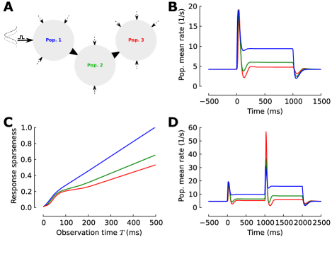
Figure 1: Neuronal adaptation in the multi-stage processing network. (A) Schematic illustration of a three-layered model of an adaptive pathway of sensory processing. The network consists of three consecutive adaptive populations. Each population receives sensory input from an afferent source (black arrows) and independent constant background excitation (dashed arrow). Input is modeled by a Gaussian density and a sensory stimulus presented to the first population is modeled by an increase in the mean input value. (B) Response profiles. The evoked state consists of a phasic-tonic response in all populations. The tonic response level is decremented across the consequtive populations. (C) Temporal sparseness $S_{r}^{i}$ is measured by the integral over the firing rate and normalized by the average spike count at $t=500\,$ms in the first population. Responses become progressively sparser as the stimulus propagates into the network. (D) Secondary response profiles. The additional jump increase in stimulus strength at $t=1000\,$ms during the evoked state of the first stimulus results in a secondary phasic response in all populations with an amplitude overshoot in the 2nd and 3rd population.

To examine how successive adapting populations can achieve temporal sparseness, first we mathematically analyzed a sequence of neuronal ensembles (Figure 1A), where each ensemble exhibits a generic model of mean firing rate adaptation by means of a slow negative self-feedback[3, 22, 29] (Materials and Methods). This sequence of neuronal ensembles should be viewed as caricature for distinct stages in the pathway of sensory processing. For instance in the mammalian olfactory system the sensory pathway involves several stages from the olfactory sensory neurons to the olfactory bulb, the piriform cortex, and then to higher cortical areas (Figure 1A).

The mean firing rate in the steady-state of a single adaptive population can be obtained by solving the rate consistency equation, $\bar{r}_{i}=f(\mu_{i}-\tau_{s}q_{s}\bar{r}_{i}|\sigma_{i}^{2})$, where $\bar{r}$ is the equilibrium mean firing rate of the population $i$, $\mu_{i}$ and $\sigma_{i}^{2}$ are mean and variance of the total input into the population, respectively, $f$ is the response function (input-output transfer function, or $fI$-curve) of the population mean activity, $q_{s}$ is the quantal conductance of the adaptation mechanism per unit of firing rate, and $\tau_{s}$ is the firing rate relaxation time constant[3, 22, 29]. It is known that any sufficiently slow modulation ($1/r_{max}<\tau_{s}$) linearizes the steady-state solution, $\bar{r}_{i}$, due to the self-inhibitory feedback being proportional to the firing rate[10].

Here, for simplicity, we studied the case where all populations in the network exhibit the same initial steady-state rate. This is achieved by adjustment of a constant background input to population $i$ (doted arrows, Figure 1A), resembling the stimulus irrelevant interactions in the network. All populations are coupled by the same strength $g$. First, we calculated the average firing rate dynamics of the populations’ responses following a step increase in the mean input to the first layer (black arrow, Figure 1A). By solving the dynamics of the mean firing rate and adaptation level concurrently, we obtained the mean-field approximation of the populations’ firing rates (Materials and Methods). The responses of each population consisted of a phasic and a tonic part, typical for adapting neurons. Here, we plotted the mean firing rate of three consecutive populations (Figure 1B). The phasic response to a step increase in the input is presented across stages. However, the tonic response becomes increasingly suppressed in the later stages (Figure 1B). This phenomenon is a general feature of successive adaptive neuronal populations. To understand why the tonic response part, after the adaptation was reinstalled, is increasingly suppressed in later stages we used the linearity of the adaptive transfer function and its stability conditions at the steady-state[10]. Thus, a change in the mean rate of population $i$ is the solution of $\Delta{\bar{r}}_{i}=f(g\Delta\bar{r}_{i-1}-\Delta{\bar{r}}_{i}\tau_{s}q_{s})$, and since the transfer function, $f$, is assumed to be increasing and the slope of $\bar{r}$ is less than unity, the solution can only existe for $\Delta{\bar{r}}_{i-1}>\Delta{\bar{r}}_{i}$ (Materials and Methods). The result in this sub-section (Figure 1B-C) was established with a current based leaky integrated-and-fire response function. However, the analysis presented here extends to the majority of neuronal transfer functions since the stability and linearity of the adapted steady-states are granted[10, 22]. This simple effect leads to a progressively sparser representation across successive stage of a generic feed-forward adaptive processing. We quantified the temporal sparseness by $S_{r}^{i}(T)=\int_{0}^{T}r_{i}(t)dt$, where $r_{i}(t)$ is the mean firing rate of population $i$ and $T$ is the observation time window. Normalization of this measure by the first population $S_{r}^{1}(T=500)$ indicates sparser responses in later stages of the adaptive network (Figure 1C).

Does the suppression of the adapted response level impair the information about the presence of the stimulus? To explore this, we studied a secondary increase in stimulus strengths of equal magnitude after 1 second when the network has relaxed to the evoked equilibrium (Figure 1D). The secondary stimulus jump induced a secondary phasic response of comparable magnitude in the first population (Figure 1D). However, in the later populations this jump evoked an icreased peak rate in the phasic response (Figure 1D). Notably, the coupling factor $g$ between the populations shapes this phenomena. Here, we adjusted $g$ to achieve an equal onset response magnitude across the populations for the first stimulus jump at $t=0$, and a slight increase in the population onset response in the first population is amplified in the later stages. This is due to the fact that the later stages accumulated less adaptation in their evoked steady-state (level of adaption is proportional to mean firing rate). Importantly, this result confirms that the sustained presence of the stimulus is indeed stored in the level of cellular adaptation[32], even though it is not reflected in the firing rate of the last population. Therefore, regardless of the absolute amplitude of responses, the relative relation between secondary and initial onset keeps increasing across layers. This type of a secondary overshoot is also experimentally known as sensory sensitization, where an additional increase in the stimulus strength significantly enhances the responsiveness of later stages after the network converged to an adapted steady-state[18].

Adaptation increases response reliability in the cortical network

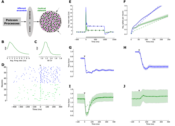
Figure 2: Reliability of a temporally sparse code in the balanced cortical network. (A) Schematic of a two-layer model of sub-cortical and early cortical sensory processing. The afferent ensemble (blue) consists of 4,000 independent neurons, and each neuron projects to 1% of the neurons in the cortical network (green). The cortical network is a balanced network in the asynchronous and irregular state with random connectivity. In both populations black circles represent excitatory neurons and magenta circles represent inhibitory cells. (B) The distribution of firing rates across neurons in the cortical network is fat-tailed and the average firing rate is approximately 3Hz. (C) The distribution of the coefficient of variation ($C_{v}$) across neurons in the balanced cortical network confirms irregular spiking. (D) Spike raster plot for a sample set of 30 afferent neurons (blue dots) and 30 excitatory cortical neurons (green dots). At $t=0$ (gray triangle) the stimulus presentation starts. (E) Population averaged firing for both network stages. The simulation (solid lines) follows the calculated ensemble average predicted by the adaptive density treatment (black circles). The firing rate in the simulated network is estimated with a 20ms bin size. (F) Number of spikes per neuron $S_{e}$ after stimulus onset ($t=0$) for the adaptive network (solid lines) and the weakly adaptive control network (dashed lines). Cortical excitatory neurons (green) produced less spikes than neurons in the earlier stage (afferent ensemble, blue). The shaded area indicates the standard deviation across neurons. (G,H) Fano factor dynamics of the afferent ensemble in the network with strongly adapting neurons (G, $\tau_{s}=110\,$ms) and in the weakly-adaptive (h, $\tau_{s}=30\,$ms) network, estimated across 200 trials in a 50ms window and a sliding of 10ms for the ensemble network with adaptation. The black circles indicate the theoretical value of the Fano factor computed by adaptive density treatment and shaded area is the standard deviation of the Fano factor across neurons in the network. (I) The Fano factor of strongly adaptive neurons in cortical balanced network reduced transiently during the initial phasic response part. The crosses show the adaptive cortical ensemble Fano factor for the case where the afferent ensemble neurons were modeled as a Poisson process with the same steady-state firing rate and without adaption. (J) The Fano factor in the weakly adaptive cortical network did not exhibit a reduction during stimulation.

The mean firing rate approach as above is insufficient to determine how reliable the observed response transients are across repeated stimulations. In the prevailing spiking network model of the cortex, the balance of excitation and inhibition is quickly reinstalled within milliseconds after the onset of an excitatory input[47] and self-generating recurrent fluctuations strongly dominate the dynamics of the interactions. It has thus been questioned whether a sparse response of only very few action potentials could reliably encode the presence of a stimulus[24].

To investigate the reliability of adaptive mapping from a dense stimulus to a sparse cortical spkie response across successive processing stages we employed an adaptive population density formalisms[29, 11] (Materials and Methods) along with numerical network simulations. We embeded a two-layered sensory network with an afferent ensemble projecting to a cortical network (Figure 2A). The afferent ensemble consisted of 4,000 adaptive neurons that included voltage dynamics, conductance-based synapses, and spike-induced adaptation[29]. It resembles the sub-cortical sensory processing and each neuron in the afferent ensemble projects to randomly 1% of the neurons in the cortical network. This is a large circuit of the balanced network (Figure 2A) with 10,000 excitatory and 2,500 inhibitory neurons with a typical random diluted connectivity of 1%. The spiking neuron model in the cortical network again includes voltage dynamics, conductance-based synapses, and spike-induced adaptation[29]. All neurons are alike and parameters are given in Table.3 in Muller et al.[29]. With appropriate adjustment of the synaptic weights, the cortical network operates in a globally balanced manner, producing irregular, asynchronous activity[47, 20, 48]. The distribution of firing rates for the network approximates a power-law density[37] with an average firing rate of $\approx 3.0\,$Hz (Figure 2B) and the coefficients of variation ($C_{v}$) for the inter-spike intervals is centered at a value slightly greater than unity (Figure 2C) indicating the globally balanced and irregular state of the network[48]. Noteworthy, the activity of neurons in both stages is fairly incoherent and spiking in each sub-network is independent. Therefore, one can apply an adiabatic elimination of the fast variables and formulate a population density description where a detailed neuron model reduces to a stochastic point process [29, 11] that provides an analytical approximation and understanding of the simulation results in this section (Materials and Methods).

The background input is modeled as a set of independent Poisson processes that drive both sub-networks (dashed arrows, Figure 2A). The stimulus dependent input is an increase in the intensity of the Poisson input into the afferent ensemble (solid arrow, Figure 2A). 
Before 
the 
stimulus became active at time $t=0$, a
 typical 
neuron 
showed 
an 
irregular 
spiking activity in both network stages (Figure 2B-D). However, 
when 
a 
sufficiently
 strong
 stimulus
 is 
applied, neurons in both stages exhibited a transient response before the population mean firing rate converges back to a new level of steady-state (Figure 2D,E). The population firing rate in the numerical simulations (solid line, Figure 2E) follow well the adaptive population density treatment (filled circles, Figure 2E).

To measure the effect of neuronal adaptation on the temporal sparseness, we again computed the number of spikes per neuron after the stimulus onset, $S_{e}(T)$. We compare our standard adaptive network with an adaptation time constant of $\tau_{s}=$ 110ms (solid lines, Figure 2F) with an only weakly-adaptive control network ($\tau_{s}=$30ms; dashed lines, Figure 2F). Note, that the adaptation time constant in the weakly adaptive network is about equal to the membrane time constant and therefore plays a minor role for the network dynamics. It showed that both sub-networks generated sharp phasic response, which in the case of the cortical network evoked a single sharply timed spike within the first $\approx 10-20\,$ms in a subset of neurons (Figure 2B,F). In the control case, the response is non-sparse and response spikes are distrubuted throughout the stimulus period (dashed lines, Figure 2F). Overall, strong adaptation reduces the total number of stimulus-induced action potentials per neuron and concentrates their occurrence within an initial brief phase following fast changes in the stimulus. Thus, in accordance with the results of the rate-based model in the previous section, one can conclude that the sequential stimulation of adaptive network stages can account for the emergence of a sparse stimulus representation in a cortical population.

To 
reveal the effect of adaptation on the response variability, we employed the time-resolved Fano factor[31], $F$, which measures the spike-count variance divided by the mean spike count across $200$ repeated stimulations. Spikes were counted in a 50ms time window and a sliding of 10ms[9]. As before, we compared our standard adaptive network (Figure 2G,I; $\tau_{s}$ = 110ms) with the control network (Figure 2H,J; $\tau_{s}$=30ms). Since the Fano factor is known to be strongly dependent on the firing rate, we adjusted the input to the latter such that the steady state firing rates in both networks were mean-matched[9]. The input Poisson spike trains ($F=1$) translated into slightly more regular spontaneous ($t<0$) activity in the afferent ensemble (Figure 2G), as neuronal membrane filtering and refractoriness reduced the output variability. After the stimulus onset ($t=0$), due to the increase in the mean input rate, the average firing rate increased, however the variance of the number of events per trial did not increase proportionally. Therefore, we observed a reduction in the Fano factor (Figure 2G). This phenomena is independent of the adaptation mechanism in the neuron model and a quantitatively similar reduction can be observed in the weakly adaptive afferent ensemble (Figure 2H). A comparison between our standard adaptive and the control case reveals that the adaptive network is generally more regular in the background and in the evoked state (Figure 2G,H). This is due to the previously known effect, where adaptation induces negative serial correlations in the inter-spike intervals[5, 11] and as a result reduces the Fano factor[11, 7].

In the next stage of processing, the distribution of $F$ across neurons during spontaneous activity is high due to the self-generated noise of the balanced circuits[47, 23]. This closely follows a wide spread experimental finding where $F>1$ in the spontaneous cortical activity[9] ( Figure 2G,H). Whenever a sufficiently
 strong
 stimulus 
was applied, the 
internally 
generated 
fluctuations
 in the adaptive balanced network were transiently suppressed,
 and as a result the Fano factor dropped sharply (Figure 2I). However, this reduction of the Fano factor is a temporary phenomenon and $F$ converges back to slightly above the baseline variability (Figure 2I). At the same time, the evoked steady-state firing returned back to the irregular and asynchronous state (Figure 2D). Indeed, this effect corresponds to a temporally mis-match in the balanced input conditions to the cortical neurons since the self-inhibitory and slower adaption effect prevents a rapid adjustment to the new input regime. This can be observed in the time course of variability suppression that closely reflects the time constant of adaptation (Figure 2I). The afferent ensemble structured the input to the cortical ensemble, determining the magnitude of the observed reduction effect, and under the control condition where a pure Poisson input is provided to the cortical balanced network, the reduction in $F$ is reduced but the time scale of recovery remains unaltered (crosses, Figure 2I). We 
contrast 
this adaptive 
behavior
 with the variability dynamics in the weakly adaptive balanced network (Figure 2J). In 
this 
case there 
is 
no 
reduction
 in
 $F$, because for a short adaptation time constant the convergence to the balanced state is very rapid[47]. The small increase in the input noise strength leads to an increase of the self-generated randomness of the balanced network[28, 23].

To further understand the effect of the recurrent connectivity on the variability, one can compare the evoked variability between the afferent ensemble and the cortical network. In the latter, fluctuation intrinsic to the cortical networks dynamically bring back the cortical circuits to the spontaneous level of high variability within the time scale of adaption relaxation (Figure 2I). This suggests the transient suppression of variability during a stimulus response as a cortical-wide effect[9] could be caused by slow adjustment of self-regulatory feedback.

Adaptive networks generate sparse and reliable responses in the insect olfactory system

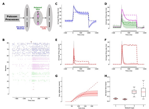
Figure 3: Neuronal adaptation generates temporal sparseness in a generic model of the insect olfactory network. (A) Schematic drawing of a simplified model of the insect olfactory network for a single pathway of odor coding. Olfactory receptor neurons (OSNs, first layer, n=1,480) project to the antennal lobe network (second layer) consisting of projection neurons (PNs, n=24) and local neurons (magenta, n=96), which make inhibitory connections with PNs. PNs project to the Kenyon cells (KCs) in the mushroom body (third layer). (B) Spike raster plot of randomly selected OSNs (blue), LNs (magenta), PNs (green) and KCs (red) indicates that spiking activity in the network became progressively sparser as the Poisson input propagated into the network. (C) Average population rate of OSNs in the adaptive network (blue solid line) and the non-adaptive control network (dashed blue lines). The shaded area indicates the firing rate distribution of the neurons. The firing rate was estimated with 20ms bin size. (D) Average response in the antennal lobe network. PNs (green) and LNs (magenta) exhibited the typical phasic-tonic response profile in the adaptive network (solid lines) but not in the non-adaptive case (dashed lines). (E) Kenyon cell activity. In the adaptive network the KC population exhibits a brief response immideately after stimulus onset, which quickly returns close to baseline. This is contrasted by a tonic response profile throughout the stimulus in the non-adaptive case. (F) Effect of the inhibitory micro-circuit. By turning off the inhibitory LN-PN connections the population response amplitude of the KCs was increased, while the population response dynamics did not change.(G) Sparseness of KCs. The average number of spikes per neuron emitted since stimulus onset indicates that the adaptive ensemble encodes stimulus informatoin with only very few spikes. (G) Reliability of KCs responses. The Fano factor of the KCs in different network scenarios is estimated across 200 trials in a 100ms time window after stimulus onset. Network 1: (+)Adaptation (+)Inhibition, network 2: (+)Adaptation (-)Inhibition, network 3: (-)Adaptation (-)Inhibition, network 4: (-)Adaptation (+)Inhibition. Both networks with SFA are significantly more reliable in their stimulus encoding than the non-adaptive networks.

As a case study, we investigated the role of adaptation for the emergence of the sparse temporal code in the insects olfactory system, which is analogoue to the mammalian olfactory system. We simulated a reduced generic model of olfactory processing in insects using the adaptive neuron model[29]. The model network consisted of an input layer with 1,480 olfactory sensory neurons (OSNs), which project to the next layer representing the antennal lobe circuit with 24 projection neurons (PNs) and 96 inhibitory local inter-neurons (LNs) that form a local feed-forward inhibitory micro-circuit with the PNs. The third layer holds 1,000 Kenyon cells (KCs) receiving divergent-convergent input from PNs. The relative numbers for all neurons approximate the anatomical ratios found in the olfactory pathway of the honeybee[27] (Figure 3A). We introduced heterogeneity among neurons by randomizing their synaptic time constants and the connectivity probabilities are chosen according to anatomical studies. Synaptic weights were adjusted to achieve spontaneous firing statistics that match the observed physiological regimes. The SFA parameters were identical throughout the network with $\tau_{s}=110\,$ms (see Materials and Methods for details).

Using this model, we sought to understand how adaptation contributes to temporally sparse odor representations in the KC layer in a small sized network and under highly fluctuating input conditions. We simulated the input to each OSN by an independent Poisson process, which is thought to be reminiscent of the transduction process at the olfactory receptor level[30]. Stimulus activation was modeled by a step increase in the Poisson intensity with uniformly jittered onset across the OSN population (Materials and Methods). Following a transient onset response the OSNs adapted their firing to a new steady-state (Figure 3B,C). The pronounced effect of adaptation becomes apparent when the adaptive population response is compared to the OSN responses in the control network without any adaptation ($\tau_{s}$=0; dashed line, Figure 3C). In the next layer, the PN population activity is reflected in a dominant phasic-tonic response profile (green line, Figure 3D), which closely matches the experimental observation[19]. This is due to the self-inhibitory effect of the SFA mechanism, and to the feedforward inhibition received from the LNs (magenta line, Figure 3D). Consequently, the KCs in the third layer produced only very few action potentials following the response onset (red line , Figure 3E,G). The average number of emitted KC response spikes per neuron, $S_{e}$, is small in the adaptive network (average $<2$) whereas KCs continue spiking throughout stimulus presentation in the non-adaptive network (Figure 3G). This finding closely resembles experimental findings of temporal sparseness of KC responses in different insect species[34, 6, 43] and quantitatively matches the KC response statistics provided by Ito and colleagues[15]. The simulation results obtained here confirm the mathematically derived results in the first results section (Figure 1) and show that neuronal adaption can cause a temporal sparse representation even in a fairly small and highly structured layered network where the mathematical assumptions of infinite network size and fundamentally incoherent activity are not full filled.

To test the effect of inhibition in the LN-PN micro-circuitry within the antennal lobe layer on the emergence of temporal sparseness in the KC layer, we deactivated all LN-PN feedforward connections and kept all other parameters fix. We found a profound increase in the amplitude of the KC population response, both in the adaptive (red line,Figure 3F) and the non-adaptive network (dashed red line,Figure 3F). This increase in response amplitude is carried by an increase in the number of responding KCs due to the increased excitatory input from the PNs, implying a strong reduction in the KC population sparseness. Importantly, removing local inhibition did not alter the temporal profile of the KC population response in the adaptive network (cf. red lines in Figure 3E,F), and thus temporal sparseness was independent of inhibition in our network model.

How reliable is the sparse spike response across trials in single KCs? To answer this question, we again measured the robustness of the stimulus representation by estimating the Fano factor across $200$ simulation trials (Figure 3H). The network with adaptive neurons and inhibitory micro-circuitry exhibited a low Fano factor (median $\approx 0.3$) and a narrow distribution across all neurons. This follows the experimental finding that the few spikes emitted by KCs are highly reliably[15] (network 1, Figure 3H). Turning off the inhibitory micro-circuitry did not significantly change the response reliability (Wilcoxon rank sum test, p-value = 0.01; network 2, Figure 3H). However, both networks that lacked adaptation exhibited a significantly increased variability with a median Fano factor close to one (Wilcoxon rank sum test, p-value = 0.01; networks 3 and 4, Figure 3H), independent of the presence or absence of inhibition within the antennal lobe.

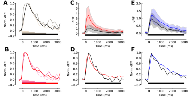
Figure 4: Blocking GABAergic transmission in the honeybee changes amplitude but not duration of the KC population response. (A) Temporal response profile of the Ca signal imaged in the mushroom body lip region of one honeybee for different stimulus durations as indicated by color. (B) Temporal response profiles as in (A) in one honeybee after application of PTX. (C) Response profiles imaged from 6 control animals (gray) and their average (black) for a 3s stimulus as indicated by the stimulus bar. The responses measured in 6 animals in which GABA_A transmission was blocked with PTX (red) shows a considerably higher population response amplitude. The shaded area indicated the standard deviation of responses across bees. (D) Average amplitude-normalized responses are highly similar in animals treated with PTX and control animals. (E) Blocking GABA_B transmission with CGP in 6 animals (blue) again results in an increased response amplitude compared to 6 control animals (black). The shaded area indicates the standard deviation across individuals. (F) Average normalized response profiles are highly similar in the CGP-treated and control animals.

To explore whether neuronal adaptation could be the responsible mechanism for temporal sparseness in the biological network, we performed a set of Calcium imaging experiments, monitoring Calcium responses in the KC population of the honeybee mushroom body[43] (Materials and Methods). Our computational model (Figure 3) predicted that blocking of the inhibitory microcircuit would increase the population response amplitude but should not alter the temporal dynamics of the KC population response. In a set of experiments, we tested this hypothesis by comparison of the KCs’ evoked activity in the presence and absence of GABAergic inhibition (Materials and Methods). First, we analyzed the normalized Calcium response signal within the mushroom body lip region in response to a 3s, 2s, 1s and 0.5s odor stimulus (Figure 4A). We observed the same brief phasic response following stimulus onset in all four cases with a characteristic slope of Calcium response decay that has been reported previously[43]. Bath application of the GABA_A antagonist picrotoxin (PTX) did not change the time course of the Calcium response dynamics (Figure 4B-D). The effectiveness of the drug was verified by the increased population response amplitude in initial phase (Figure 4C). Next, we tested the GABA_B antagonist hydrochloride (CGP) using the same protocol and again found an increase in the response magnitude but no alteration of the response dynamics (Figure 4E,F).

DISCUSSION

We here propose that a simple neuron-intrinsic mechanism of spike-triggered adaptation can account for a reliable and temporally sparse sensory stimulus representation across stages of sensory processing. At the single neuron level SFA is known to induce the functional property of a fractional differentiation with respect to the temporal profile of the input and thus offers the possibility of tuning the neuron’s response properties to the relevant stimulus time-scales at the cellular level[4, 3, 25]. Our results indicate that a sensory processing in a feedforeward network with adaptive neurons focuses on the temporal changes of the sensory input in a precise and temporally sparse manner (Figure 1B; Figure 2E and Figure 3E). At the same time the constancy of the stimulus is memorized in the cellular level of adaptation[32] (Figure 1D). We hypothesize that at later processing stages in the sensory pathway, notably in the sensory cortices and in the insect mushroom body, it is most relevant to encode and process relevant dynamic changes in the sensory environment and to neglect the static stimulus features as well as the dynamic fluctuations of receptor sensations present at very fast time scales. One prominent example is primate vision where, in the absence of the self-generated dynamics of retina input due to microsaccades, observers become functionally blind to stationary objects during fixations[26].

The emergence of a sparse representation has been demonstrated in various cortical sensory areas, for example in visual[44], auditory[14], somatosensory[16], and olfactory[35] cortices, and thus manifests a principle of sensory computation across sensory modalities and independent of the natural stimulus kinetic. However, it has been repeatedly questioned whether a few informative spikes can survive in the cortical network, which is highly sensitive to small perturbations[50, 24]. Our results show that a biologically realistic cellular mechanism implemented at successive network stages can transform a dense and highly variable Poisson input at the periphery into a sparse and highly reliable ensemble representation in the cortical network. These results reflect previous theoretical evidence that SFA has an extensive synchronizing-desynchronizing effect on population responses in a balanced network[46]. However, cellular adaptation has largely been neglected in theory and simulation of cortical networks, with very few exceptions[46], although it facilitates a transition from a dense rate code to a temporal code expressed in the concerted spiking of cortical cell assemblies[21] (Figure 2D).

Importantly, the adaption level adjusts with a dynamics that is slow compared to the dynamics of excitatoary and inhibitory synaptic inputs. This circumstance allows for a transient mismatch of the balanced state in the cortical network and thus leads to a transient reduction of the self-generated (recurrent) noise (Figure 2I). This, in turn, explains why the temporally sparse representation can be highly reliable. This result seems counter-intuitive in the light of previous studies that consistently stressed the persistence of noise in the balanced network[23, 28, 24]. However, cellular adaptation has largely been neglected in theory and simulation of cortical networks with very few exceptions[46].

Our results provide an understanding of the role of slow cellular adaptation dynamics for the transient suppression of the trial-by-trial response variability. We thus arrived at a coherent model explanation for the previously unexplained and wide-spread experimental phenomenon of a stimulus-driven transient reduction of response variability in cortical neurons, which has been observed in different species and across many cortical areas, from occipital to frontal, as e.g. reported by Churchland and colleagues for 14 independent datasets[9].

The insect olfactory system is experimentally well investigated and examplifies a pronounced sparse coding scheme at the level of the mushroom body KCs. The olfactory system is analog in invertebrates and vertebrates and the sparse stimulus representation is likewise observed in the pyramidal cells of the piriform cortex[35], and the rapid responses in the mitral cells in the olfactory bulb[40] compare to those of projection neurons in antennal lobe[19]. Our adaptive network model, designed in coarse analogy to the insect olfactory system, produced increasingly phasic population responses as the stimulus-driven acitivty propagated through the network. Our model results closely match the repeated experimental observation of temporally sparse KC responses in extracellular recordings from the locust[34] and manduca[6, 15], and in Calcium imaging in the honeybee[43].

In our experiments we could show that systemic blocking of GABAergic transmission did not affect the temporal sparseness of the KC population response in the honeybee (Figure 4). This result might seem to contradict former studies that stressed the role of inhibitory feed-forward[2] or feedback inhibition[33, 13] for the emergence of KC sparseness. However, the suggested inhibitory mechanisms and the sequential effect in the adaptive network proposed here are not mutually exclusive and may act in concert to establish and maintain a temporal and spatial sparse code in a rich and dynamic natural olfactory scene.

The adaptive network model manifests a low trial-to-trial variability of the sparse KC responses that typically consist of only 1-2 spikes. In consequence, a sparsly activated KC ensemble is able to robustly encode stimulus information. The low variability at the single cell level (Figure 3H) carries over to a low variability of the population response[11]. This benefits downstream processing in the mushroom body output neurons that integrate converging input from many KCs[27], and which were shown to reliably encode odor-reward associations in the honeybee[42].

Our results here bear consequences of general importance for sensory coding theories. A mechanism of self-inhibition at the cellular level can facilitate a temporally sparse ensemble code but does not require a well adjusted interplay between the excitatory and inhibitory circuitry at the network level. This network effect is robust due to the distributed nature of the underlying mechanism, which acts independently in each single neuron. The regularizing effect of self-inhibition increases the signal-to-noise ratio not only of single neuron responses but also of the neuronal population activity[11] that is postsynaptically integrated in downstream neurons.

Materials and Methods

Rate model of generic feedforward adaptive network

To address analytically the sequential effect of adaptation in a feedforward network, we consider a model in which populations are described by their firing rates. Although firing rate models typically provide a fairly accurate description of network behavior when the neurons are firing asynchronously[45], they do not capture all features of realistic networks. Therefore, we verify all of our predictions with a population density formalism[11] as well as a large-scale simulation of realistic spiking neurons. To determine the mean activity dynamics of a consecutive populations, we employed an standard mean firing rate model of population $i$ as

$$\begin{cases}\dot{r_{i}}=-r_{i}+f(gr_{i-1}+\mu_{i}-a_{i}|\sigma_{i})\\ \dot{a_{i}}=-\frac{1}{\tau_{s}}a_{i}+r_{i}q_{s}\end{cases}$$ (1)

where $f$ is the transfer input-output function, $\tau_{s}$ is the adaptation time-scale, $g$ is the coupling factor between two populations and $a$ is the adaptive negative feedback for the population $i$ with $q_{s}$ strength and $\sigma$ is the standard deviation of the input. For simplicity we define $m_{i}=gr_{i-1}+\mu_{i}$. Given $f$ the equilibrium can be determined by

$$\bar{r}_{i}=f(m_{i}-\tau_{s}q_{s}\bar{r}_{i}|\sigma_{i}).$$ (2)

This fix point is always stable[22] and the condition for the stability reads $\partial_{r_{i}}f(m-\tau_{s}q_{s}\bar{r}_{i}|\sigma_{i})|_{\bar{r}_{i}}<1$ and $\partial_{m_{i}}f(m-\tau_{s}q_{s}\bar{r}_{i}|\sigma_{i})|_{\bar{r}}<0$. It is also known that the $\bar{r}_{i}$ is a linear function, given a sufficiently slow adaptation $\tau_{s}$ and a non-linear shape of $f$ [10]. Thus, if $r_{i-1}=r_{i}$ in two subsequent populations, and increased input to population $i-1$ leads to smaller increase for next population $i$ and the adapted level of responses satisfy $\Delta r_{i-1}>\Delta r_{i}$.

The stimilus onset response lies between the adapted steady-state and not adapted responses function $f$ given the level of new input and can be analytical calculated accordingly[3].

Population density approach to the adaptive neuronal ensemble

In Muller et al.[29] it is shown that by an adiabatic elimination of fast variables a detailed neuron model including voltage dynamics, conductance-based synapses, and spike-induced adaptation reduces to a stochastic point process. Thus, we define an orderly point process with a hazard function argument with state variable $x$ as

$$h_{x}(x,t):=\lim_{\Delta t\rightarrow 0^{+}}\frac{\Pr(N[t,t+\Delta t)>0|x,t)}{\Delta t}.$$ (3)

where $N[t,t+\Delta t)$ is the number of events in $\Delta t$. We assume the dynamic of the adaptation variable is

$$\dot{x}=-\frac{1}{\tau_{s}}x+\sum_{k}\delta(t-t_{k})q_{s},$$ (4)

where $t_{k}$ is the time of $k$th spike in the ensemble. Thus, the state variable distribution at time $t$ in the ensemble is governed by a master equation of the form

$$\partial_{t}\Pr(x,t) = -\partial_{x}\left[\frac{x}{\tau_{s}}\Pr(x,t)\right]+h_{x}(x-q_{s},t)\Pr(x-q_{s},t)$$ (5)

$$- h_{x}(x,t)\Pr(x,t).$$

We solve the Eq. 5 with the help of the transformations $t_{s}=\eta(x):=-\tau\log(x/q)$ and $\psi(t_{s})=\eta(\eta^{-1}(t_{s}+q))$ numerically[29]. It turns out that indeed $h_{x}$ is the input-out transfer function of neurons in the network where its instantaneous parameters are give by the input statistics[29]. Here, we used the mean-field formalism developed by Lechner et al.[23] to approximately determine the averaged input within a standard balanced network, as the parameters of the hazard function $h_{x}$. Therefore, the functional form of its solution in a compact form is

$${\Pr}(t_{s}|t)=k_{t}\Omega(t_{s}|t)$$ (6)

where $t_{s}^{0}$ is the initial condition state of the system and $k_{t}$ is a constant defined by $\int{\Pr}(t_{s}|t)dt_{s}=1$. Hence, it can be shown that the firing rate and the consistency equation of the ensemble is

$$r_{t}=\int_{-\infty}^{\infty}h_{t_{s}}(t_{s}|t){\Pr}(t_{s}|t)dt_{s}.$$ (7)

Now, by applying the techniques in Farkhooi et al[11], we define a joint probability density as

$$\rho_{n}(t_{n},t_{x}^{n}|t_{x}^{0},t)$$ (8)

where an $n^{\mathrm{th}}$ event occurs at time $t_{n}>t$ and the state variable is $t_{x}^{n}$. We can write $n+1^{\mathrm{th}}$ event time and state of adaptation joint density recursively

$$\rho_{n+1}(t_{n+1},t_{x}^{n+1}|t_{x}^{0},t)=\int\int\rho(t_{n+1}-t_{n},t_{x}^{n+1}|t_{x}^{n},t)\rho_{n}(t_{n},t_{x}^{n}|t_{x}^{0},t)dt_{n}dt_{x}^{n}$$ (9)

To simplify the integral equations, we use Bra-Ket notation and thereafter, we derive the Laplace transform of the joint density by

$$\tilde{\rho}_{n+1}(s,t_{x}^{n+1}|t_{s}^{0},t)=\tilde{\rho}_{n}(s,t_{x}^{n}|t_{x}^{0},t)|\tilde{\rho}(s,t_{x}^{n+1}|t_{x}^{n},t)\rangle$$ (10)

where $\rho_{1}(t_{1},t_{s}^{1}|t_{x}^{0},t)=\rho(t_{1},t_{x}^{1}|t_{x}^{0},t)$ Next, we define the operator $\mathbf{P}_{n}(s|t)$,

$$\tilde{\rho}_{n}(s|t)=\langle 1\mid\mathbf{P}_{n}(s|t)\mid{\Pr}(t_{s},t)\rangle=\langle 1\mid\mathbf{P}^{n}(s|t)\mid{\Pr}(t_{x},t)\rangle.$$ (11)

Now, by employing $\tilde{P}(1,s|t)=1/(\mu_{1}s^{2})[\tilde{\rho}_{2}(s|t)-2\tilde{\rho}_{1}(s|t)+1]$ as in [11], we derive

$$\tilde{P}(n,s|t)=1/(\mu_{1}s^{2})[\tilde{\rho}_{n+1}(s|t)-2\tilde{\rho}_{n}(s|t)+\tilde{\rho}_{n-1}(s|t)],$$ (12)

where $\tilde{P}(n,s|t)$ is the Laplace transform of the probability density of observing $n$ events in a given time window. Now we derive

$$\textstyle\tilde{\mathcal{A}}_{s|t}=\sum_{k}\tilde{\rho}_{k}(s|t)=\langle 1\mid\mathbf{P}(s|t)/(\mathbf{I}-\mathbf{P}(s|t))\mid{\Pr}(s|t)\rangle$$ (13)

where $\mathbf{I}$ is the identity operator. This equation represents the Laplace transfom of the autocorrelation function. Thus, the Fano factor is $\tilde{J}_{s|t}=1/\mu_{1}s^{2}-(1+2\tilde{\mathcal{A}}_{s|t})$ and the inverse Laplace transform is

$$J_{T|t}=1+(2/T)\int_{0}^{T}(T-u)\mathcal{A}(u|t)du-Tr_{t},$$ (14)

where $\mathcal{A}(u|t)=\mathcal{L}^{-1}[\tilde{\mathcal{A}}_{s|t}]$.

Computational model of insect olfactory coding

Our model neuron is a general conductance-based integrate-and-fire neuron with spike-frequency adaptation as it is proposed in Muller et al.[29]. The model phenomenologically captures a wide array of biophysical spike-frequency mechanisms such as M-type current, afterhyperpolarization (AHP-current) and even slow recovery from inactivation of the fast sodium current[29]. The model neuron is also known to perform high-pass filtering of the input frequencies following the universal model of adaptation[3]. Neuron parameters used follow the Table.3 in Muller et al.[29] The conductance model used for the static synapses between the neurons is alpha-shaped with gamma distributed time constants from $\Gamma(2.5,4)$ and $\Gamma(5,4)$ for excitatory and inhibitory synapses, respectively. All simulations were performed using the NEST simulator[12] version 2.0beta and the Pynest interface.

The network connectivity is straight forward: each PN and LN receives excitatory connections from 20% randomly chosen OSNs[39, 8]. Additionally, every PN receives input from 50% randomly chosen inhibitory LNs[39, 8]. In our model the PNs do not excite one another and each PN output diverges to 50% randomly chosen KCs[43, 2, 17].

We tuned the simulated network by adjusting the synaptic weights to achieve the same spontaneous firing rate as reported experimentally: OSNs 15-25Hz[30], LNs 4-10Hz[8], PNs 3-10[19] and KCs   0.3-1.0Hz[15].

Experimental methods

Experiments were performed following the methods published in Szyszka et al[43]. In summary, foraging honeybees (Apis mellifera) were caught at the entrance of the hive, immobilized by chilling on ice, and fixed in a plexiglas chamber before the head capsule was opened for dye injection. We retrogradely stained clawed Kenyon cells (KC) of the median calyx, using the calcium sensor FURA-2 dextran (Molecular Probes, Eugene, USA) with a dye loaded glass electrode, which was pricked into KC axons projecting to the ventral median part of the $\alpha$-lobe[43]. After dye injection the head capsule was closed, bees feed and kept in a dark humid chamber for several hours.

The processing of imaging data was performed with custom written routines in IDL (RSI, Boulder, CO, USA). In summary, changes in the calcium concentration were measured as absolute changes of fluorescence: a ratio was calculated from the light intensities measured at 340nm and 380nm illumination and the background fluorescence before odor onset was subtracted leading to $\Delta$F with F = F340/F380. Odor stimulation was preformed under a 20x objective of the microscope, the naturally occurring plant odor octanol (Sigma Aldrich, Germany), diluted 1:100 in paraffine oil (FLUKA, Buchs, Switzerland), was delivered to both antennae of the bee using a computer controlled, custom made olfactometer. To this, odor loaded air was injected into a permanent airstream resulting in a further 1:10 dilution. Stimulus duration was 3 seconds if not mentioned otherwise. The air was permanently exhausted.

For GABA blockage, a solution of 150 $\mu$l GABA receptor antagonist dissolved in ringer for final concentration (10^-5M picrotoxin (PTX, Sigma Aldrich, Germany) or 5x10^-4M CGP54626 (CGP, Tocris Bioscience, USA)) was bath applied to the brain after pre-treatment measurements. Measurements started 10 min after drug application.

References

- 1. E. D. Adrian. The impulses produced by sensory nerve endings. The Journal of physiology, 61(1):49–72, 1926.
- 2. Collins Assisi, Mark Stopfer, Gilles Laurent, and Maxim Bazhenov. Adaptive regulation of sparseness by feedforward inhibition. Nat Neurosci, 10(9):1176–84, September 2007.
- 3. Jan Benda and Andreas V. M. Herz. A universal model for spike-frequency adaptation. Neural Computation, 15(11):2523–2564, November 2003.
- 4. Jan Benda, Andre Longtin, and Len Maler. Spike-frequency adaptation separates transient communication signals from background oscillations. J. Neurosci., 25(9):2312–2321, March 2005.
- 5. Jan Benda, Leonard Maler, and André Longtin. Linear versus nonlinear signal transmission in neuron models with adaptation currents or dynamic thresholds. Journal of Neurophysiology, 104(5):2806 –2820, November 2010.
- 6. Bede M Broome, Vivek Jayaraman, and Gilles Laurent. Encoding and decoding of overlapping odor sequences. Neuron, 51(4):467–82, August 2006.
- 7. Maurice J. Chacron, Leonard Maler, and Joseph Bastian. Electroreceptor neuron dynamics shape information transmission. Nature Neuroscience, 8(5):673–678, 2005.
- 8. Ya-Hui Chou, Maria L Spletter, Emre Yaksi, Jonathan C S Leong, Rachel I Wilson, and Liqun Luo. Diversity and wiring variability of olfactory local interneurons in the drosophila antennal lobe. Nature Neuroscience, 13(4):439–449, February 2010.
- 9. Mark M Churchland, Byron M Yu, John P Cunningham, Leo P Sugrue, Marlene R Cohen, Greg S Corrado, William T Newsome, Andrew M Clark, Paymon Hosseini, Benjamin B Scott, David C Bradley, Matthew A Smith, Adam Kohn, J Anthony Movshon, Katherine M Armstrong, Tirin Moore, Steve W Chang, Lawrence H Snyder, Stephen G Lisberger, Nicholas J Priebe, Ian M Finn, David Ferster, Stephen I Ryu, Gopal Santhanam, Maneesh Sahani, and Krishna V Shenoy. Stimulus onset quenches neural variability: a widespread cortical phenomenon. Nat Neurosci, 13(3):369–378, March 2010.
- 10. B. Ermentrout. Linearization of FI curves by adaptation. Neural computation, 10(7):1721–1729, 1998.
- 11. Farzad Farkhooi, Eilif Muller, and Martin P. Nawrot. Adaptation reduces variability of the neuronal population code. Physical Review E, 83(5):050905, May 2011.
- 12. Marc-Oliver Gewaltig and Markus Diesmann. NEST (NEural simulation tool). Scholarpedia, 2(4):1430, 2007.
- 13. N. Gupta and M. Stopfer. Functional analysis of a higher olfactory center, the lateral horn. Journal of Neuroscience, 32(24):8138–8148, June 2012.
- 14. Tomáš Hromádka, Michael R DeWeese, and Anthony M Zador. Sparse representation of sounds in the unanesthetized auditory cortex. PLoS Biol, 6(1):e16, January 2008.
- 15. Iori Ito, Rose Chik-ying Ong, Baranidharan Raman, and Mark Stopfer. Sparse odor representation and olfactory learning. Nature Neuroscience, 11(10):1177–1184, September 2008.
- 16. Shantanu P Jadhav, Jason Wolfe, and Daniel E Feldman. Sparse temporal coding of elementary tactile features during active whisker sensation. Nature Neuroscience, 12(6):792–800, May 2009.
- 17. Ron A. Jortner, S. Sarah Farivar, and Gilles Laurent. A simple connectivity scheme for sparse coding in an olfactory system. The Journal of Neuroscience, 27(7):1659 –1669, February 2007.
- 18. Mikiko Kadohisa and Donald A. Wilson. Olfactory cortical adaptation facilitates detection of odors against background. Journal of Neurophysiology, 95(3):1888–1896, March 2006.
- 19. Sabine Krofczik, Randolf Menzel, and Martin P. Nawrot. Rapid odor processing in the honeybee antennal lobe network. Frontiers in Computational Neuroscience, 2, 2008. PMID: 19221584 PMCID: 2636688.
- 20. A. Kumar, S. Schrader, A. Aertsen, and S. Rotter. The high-conductance state of cortical networks. Neural Computation, 20(1):1–43, 2008.
- 21. Arvind Kumar, Stefan Rotter, and Ad Aertsen. Spiking activity propagation in neuronal networks: reconciling different perspectives on neural coding. Nat Rev Neurosci, 11(9):615–627, 2010.
- 22. Giancarlo LaCamera, Alexander Rauch, Hans-R Luscher, Walter Senn, and Stefano Fusi. Minimal models of adapted neuronal response to in vivo-like input currents. Neural Comput, 16(10):2101–2124, October 2004.
- 23. Alexander Lerchner, Cristina Ursta, John Hertz, Mandana Ahmadi, Pauline Ruffiot, and Søren Enemark. Response variability in balanced cortical networks. Neural Computation, 18(3):634–659, 2006.
- 24. Michael London, Arnd Roth, Lisa Beeren, Michael Hausser, and Peter E. Latham. Sensitivity to perturbations in vivo implies high noise and suggests rate coding in cortex. Nature, 466(7302):123–127, July 2010.
- 25. Brian N. Lundstrom, Matthew H. Higgs, William J. Spain, and Adrienne L. Fairhall. Fractional differentiation by neocortical pyramidal neurons. Nature Neuroscience, 11(11):1335–1342, 2008.
- 26. Susana Martinez-Conde, Stephen L. Macknik, Xoana G. Troncoso, and David H. Hubel. Microsaccades: a neurophysiological analysis. Trends in Neurosciences, 32(9):463–475, September 2009.
- 27. R. Menzel and Larry R. Squire. Olfaction in invertebrates: Honeybee. In Encyclopedia of Neuroscience, pages 43–48. Academic Press, Oxford, 2009.
- 28. Michael Monteforte and Fred Wolf. Dynamical entropy production in spiking neuron networks in the balanced state. Physical Review Letters, 105(26):268104, December 2010.
- 29. Eilif Muller, Lars Buesing, Johannes Schemmel, and Karlheinz Meier. Spike-frequency adapting neural ensembles: Beyond mean adaptation and renewal theories. Neural Comp., 19(11):2958–3010, 2007.
- 30. Katherine I Nagel and Rachel I Wilson. Biophysical mechanisms underlying olfactory receptor neuron dynamics. Nature Neuroscience, 14(2):208–216, January 2011.
- 31. Martin P. Nawrot, Clemens Boucsein, Victor Rodriguez Molina, Alexa Riehle, Ad Aertsen, and Stefan Rotter. Measurement of variability dynamics in cortical spike trains. Journal of Neuroscience Methods, 169(2):374–390, April 2008.
- 32. William H. Nesse, Leonard Maler, and André Longtin. Biophysical information representation in temporally correlated spike trains. Proceedings of the National Academy of Sciences, 107(51):21973 –21978, December 2010.
- 33. Maria Papadopoulou, Stijn Cassenaer, Thomas Nowotny, and Gilles Laurent. Normalization for sparse encoding of odors by a wide-field interneuron. Science, 332(6030):721 –725, May 2011.
- 34. Javier Perez-Orive, Ofer Mazor, Glenn C Turner, Stijn Cassenaer, Rachel I Wilson, and Gilles Laurent. Oscillations and sparsening of odor representations in the mushroom body. Science, 297(5580):359–65, July 2002.
- 35. Cindy Poo and Jeffry S. Isaacson. Odor representations in olfactory cortex: “Sparse” coding, global inhibition, and oscillations. Neuron, 62(6):850–861, June 2009.
- 36. R. Ranganathan. Evolutionary origins of ion channels. Proceedings of the National Academy of Sciences of the United States of America, 91(9):3484, 1994.
- 37. Alex Roxin, Nicolas Brunel, David Hansel, Gianluigi Mongillo, and Carl van Vreeswijk. On the distribution of firing rates in networks of cortical neurons. The Journal of Neuroscience, 31(45):16217 –16226, November 2011.
- 38. B. Rudy. Diversity and ubiquity of k channels. Neuroscience, 25(3):729–749, June 1988.
- 39. Silke Sachse and C. Giovanni Galizia. Role of inhibition for temporal and spatial odor representation in olfactory output neurons: A calcium imaging study. J Neurophysiol, 87(2):1106–1117, February 2002.
- 40. Roman Shusterman, Matthew C Smear, Alexei A Koulakov, and Dmitry Rinberg. Precise olfactory responses tile the sniff cycle. Nature Neuroscience, 14(8):1039–1044, July 2011.
- 41. Richard B. Stein, E. Roderich Gossen, and Kelvin E. Jones. Neuronal variability: noise or part of the signal? Nat Rev Neurosci, 6(5):389–397, May 2005.
- 42. Martin Fritz Strube-Bloss, Martin Paul Nawrot, and Randolf Menzel. Mushroom body output neurons encode odor-reward associations. J. Neurosci., 31(8):3129–3140, February 2011.
- 43. Paul Szyszka, Mathias Ditzen, Alexander Galkin, C. Giovanni Galizia, and Randolf Menzel. Sparsening and temporal sharpening of olfactory representations in the honeybee mushroom bodies. Journal of Neurophysiology, 94(5):3303 –3313, November 2005.
- 44. David J. Tolhurst, Darragh Smyth, and Ian D. Thompson. The sparseness of neuronal responses in ferret primary visual cortex. The Journal of Neuroscience, 29(8):2355 –2370, February 2009.
- 45. A. Treves. Mean-field analysis of neuronal spike dynamics. Network: Computation in Neural Systems, 4(3):259–284, 1993.
- 46. C. van Vreeswijk. Analysis of the asynchronous state in networks of strongly coupled oscillators. Phys Rev Lett, 84(22):5110–5113, May 2000.
- 47. C. van Vreeswijk and H. Sompolinsky. Chaotic balanced state in a model of cortical circuits. Neural Comput, 10(6):1321–71, August 1998.
- 48. Tim P Vogels and L F Abbott. Gating multiple signals through detailed balance of excitation and inhibition in spiking networks. Nat Neurosci, 12(4):483–491, April 2009.
- 49. Barry Wark, Brian Nils Lundstrom, and Adrienne Fairhall. Sensory adaptation. Current opinion in neurobiology, 17(4):423–429, August 2007. PMID: 17714934 PMCID: PMC2084204.
- 50. Jason Wolfe, Arthur R Houweling, and Michael Brecht. Sparse and powerful cortical spikes. Current Opinion in Neurobiology, 20(3):306–312, June 2010.