Using controlled disorder to distinguish $s_{\pm}$ and $s_{++}$ gap structure in Fe-based superconductors

Abstract

We reconsider the effect of disorder on the properties of a superconductor characterized by a sign-changing order parameter appropriate for Fe-based materials. Within a simple two band model, we calculate simultaneously $T_{c}$, the change in residual resistivity $\Delta\rho_{0}$, and the zero-energy density of states, and show how these results change for various types of gap structure and assumptions regarding the impurity scattering. The rate of $T_{c}$ suppression is shown to vary dramatically according to details of the impurity model considered. We search therefore for a practical, experimentally oriented signature of a gap of the $s_{\pm}$ type, and propose that observation of a particular evolution of the penetration depth, nuclear magnetic resonance relaxation rate, or thermal conductivity temperature dependence with disorder would suffice.

I Introduction

Determining the symmetry and structure of the superconducting order parameter in iron-based superconductors (FeSCs) is one of the main challenges in this new field. Hirschfeld_rev11 ; *Chubukov12 The Fermi surface is usually given by two or three $[\Gamma\!=\!(0,0)]$-centered hole pockets and two $[M\!=\!(\pi,\pi)]$-centered electron pockets in the two-Fe zone composed primarily of Fe $3d$ states. Repulsive interband interactions between hole and electron pockets leading to spin fluctuations are often assumed to lead to a superconducting order parameter which changes sign over the Fermi surface (FS) to lower the overall Coulomb energy. The simplest version of this state, called the $s_{\pm}$ state, is described by an isotropic order parameter on each FS with opposite signs for electronlike and holelike pockets. Mazin08 The state may be highly anisotropic and even exhibit gap nodes, but still be considered $s_{\pm}$ provided the average sign on hole pockets is opposite that on electron pockets. On the other hand, other theories suggest that orbital fluctuations may dominate the pairing interactions in systems of this type, favoring a gap with equal sign on all pockets, denoted $s_{++}$. Kontani10

Surprisingly, it has proven rather difficult to definitively distinguish these types of gap structures experimentally, in part because phase-sensitive experiments are challenging due to surface properties; because of the multiband nature of the electronic structure; and because the $s_{\pm}$ and $s_{++}$ “states” are symmetry equivalent, transforming both according to the $A_{1g}$ representation of the crystal point group. At this writing, three experiments offer indirect evidence in favor of the $s_{\pm}$ state: the nearly ubiquitous observation of neutron spin resonance features in inelastic neutron spectroscopy (INS), Lumsden09 ; Christianson09 ; Inosov10 ; Park10 ; Argyriou10 ; Castellan11 a quasiparticle interference scanning tunneling spectroscopy (STS) experiment in a magnetic field, Hanaguri10 and a phase-sensitive experiment on a polycrystalline sample which relies on significant statistical analysis. Chen10

On the other hand, alternative explanations have been offered for all these measurements; in particular, Kontani and Onari have provided an alternate explanation Kontani10 for the neutron resonance features within an $s_{++}$ scenario via a postulated energy dependence of the quasiparticle relaxation time. In addition, several references Senga08 ; Senga09 ; Onari09 ; Lietal12 ; Kirshenbaum12 have called attention to a “slow” decrease of $T_{c}$ in chemical substitution experiments, Li10 ; Nakajima10 ; Tropeano10 ; Lietal12 ; Kirshenbaum12 which is then ascribed to the natural robustness against nonmagnetic disorder of an $s_{++}$ superconductor. It is this issue which we study here.

It is important to understand what is meant by “slow” and “fast” $T_{c}$ suppression in this context. At one extreme we have situations in which $T_{c}$ is not suppressed by nonmagnetic disorder at all. According to Anderson’s theorem, the critical temperature of an isotropic conventional $s$-wave superconductor with a single band of electrons is unaffected by nonmagnetic scatterers. From this statement it follows immediately that the same occurs for two bands in an isotropic $s_{++}$ state (with equal gaps), but also in an $s_{\pm}$ state with no interband scattering. At the other extreme, we know that magnetic scatterers in a conventional isotropic superconductor suppress $T_{c}$ according to the Abrikosov-Gor’kov (AG) law; Abrikosov61 it is well known that nonmagnetic scatterers suppress $T_{c}$ at the same fast AG rate in a two-band $s_{\pm}$ state, provided the two densities of states $N_{a}=N_{b}$ and two gaps $\Delta_{a}=-\Delta_{b}$ are equal in magnitude, and the scattering is purely interband in nature. Any deviation from these assumptions will slow the $T_{c}$ suppression rate relative to the AG rate. Therefore between these two extremes lie many possibilities for $T_{c}$ suppression behavior which depend on details of the electronic structure and the relative amplitudes of inter- and intraband scattering.

Several theoretical calculations of $T_{c}$ suppression have discussed the pairbreaking effects of nonmagnetic scatterers on model multiband superconductors with generalized $s$-wave order. Preosti96 ; Golubov97 ; *Golubov95; Parker08 ; Chubukov08 ; Senga08 ; *Senga09; Bang09 ; Mishra09 ; Golubov02 ; Kogan09 ; Kulic99 ; *Ohashi04; Efremov11 In fact the situation is generally even more complicated than discussed above or in these works, since chemical impurities may do more than simply provide a scattering potential: they may dope the system, or alter the pairing interaction itself locally. We therefore believe (see also Ref. Hirschfeld_rev11, ; *Chubukov12) that measurements of $T_{c}$ suppression relative to the amount of chemical disorder are not particularly useful to determine the gap structure in multiband systems. To improve the situation, one first needs to find a way to create pointlike potential scattering centers, so as to create disordered systems to which the above theoretical works apply. The closest approach to this ideal is achieved with low-energy electron irradiation, which is thought to create interstitial-vacancy pairs. Experiments of this type are being performed currently, and it is one of the goals of this work to make predictions to guide the analysis of such data.

The other needed improvements are theoretical: first, the pairbreaking theory must be extended to relate $T_{c}$ only to directly measurable quantities, like the change in residual ($T\rightarrow 0$) resistivity caused by the disorder, rather than to any theoretically meaningful but empirically inaccessible scattering rate parameter. Second, since the theory involves many parameters, the robustness of any claimed fit must be tested by the simultaneous prediction of other quantities which depend on disorder, such as the low-temperature penetration depth, nuclear magnetic resonance (NMR) relaxation rate, or thermal conductivity. Finally, it would be useful to have ab initio calculations of vacancy and interstitial potentials to constrain the impurity parameters used. This has been attempted for chemical substituents Kemper09 ; *Kemper10_erratum; Nakamura11 recently.

II Model

We consider a system with two bands $a$ and $b$ with linearized dispersion close to the Fermi level that lead to densities of state $N_{a}$ and $N_{b}$ in the normal state; see Fig. 1.

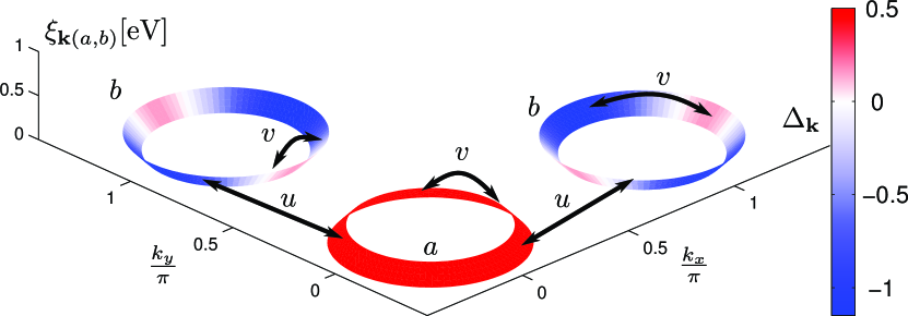
Figure 1: (Color online) Sketch of the two-band model with linearized band dispersions on the Fermi sheets $a$ and $b$ and constant impurity scattering $v$ (intraband) and $u$ (interband), together with a possible nodal $s$-wave gap on the bands in the superconducting state.

The $t$-matrix equation in the two-band model has the form

$$\mathbf{\hat{\Sigma}} = {n}_{\text{imp}}\mathbf{\hat{t}},$$ (1a)

$$\mathbf{\hat{t}} = \mathbf{\hat{u}}+\mathbf{\hat{u}\hat{g}}\mathbf{\hat{t}},$$ (1b)

where $n_{\mathrm{imp}}$ is the concentration of impurities, $\mathbf{\hat{t}}(n_{\mathrm{imp}})=\sum_{i=0}^{3}\mathbf{t}^{(i)}\mathbf{\otimes}\hat{\tau}_{i}$, $\mathbf{\hat{g}}(n_{\mathrm{imp}})=\mathbf{g}_{0}\mathbf{\otimes}\hat{\tau}_{0}+\mathbf{g}_{1}\mathbf{\otimes}\hat{\tau}_{1}$ and $\mathbf{\otimes}$ represents a product of band (bold) and Nambu (caret) matrices. $\mathbf{g}_{0}=\mathop{\mathrm{missing}}{diag}(g_{0a},g_{0b})$ and $\mathbf{g}_{1}=\mathop{\mathrm{missing}}{diag}(g_{1a},g_{1b})$ are local Green’s functions in the $\tau_{0}$ and $\tau_{1}$ channels (we have assumed particle-hole symmetry in order to neglect $\mathbf{g}_{3}$), where $\hat{\tau}_{i}$ denote Pauli matrices in Nambu space. Due to the translational invariance of the disorder-averaged system, $\mathbf{\hat{g}}$ is diagonal in band space. We now assume a simple model for impurity scattering whereby electrons scatter within each band with amplitude $v$ and between bands with amplitude $u$,

$$\hat{{\bf u}}=\left(\begin{array}[]{cc}v&u\\ u&v\end{array}\right)\mathbf{\otimes}\hat{\tau}_{3}.$$ (2)

The $t$-matrix components are found from Eq. (1b) to be

$$t_{aa}^{(0)} = \frac{\left[g_{0b}u^{2}+g_{0a}v^{2}-g_{0a}\left(u^{2}-v^{2}\right)^{2}\delta g_{b}^{2}\right]}{\mathcal{D}},$$

$$t_{aa}^{(1)} = -\frac{\left[g_{1b}u^{2}+g_{1a}v^{2}-g_{1a}\left(u^{2}-v^{2}\right)^{2}\delta g_{b}^{2}\right]}{\mathcal{D}},$$ (3)

and $t_{bb}^{(i)}=t_{aa}^{(i)}(a\leftrightarrow b)$, where

$${\mathcal{D}} = 1-\left(\delta g_{a}^{2}+\delta g_{b}^{2}\right)v^{2}+\delta g_{a}^{2}\delta g_{b}^{2}\left(u^{2}-v^{2}\right)^{2}-$$ (4)

$$-2u^{2}\left(g_{0a}g_{0b}-g_{1a}g_{1b}\right)$$

with the abbreviation $\delta g_{\alpha}^{2}=g_{0\alpha}^{2}-g_{1\alpha}^{2}$.

III $T_{c}$ suppression

The linearized multiband gap equation near $T_{c}$ is (see, e.g. Ref. Mishra09, )

$$\Delta_{\alpha}{(\mathbf{k})}=2T\!\sum_{{\bf k}^{\prime},\beta,\omega_{n}>0}^{\omega_{n}=\omega_{c}}\!V^{\alpha\beta}_{{\bf k}{\bf k}^{\prime}}\frac{\tilde{\Delta}_{\beta}({\bf k}^{\prime})}{\tilde{\omega}^{2}_{\beta}+\xi^{2}_{\beta}},$$ (5)

where $\xi_{\beta}$ is the linearized dispersion of band $\beta$, and we introduced the shifted gaps and frequencies, $\tilde{\Delta}_{\beta}({\bf k}^{\prime})={\Delta}_{\beta}({\bf k}^{\prime})+\Sigma_{\beta}^{(1)}$ and ${\tilde{\omega}_{\beta}}=\omega_{n}+{i\Sigma_{\beta}^{(0)}}$. We will simplify the model above further in that we adopt a gap structure similar to that obtained from spin fluctuation theories: The gap on the (hole) pocket $a$ is isotropic, $\Delta_{a}$, and the gap on the (electron) pocket $b$ may be anisotropic, $\Delta_{b}=\Delta_{b}^{0}+\Delta_{b}^{1}(\theta)$, where $\theta$ is the momentum angle around the $b$ pocket and $\int d\theta\Delta_{b}^{1}(\theta)=0$. The pairing potential is then taken as $V^{\alpha\beta}_{{\mathbf{k}}{\mathbf{k}}^{\prime}}=V_{\alpha\beta}\phi_{\alpha}({\mathbf{k}})\phi_{\beta}({\mathbf{k}}^{\prime})$, with $\phi_{\alpha}=1+r\delta_{\alpha,b}\cos 2\phi$, and $\phi$ is the angle around the electron pocket. The parameter $r$ controls the degree of anisotropy, and creates nodes if $r>1$.

This ansatz then gives three coupled gap equations for $(\Delta_{a},\Delta_{b}^{0},\Delta_{b}^{1})^{\text{T}}\equiv\underline{\Delta}$. In the $\underline{\Delta}$ basis we can write the gap equations in the compact form

$$\underline{\Delta}={\ln}\Bigl{(}1.13\frac{\omega_{c}}{T_{c}}\Bigr{)}\underline{\mathcal{M}}\,\underline{\Delta}{\equiv\mathcal{L}_{0}\underline{\mathcal{M}}\,\underline{\Delta}},$$ (6)

the matrix $\underline{\mathcal{M}}=({1}+\underline{V}\,\underline{\mathcal{R}}^{-1}\underline{\mathcal{X}}\,\underline{\mathcal{R}})^{-1}\,\underline{V}$ and the constant $\mathcal{L}_{0}=\ln\bigl{(}1.13\frac{\omega_{c}}{T_{c}}\bigr{)}$ were introduced. Here $\underline{V}$ is the interaction matrix in the above basis. $\underline{\mathcal{R}}$ is the orthogonal matrix which diagonalizes the matrix $\underline{\Lambda}$,

$$\underline{\Lambda}=\frac{\pi n_{\text{imp}}}{\mathcal{D}_{N}}\left[\begin{array}[]{ccc}N_{b}u^{2}&{-}N_{b}u^{2}&0\\ {-}N_{a}u^{2}&N_{a}u^{2}&0\\ 0&0&{N_{b}v^{2}+N_{a}u^{2}}\\ \end{array}\right],$$ (7)

where

$$\mathcal{D}_{N}=1+2u^{2}\pi^{2}N_{a}N_{b}+(u^{2}-v^{2})^{2}\pi^{4}N_{a}^{2}N_{b}^{2}+v^{2}\pi^{2}(N_{a}^{2}+N_{b}^{2})$$ (8)

is Eq. (4) evaluated in the normal state where the limit $\underline{\Delta}\rightarrow 0$ has been taken in the local Greens functions. $\underline{\mathcal{X}}$ is a matrix with only diagonal elements,

$${\mathcal{X}}_{ii}={\mathcal{L}_{0}-\left[\Psi\Bigl{(}\frac{1}{2}+\frac{\omega_{c}}{2\pi T_{c}}+\frac{\lambda_{i}}{2\pi T_{c}}\Bigr{)}-\Psi\Bigl{(}\frac{1}{2}+\frac{\lambda_{i}}{2\pi T_{c}}\Bigr{)}\right]},$$ (9)

where $\Psi$ is the digamma function and $\lambda_{i}$ are the eigenvalues of the matrix $\underline{\Lambda}$. The maximum eigenvalue $[\lambda_{\text{max}}(T_{c})]$ of the matrix $\underline{\mathcal{M}}$ determines $T_{c}$ via $T_{c}=1.13\;\omega_{c}\exp\left[-1/\lambda_{\text{max}}(T_{c})\right]$.

IV Residual resistivity

The most direct observable measure of scattering in $T_{c}$ suppression experiments is the residual resistivity change $\Delta\rho_{0}$, i.e., the change in the extrapolated $T\rightarrow 0$ value of the resistivity with disorder. We will assume that interference effects between elastic and inelastic processes are negligible, i.e., that the effect on the $\rho(T)$ curve when the system is disordered is essentially a $T$-independent shift upward. We therefore calculate $\Delta\rho_{0}$ within the same framework as above, assuming that all defects are pointlike. In the zero frequency limit, there are no interband transitions, and the total conductivity in the $x$ direction is the sum of the Drude conductivities of the two bands, $\sigma=\sigma_{a}+\sigma_{b},$ with $\sigma_{\alpha}=2e^{2}N_{\alpha}\langle v_{\alpha,x}^{2}\rangle\tau_{\alpha}$, where $v_{\alpha,x}$ is the component of the Fermi velocity in the $x$ direction and $\tau_{\alpha}$ the corresponding single particle relaxation time obtained from the self-energy in the $t$-matrix approximation, $\tau_{\alpha}^{-1}=-2\mathop{\mathrm{Im}}\Sigma_{\alpha}^{(0)}$. Note that $\tau_{\alpha}^{-1}$ contains contributions from both the intraband and interband impurity scattering processes. The transport time and single-particle lifetime are identical within this model because of our assumption of pointlike $s$-wave scatterers, which implies that corrections to the current vertex vanish. A finite spatial range of the scattering potential will tend to steepen the $T_{c}$ vs $\Delta\rho_{0}$ curve.Graser_forward ; Zhu04

V Results

V.1 $T_{c}$ suppression vs resistivity

We now solve Eqs. (6) for $T_{c}$ and calculate simultaneously the change in resistivity $\Delta\rho_{0}$ at $T\rightarrow 0$. Unlike $T_{c}$ vs $n_{\mathrm{imp}}$ or various scattering rates, $T_{c}$ vs $\Delta\rho_{0}$ can then be compared directly to experiment. Clearly, the results will be parameter dependent, however, so we here specify our precise assumptions regarding the electronic structure. For concreteness, we focus on the BaFe₂As₂ (Ba122) system on which the largest number of measurements have been reported, and give parameters for this system and corresponding references in the Appendix.

Using these parameters, we obtain for the isotropic case ($r=0$) the zero temperature gap values of $\Delta_{a0}^{0}=-1.79T_{c0}$ and $\Delta_{b0}^{0}=1.73T_{c0}$, whereas for the nodal case ($r=1.3$) these are $\Delta_{a0}^{0}=-1.22T_{c0}$ and $\Delta_{b0}^{0}=1.23T_{c0}$ with the critical temperature chosen as $T_{c0}=30$ K. We have fixed the intraband scattering potential at an intermediate strength value of $v=0.25$, but show results for other values in the Appendix. Potentials are given in eV and we set $\hbar=k_{\text{B}}=1$.

In Fig. 2, we now exhibit $T_{c}$ suppression vs the corresponding change in residual resistivity $\Delta\rho_{0}$ as defined above, both for a fully isotropic $s_{\pm}$ gap ($r=0$), and for a gap which has nodes on the electron pockets ($r=1.3$), for a range of ratios $u/v$. It is clear that a wide variety of initial slopes and critical resistivities $\Delta\rho_{0}^{c}$ for which $T_{c}\rightarrow 0$ is possible, depending on the scattering character of the impurity. The variability of the suppression rate with the ratio of inter- to intraband scattering has been noted by various authorsMishra09 ; Efremov11 before this. In fact, Efremov et al.Efremov11 have shown that the various $T_{c}$ suppression curves of the isotropic $s_{\pm}$ gap fall onto universal curves depending on whether the average pair coupling constant $\langle\lambda\rangle<,=,>0$ when plotted against the interband scattering rate (which is not directly measurable, however). Other works have made comparisons with the resistivity changes (for example Refs. Lietal12, ; Kirshenbaum12, ), but have typically presented results for $s_{\pm}$ states only for a single set of impurity parameters corresponding to the fastest rate of $T_{c}$ suppression. Such assumptions lead always to critical $\Delta\rho_{0}$’s comparable to the smallest ones seen in Fig. 2, of order tens of $\mu\Omega$ cm. Here we see that more general values of the parameters can easily lead to much slower $T_{c}$ vs $\Delta\rho_{0}$ suppression rates by disorder, with critical disorder values of $\Delta\rho_{0}^{c}$ of order m$\Omega$ cm. As discussed by Li et al.,Lietal12 such values are typical of chemical substitutions on various different lattice sites; here we see that such slow $T_{c}$ suppression does not rule out the $s_{\pm}$ state, even within the assumptions of our potential-scattering-only model.

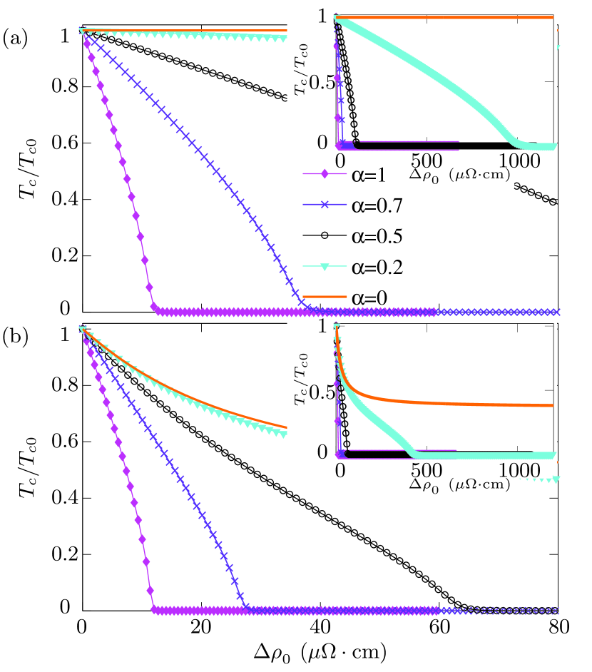
Figure 2: (Color online) (a) Normalized critical temperature $T_{c}/T_{c0}$ vs disorder-induced resistivity change $\Delta\rho_{0}$ for isotropic $s\pm$-wave pairing for various values of the inter- to intraband scattering ratio $\alpha\equiv u/v$. Inset: Same quantity plotted over a larger $\Delta\rho_{0}$ scale. (b) As (a) but for an anisotropic (nodal) gap with anisotropy parameter $r=1.3$.

V.2 Density of states

A real understanding of the effects of disorder in a given situation will probably depend on correlating the results of several experiments. Other quantities which are quite sensitive to disorder are the temperature dependence of the low-$T$ London penetration depth $\Delta\lambda(T)$ and the nuclear magnetic spin-lattice relaxation time $T_{1}^{-1}$. Within BCS theory, these quantities are controlled by the low-energy density of states. In the pure system, the nodal structure then determines the power law of temperature, and one generically expects $\Delta\lambda(T)\sim T$ for gap line nodes except in very special situations.Grossetal86 In the presence of a small amount of nonmagnetic disorder, a finite density of states is created GorkovKalugin ; RiceUeda which leads automatically to a $T^{2}$ term in the penetration depth.Grossetal86 ; felds If the state is of $s$ character, the gap nodes are not symmetry protected and can be lifted by further addition of disorder.Borkowski ; Mishra09

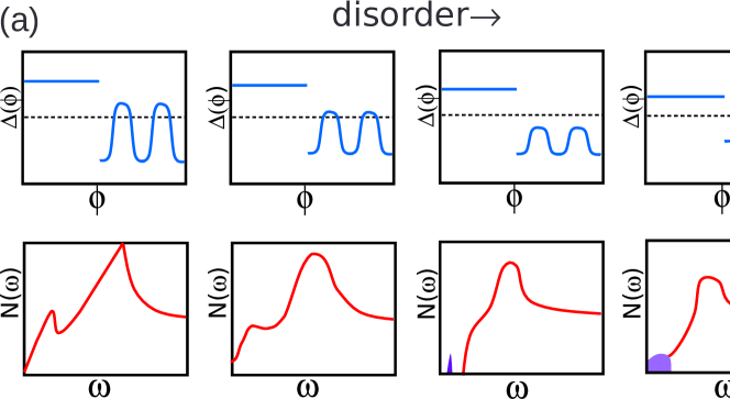
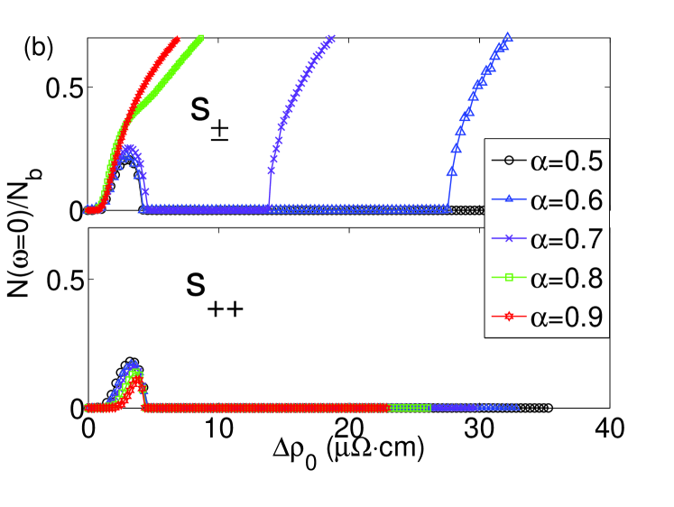
Figure 3: (Color online) (a) Schematic evolution of the order parameter and density of states with increasing disorder for a system with intra- and interband scattering. (b) Top: Fermi level density of states $N_{b}(0)$ (nodal band) as shown in Fig. 2(b) vs $\Delta\rho_{0}$ for various values of scattering ratio $u/v$ in an anisotropic $s_{\pm}$ state. Bottom: Fermi-level density of states for anisotropic $s_{++}$ state with $V_{ab}$ identical in magnitude to the above panel, but positive. Anisotropy parameter $r=1.3$ in both cases.

In this work we note a further possibility in the disorder evolution of the low-energy density of states (DOS) of a nodal multiband $s_{\pm}$-wave superconductor, namely, that a reentrant behavior of $N(0)$ can occur after lifting of the nodes. The reason is that, in a situation dominated by intraband scattering but with nonzero interband scattering, anisotropy of the gaps on each individual sheet will be averaged by intraband disorder quickly. If the state is $s_{\pm}$, a midgap impurity state can then be created by interband scattering, and grow until it overlaps the Fermi level, as shown schematically in Fig. 3 (a). Such midgap states are the analogs of the Yu-Shiba bound states created by magnetic impurities in conventional superconductors, and can appear for nonmagnetic impurities if the superconducting gap changes sign.balatskyRMP The residual density of states $N(0)=-\mathop{\mathrm{Im}}\sum_{\bf k}\mathop{\mathrm{Tr}}\hat{G}({\bf k},\omega=0)/(2\pi)$ ($\hat{G}$ is the Nambu Green’s function) effectively determines the low-energy thermodynamic behavior, so we have plotted it for the anisotropic band as a function of increasing disorder in Fig. 3, for both $s_{\pm}$ and $s_{++}$ states. In the former case the reentrant behavior is clearly seen.

The corresponding sequence in the $s_{\pm}$ penetration depth $\Delta\lambda(T)$ would be $T\rightarrow T^{2}\rightarrow\exp(-\Omega_{G}/T)\rightarrow T^{2}$, where $\Omega_{G}$ is the minimum gap in the system, while for the NMR spin-lattice relaxation rate $T_{1}^{-1}$, the analogous evolution should be $T^{3}\rightarrow T\rightarrow\exp(-\Omega_{G}/T)\rightarrow T$. The residual linear $T$ term in the thermal conductivity, $\kappa(T\rightarrow 0)/T$, should vanish and then reappear with increasing disorder. In the $s_{++}$ case, the last step in each sequence is entirely absent, since interband scattering cannot give rise to low-energy bound state formation.

V.3 Realistic impurity potentials

It is clear from the above analysis that we have established that there is a wide range of possibilities for the behavior of $T_{c}$ in an $s_{\pm}$ superconductor, as well as for low-temperature properties like the penetration depth, when disorder is systematically increased. To make more precise statements, one needs to have some independent way to fix the scattering potential of a given impurity, and in particular the relative proportion of inter- to intraband scattering. Kemper et al. Kemper09 found the ratio between inter- and intraband scattering to be of order $\alpha=0.3$ for Co in Ba122, which would lead according to Fig. 2 to a critical resistivity strength of about 300 $\mu\Omega$ cm, roughly in accord with experiment.Lietal12 ; Kirshenbaum12 Onari and KontaniOnari09 have made the important point that the “natural” formulation for a model impurity potential, i.e., diagonal in the basis of the five Fe $d$ orbitals, automatically leads to significant interband scattering if one transforms back to the band basis. However, simple estimates show that depending on details $\alpha$ for on-site Fe substituents can vary between 0.2 and 1, again leading as seen in Fig. 2 to a wide variety of possible $T_{c}$ suppression scenarios.

VI Conclusions

We have argued that $s_{\pm}$ pairing cannot be ruled out simply because the $T_{c}$ suppression is slow according to some arbitrary criterion. The definitive experiments along these lines will most probably involve electron irradiation, where one can be reasonably sure that the defects created act only as potential scatterers. In this case we find critical resistivities for the destruction of superconductivity which vary over two orders of magnitude according to the ratio of interband to intraband scattering. Results for the $s_{\pm}$ state are then not inconsistent with experimental data, but proof of sign change of the order parameter relies on knowledge of the impurity potential, which requires further ab initio calculations for each defect. As an alternative approach, we have proposed that systematic variation of disorder could give rise to a clear signature of $s_{\pm}$ pairing in the low-energy Fermi level DOS $N(0)$. In an $s_{\pm}$ state, $N(0)$ could increase with disorder, vanish again due to node lifting, and increase again afterward due to impurity bound state formation. This “reentrant” behavior of the DOS will be reflected in the temperature dependence of low-temperature quasiparticle properties like the penetration depth, nuclear spin relaxation time, or thermal conductivity. For some materials, this could be a “smoking gun” experiment for $s_{\pm}$ pairing.

*

Appendix A Model parameters

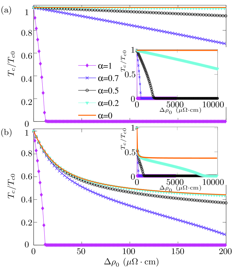
Figure 4: (Color online) $T_{c}/T_{c0}$ vs. $\Delta\rho_{0}$ for various values of the inter- to intraband scattering ratio $\alpha\equiv u/v$ with $v=1.25\mathrm{\;eV\,\mathcal{V}_{c}}$. (a) for isotropic $s\pm$ wave paring and (b) for an anisotropic (nodal) gap with anisotropy parameter $r=1.3$.

In this appendix we give some details of how our results change when taking values for the impurity parameters and pair potential parameters different from those used in the main text, so that the reader may judge how robust our conclusions are.

So far, we have focused on the parent compound BaFe₂As₂ and chosen values for the Fermi velocities and densities of states at the Fermi level that are compatible with both density functional theory (DFT) calculations Johnston10 and angle-resolved photoemission spectroscopy (ARPES) measurements.Evtushinsky09 ; Ding11 We assume a density of states on each Fermi surface sheet of $N_{a}=3.6$ and $N_{b}=2.7/\mathcal{V}_{c}$/eV/spin ($\mathcal{V}_{c}$ is the unit cell volume), for the “effective” hole and electron pockets, respectively, that approximately describes the imbalance in the densities of states that also has been seen with ARPES,Evtushinsky09 ; Ding11 ; Brouet09 and is consistent with the density of states of Ba122 arising from Fe $d$-orbitals according to DFT calculationsJohnston10 with an effective-mass renormalization of $z=3$. We take the root-mean-square Fermi velocities as $v_{\text{F},a}=2/3\times 10^{5}$ m/s and $v_{\text{F},b}=10^{5}$ m/s from Ref. Mishra11, , Table I, $v_{\text{F},\perp}$, and renormalize them by the same factor of $z=3$ to approximately match the velocities found in ARPES experiments.Evtushinsky09 ; Ding11 ; Brouet09 In the transport calculation, the component of the Fermi velocities in the direction of the current is taken to be $\langle v_{\text{F}\alpha,x}^{2}\rangle=1/2\,v_{\text{F}\alpha}^{2}$ due to the quasi-cylindrical Fermi surface. The pairing potentials chosen for the main text are $V_{aa}=V_{bb}=0.05$ and $V_{ab}=V_{ba}=-0.04$.

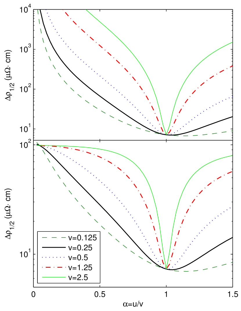
Figure 5: (Color online) The resistivity at half suppression $\Delta\rho_{1/2}$ as a function of the ratio $\alpha=u/v$ for various intraband impurity potentials $v$ (measured in $\text{eV}\,\mathcal{V}_{c}$); the other parameters are taken as in the main article for the isotropic $s_{\pm}$ wave pairing (top) and for an anisotropic (nodal) gap (bottom).

However, there are still two parameters unfixed, namely, the pairing potential $V_{\alpha\beta}$ and the impurity potential $v$ for scattering within bands (a full discussion of the variation of the inter- to intraband potential ratio $\alpha=u/v$ is included in Sec. V). Although the effective pairing potential $V_{\alpha\beta}$ and average coupling constant $\langle\lambda\rangle=\frac{1}{N_{a}+N_{b}}\sum_{\alpha,\beta\in\{a,b\}}N_{\alpha}V_{\alpha\beta}N_{\beta}$ as defined in Ref. Efremov11, for our weak-coupling model, as well as the impurity scattering potentials $u$ and $v$, are not known in experiments, our conclusions are consistent with different parameters within a reasonable range. If we increase $v$ to $v=1.25\mathrm{\;eV\,\mathcal{V}_{c}}$ keeping all other parameters identical to those of Fig. 2 of the main text, the $T_{c}$ suppression significantly slows, as seen in Fig. 4, with the exception of the value $\alpha=1$, which plays a special role in the theory of two-band $s_{\pm}$ superconductivity, as can be easily checked analytically. While in Ref. Kontani10, it was argued that the interband scattering potential $u$ should be generically large for any chemical substituent, there is no reason to expect $\alpha=1$ to hold exactly, and therefore we see that large critical resisitvities $\Delta\rho_{0}^{c}$ are even more likely to be found for stronger impurities (the unitarity limit $v\rightarrow\infty$ with fixed $\alpha$ is pathological in this modelEfremov11 and we have not considered it here). The special role of the value $\alpha=1$ can be illustrated by plotting the resistivity $\Delta\rho_{1/2}$ at which the critical temperature is suppressed by half, $T_{c}=0.5T_{c0}$, as shown in Fig. 5, which may be compared with experiments. Note that $\alpha\simeq 1$ yields the fastest $T_{c}$ suppression independent of the impurity potential in the physical regime $v\gtrsim u$.

Finally, we also mention the effect of choosing other pairing potentials $V_{\alpha\beta}$ that lead to different values of $\langle\lambda\rangle$. As explained in Ref. Efremov11, , for isotropic $s_{\pm}$ paring, when $T_{c}$ is plotted vs. the effective interband scattering rate, it follows three different universal curves according to whether $\langle\lambda\rangle$ is greater than, equal to, or less than 0. We have used a value $\langle\lambda\rangle=0.037\approx 0$ in our investigations. We have examined other parameter sets with negative $\langle\lambda\rangle$, and found no essential difference in $T_{c}$ when plotted against the residual resistivity $\Delta\rho_{0}$, which of course depends on both intra- and interband scattering.

References

- (1)
- (2)
- (3) P. J. Hirschfeld, M. M. Korshunov, and I. I. Mazin, Rep. Prog. Phys. 74, 124508 (2011).
- (4) A. Chubukov, Annu. Rev. Condens. Matter Phys. 3, 57 (2012).
- (5) I. I. Mazin, D. J. Singh, M. D. Johannes, and M. H. Du, Phys. Rev. Lett. 101, 057003 (2008).
- (6) H. Kontani and S. Onari, Phys. Rev. Lett. 104, 157001 (2010).
- (7) M. D. Lumsden, et al., Phys. Rev. Lett. 102, 107005 (2009).
- (8) A. D. Christianson, et al., Phys. Rev. Lett. 103, 087002 (2009).
- (9) D. S. Inosov, et al., Nat. Phys. 6, 178 (2010).
- (10) J. T. Park, et al., Phys. Rev. B 82, 134503 (2010).
- (11) D. N. Argyriou, et al., Phys. Rev. B 81, 220503 (2010).
- (12) J.-P. Castellan, et al., Phys. Rev. Lett. 107, 177003 (2011).
- (13) T. Hanaguri, S. Niitaka, K. Kuroki, and H. Takagi, Science 328, 474 (2010).
- (14) C.-T. Chen, et al., Nat. Phys. 6, 260 (2010).
- (15) Y. Senga and H. Kontani, J. Phys. Soc. Jpn. 77, 113710 (2008).
- (16) Y. Senga and H. Kontani, New J. Phys. 11, 035005 (2009).
- (17) S. Onari and H. Kontani, Phys. Rev. Lett. 103, 177001 (2009).
- (18) J. Li, et al., Phys. Rev. B 85, 214509 (2012).
- (19) K. Kirshenbaum, et al., Phys. Rev. B 86, 140505 (2012).
- (20) Y. Li, et al., New J. Phys. 12, 083008 (2010).
- (21) Y. Nakajima, et al., Phys. Rev. B 82, 220504 (2010).
- (22) M. Tropeano, et al., Phys. Rev. B 81, 184504 (2010).
- (23) A. Abrikosov and L. Gor’kov, Sov. Phys. JETP 12, 1243 (1961).
- (24) G. Preosti and P. Muzikar, Phys. Rev. B 54, 3489 (1996).
- (25) A. A. Golubov and I. I. Mazin, Phys. Rev. B 55, 15146 (1997).
- (26) A. Golubov and I. Mazin, Physica C 243, 153 (1995).
- (27) D. Parker, et al., Phys. Rev. B 78, 134524 (2008).
- (28) A. V. Chubukov, D. V. Efremov, and I. Eremin, Phys. Rev. B 78, 134512 (2008).
- (29) Y. Bang, H.-Y. Choi, and H. Won, Phys. Rev. B 79, 054529 (2009).
- (30) V. Mishra, et al., Phys. Rev. B 79, 094512 (2009).
- (31) A. A. Golubov, et al., Phys. Rev. B 66, 054524 (2002).
- (32) V. G. Kogan, C. Martin, and R. Prozorov, Phys. Rev. B 80, 014507 (2009).
- (33) M. L. Kulić and O. V. Dolgov, Phys. Rev. B 60, 13062 (1999).
- (34) Y. Ohashi, Physica C 412, 41 (2004).
- (35) D. V. Efremov, et al., Phys. Rev. B 84, 180512 (2011).
- (36) A. F. Kemper, C. Cao, P. J. Hirschfeld, and H.-P. Cheng, Phys. Rev. B 80, 104511 (2009).
- (37) A. F. Kemper, C. Cao, P. J. Hirschfeld, and H.-P. Cheng, Phys. Rev. B 81, 229902 (2010).
- (38) K. Nakamura, R. Arita, and H. Ikeda, Phys. Rev. B 83, 144512 (2011).
- (39) S. Graser, P. J. Hirschfeld, L.-Y. Zhu, and T. Dahm, Phys. Rev. B 76, 054516 (2007).
- (40) L. Zhu, P. J. Hirschfeld, and D. J. Scalapino, Phys. Rev. B 70, 214503 (2004).
- (41) F. Gross, et al., Z. Phys. B 64, 175 (1986).
- (42) L. Gor’kov and P. Kalugin, JETP Lett. 41, 208 (1985).
- (43) K. Ueda and T. Rice, Theory of Heavy Fermions and Valence Fluctuations (Springer-Verlag, Berlin, 1985).
- (44) P. J. Hirschfeld and N. Goldenfeld, Phys. Rev. B 48, 4219 (1993).
- (45) L. S. Borkowski and P. J. Hirschfeld, Phys. Rev. B 49, 15404 (1994).
- (46) A. V. Balatsky, I. Vekhter, and J.-X. Zhu, Rev. Mod. Phys. 78, 373 (2006).
- (47) D. C. Johnston, Adv. Phys. 59, 803 (2010).
- (48) D. V. Evtushinsky, et al., New Journal of Physics 11, 055069 (2009).
- (49) H. Ding, et al., Journal of Physics: Condensed Matter 23, 135701 (2011).
- (50) V. Brouet, et al., Phys. Rev. B 80, 165115 (2009).
- (51) V. Mishra, S. Graser, and P. J. Hirschfeld, Phys. Rev. B 84, 014524 (2011).