Boson features in STM spectra of cuprate superconductors: Weak-coupling phenomenology

Abstract

We derive the shape of the high-energy features due to a weakly coupled boson in cuprate superconductors, as seen experimentally in $Bi_{2}Sr_{2}Ca_{1}Cu_{2}O_{8+x}$ (BSCCO) by Lee et al [Nature 442, 546 (2006)]. A simplified model is used of $d$-wave Bogoliubov quasiparticles coupled to Einstein oscillators with a momentum independent electron-boson coupling and an analytic fitting form is derived, which allows us (a) to extract the boson mode’s frequency, and b) to estimate the electron-boson coupling strength. We further calculate the maximum possible superconducting gap due to an Einstein oscillator with the extracted electron-boson coupling strength which is found to be less than 0.2 times of the observed gap indicating at the observed boson’s non-dominant role in the superconductivity’s mechanism. The extracted momentum-independent electron-boson coupling parameter (that we show a posteriori to indeed be in the weak-coupling regime) is then to be interpreted as an (band-structure detail dependent weighted) average over the Brillouin Zone of the actual momentum-dependent electron-boson coupling in BSCCO.

I Introduction

Scanning tunneling microscopy (STM), applied to the superconducting cuprate Bi₂Sr₂Ca₁Cu₂O_8+x (BSCCO 2212) Jinho , found a feature in the density of states (DOS) at an energy well above the energy scale of the so-called coherence peak energy (Fig. 1), and attributed it to an electron-boson coupling. In conventional (s-wave) superconductors (e.g. Hg, Pb, Al), such features due to electron-phonon coupling were known in tunneling spectra from superconductor-insulator-normal metal junctions McMillan ; SC-tunnel-reviews . The phonon frequencies inferred from the tunneling feature agreed with the phonon density of states inferred from neutron scattering; furthermore, the phonon-mediated superconducting $T_{c}$ and gap were correctly predicted McMillan from the tunneling using the Eliashberg formalism Eliashberg . In the case of cuprates, the mechanism for superconductivity is not established, and there are divergent opinions whether the mode observed by Lee et al contributes to the pairing Jinho ; Carbotte2 ; Balatsky-localpairing ; Johnston2 .

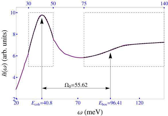
Figure 1: A typical measured STM spectrum in BSCCO (proportional to DOS  $n({\omega})$) as a function of energy $E$; the data was provided by Jacob Alldredge. Energies of the “coherence peak” $E_{\rm coh}$ and boson feature $E_{\rm bos}$ are indicated. Boxes show energy windows used to fit the analytic form (see Fig. 3, below.)

In BSCCO, the pairing strength is highly inhomogeneous at the nanoscale McElroy ; inhomogeneity-refs:Pan ; inhomogeneity-refs:Cren ; inhomogeneity-refs:Howald ; inhomogeneity-refs:Lang ; inhomogeneity-refs:Fang , as inferred from the spatial fluctuations of the energy $E_{\rm coh}$ of the “coherence peak” in STM spectra (Figure 1). Lee et al discovered that the boson feature’s energy $E_{\rm bos}$ “floats” with the same inhomogeneity as $E_{\rm coh}$, namely $E_{\rm bos}=E_{\rm coh}+\hbar\Omega_{0}$ with a (spatially uniform) boson frequency $\Omega_{0}$. To infer $E_{\rm bos}$, they identified it as the inflection point in DOS $n({\omega})$ before the feature. In this paper, we improve on this recipe by deriving an analytic formula for the boson feature, starting from the simplest phenomenological model of a cuprate and using basic RPA calculations. Our focus here is the energy dependence rather than the spatial modulations  Zhu1 ; Zhu2 of this feature. Prior calculations Johnston ; de_Castro addressed the same question of extracting $\Omega_{0}$ from from the shape of the DOS  of BSCCO. Ref. Johnston, uses more elaborate (Eliashberg) calculation, but in an entirely numerical framework, making the physical interpretation indirect and the method computationally bulky to use for fitting vast number of spectra that STM affords us with. However, Ref. Johnston, and related Ref. Johnston2, have extensively discussed the material details about the electron-boson coupling and related form factors, that we intentionally avoid in favour of simplicity.

We first ask just what point in the feature is to be identified as $E_{\rm bos}$: our recipe implies a value for $\hbar\Omega_{0}$ in basic agreement with the analysis in Ref. Jinho, . Secondly, we ask how can one can extract the electron-boson coupling strength; our results indicate it is indeed small enough that our weak-coupling approximation is justified, and furthermore this coupling alone is unlikely to explain the magnitude of the observed superconducting gap.

II Weak-coupling Model

We begin by setting up the simplest possible model, taking the electron-boson coupling as a small perturbation to an already superconducting fermion dispersion of the standard mean-field form (as in Ref. Zhu1, ; de_Castro, ; Eschrig-Norman, ; Berthod, ), and then setting up the DOS  calculation within the RPA approximation. Our analysis is agnostic as to the boson’s nature, which is sometimes argued to be magnetic Carbotte2 , but usually considered to be an oxygen vibration, on account of the O¹⁸ isotope effect Jinho .

Our bare fermion Hamiltonian has the usual mean-field form

$${\cal H}=\sum_{{\bf{k}},\sigma}\epsilon({\bf{k}})c^{\dagger}_{{\bf{k}},\sigma}c_{{\bf{k}},\sigma}+\Delta({\bf{k}})c_{{\bf{k}},\sigma}c_{-{\bf{k}},-\sigma}+h.c.$$ (1)

where $\epsilon({\bf{k}})$ is the normal-state band dispersion, for which (in all numerical calculations in this paper) we adopt a six-parameter tight-binding fit to ARPES data on BSCCO based on Ref. Norman, . The quasiparticle dispersion is then $E({\bf{k}})=\sqrt{\epsilon({\bf{k}})^{2}+\Delta({\bf{k}})^{2}}$, where we will assume $d$-wave pairing with

$$\Delta({\bf{k}})\equiv\frac{\Delta_{0}}{2}\left[\cos(k_{x})-\cos(k_{y})\right].$$ (2)

We (plausibly) approximate the bosonic mode as a dispersionless (Einstein) oscillator at frequency $\Omega_{0}$, and assume an electron-phonon coupling

$${\cal H}_{\text{e-ph}}=\frac{1}{\sqrt{N}}\sum_{{\bf{k}},{\bf{q}},\sigma}g({\bf{q}})c^{\dagger}_{{\bf{k}}+{\bf{q}},\sigma}c_{{\bf{k}},\sigma}(b_{-{\bf{q}}}+b^{\dagger}_{\bf{q}})$$ (3)

where $b^{\dagger}_{\bf{q}}$ and $b_{\bf{q}}$ are the bosonic creation and annihilation operators, and $N$ is the number of lattice sites. For simplicity we work through the case $g({\bf{q}})\equiv g$; after completing that, we will revisit the more general case with a momentum-dependent $g({\bf{q}})$.

Our object, the DOS, is defined as the trace of the electron term in the Green’s function:

$$n({\omega})\equiv-\frac{1}{\pi}{{\rm Tr}_{\bf{k}}}\;{\rm Im}\,G_{11}({\bf{k}},{\omega}),$$ (4)

where ${{\rm Tr}_{\bf{k}}}\equiv a^{2}\int_{\rm B.Z.}d^{2}{\bf{k}}/(2\pi)^{2}$, and the integral is over the Brillouin zone. In the $2\times 2$ Nambu formalism, the bare Green’s function is given by

$${{\underline{G}}^{0}}({\bf{k}};{\omega})^{-1}=\left(\begin{array}[]{lr}{\omega}-\epsilon({\bf{k}})&\Delta({\bf{k}})\\ \Delta({\bf{k}})^{*}&{\omega}+\epsilon({\bf{k}})\\ \end{array}\right).$$ (5)

We shall henceforth use Pauli matrices ${\underline{\tau}}_{i}$, and adopt the gauge in which $\Delta_{0}$ is real: thus ${{\underline{G}}^{0}}=[E{\underline{\mathbb{I}}}+\epsilon({\bf{k}}){\underline{\tau}}_{3}+\Delta({\bf{k}}){\underline{\tau}}_{1}]/[{\omega}^{2}-E({\bf{k}})^{2})]$. The boson propagator has the form

$$D({\bf{q}};\Omega)=\frac{1}{2}\left(\frac{1}{\Omega-\Omega_{0}}-\frac{1}{\Omega+\Omega_{0}}\right)\equiv D(\Omega).$$ (6)

III Self-Energy and density of states due to the boson

The boson feature enters the DOS  via the dressed Green’s function, in the RPA approximation,

$${\underline{G}}({\bf{k}},{\omega})^{-1}={{\underline{G}}^{0}}({\bf{k}},{\omega})^{-1}-{\underline{\Sigma}}({\bf{k}},{\omega}).$$ (7)

Because $\Omega_{0}$ and $D(\Omega)$ were momentum-independent, so is the electronic self energy, reducing (at lowest order in $g$) to ${\underline{\Sigma}}({\bf{k}},{\omega})\equiv{\underline{\Sigma}}({\omega})$, where

$${\underline{\Sigma}}({\omega})=g^{2}\int\frac{d\Omega}{2\pi}D(\Omega)\;{{\rm Tr}_{\bf{q}}}\{{\underline{\tau}}_{3}\;{{\underline{G}}^{0}}({\bf{k}}-{\bf{q}};{\omega}-\Omega){\underline{\tau}}_{3}\}$$ (8)

After a contour evaluation of the $\Omega$ integral Eq. (8) reduces to

$${\underline{\Sigma}}({\omega}) = \frac{g^{2}}{2}{{\rm Tr}_{\bf{k}}}\Bigg{\{}\frac{({\omega}+\Omega_{0}){\underline{\mathbb{I}}}+\epsilon({\bf{k}}){\underline{\tau}}_{3}-\Delta({\bf{k}}){\underline{\tau}}_{1}}{({\omega}+\Omega_{0})^{2}-E({\bf{k}})^{2}}$$ (9)

$$+\frac{\Omega_{0}({\underline{\mathbb{I}}}+\frac{\epsilon({\bf{k}})}{E({\bf{k}})}{\underline{\tau}}_{3}-\frac{\Delta({\bf{k}})}{E({\bf{k}})}{\underline{\tau}}_{1})}{[{\omega}-E({\bf{k}})]^{2}-\Omega_{0}^{2}}.\Bigg{\}}$$

The off-diagonal (${\underline{\tau}}_{1}$) terms in Eq. (9) vanish, $\Sigma_{12}=\Sigma_{21}\equiv 0$, since $\Delta_{{\bf{k}}}$ has $d$-wave symmetry (reverses sign under 90^∘ rotations).

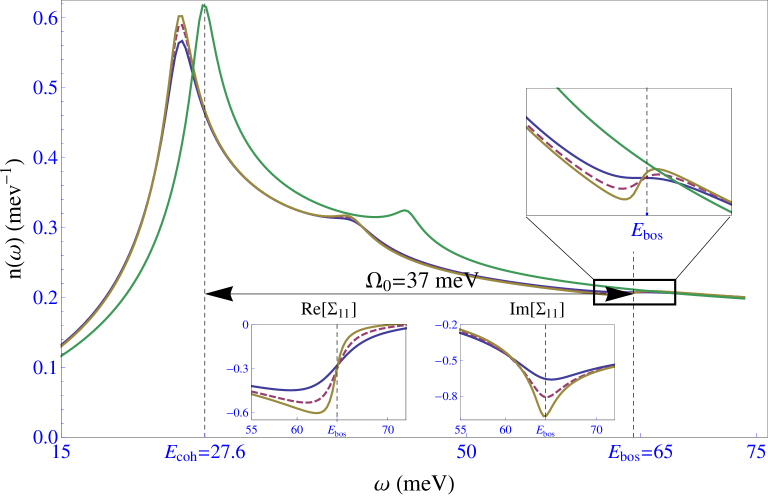
Figure 2: [COLOR ONLINE] Numerically computed DOS  as a function of energy. The standard six-parameter dispersion for BSCCO was used Norman ; we chose the pairing amplitude to be $\Delta_{0}=0.2|t_{1}|\approx 29.6$ meV, the boson energy to be $\hbar\Omega_{0}=0.25|t_{1}|\approx 37$ meV and electron-boson coupling to be $g=\sqrt{0.1}|t_{1}|\approx 47$ meV, where $t_{1}$ is the nearest-neighbor hopping. Three different choices of damping are shown: from sharpest to flattest, $\eta=0.005$, $0.01$ and $0.02$ (in units of $t_{1}$). Lower inset shows real and imaginary parts of the electron self-energy function. This has singularities at $E_{\rm bos}$ rounded by the damping.

We write $n({\omega})=n_{0}({\omega})+\delta n({\omega})$, where $n_{0}({\omega})$ is tbe basic DOS  in the absence of the boson coupling [derived from (5)] and has the well-known “coherence peaks” centered at energy values $\pm E_{\rm coh}$ close to $\pm\Delta_{0}$; $\delta n({\omega})$ contains contributions of order $g^{2}$, in particular the boson feature. Writing the Taylor expansion of (7), we extract the terms in $G_{11}$ linear in ${\underline{\Sigma}}$ and thus

$$\delta n({\omega}) = -\frac{1}{\pi}{\rm Im}{{\rm Tr}_{\bf{k}}}\left\{\frac{[{\omega}+\epsilon({\bf{k}})]^{2}\Sigma_{11}({\omega})+|\Delta({\bf{k}})|^{2}\Sigma_{22}({\omega})}{[{\omega}^{2}-E({\bf{k}})^{2}]^{2}}\right\}$$ (10)

$$\equiv \frac{1}{\pi}{\rm Im}\left\{I_{1}({\omega})\Sigma_{11}({\omega})+I_{2}({\omega})\Sigma_{22}({\omega})\right\}.$$

This is the first version of our result, suitable for numerical fits Jacob-new , but requiring integrations over the zone at each interation [for the key formulas  (9) and  (10). Note that in numerical calculations, we replace $\omega\to\omega+i\eta$ in (5), where $i\eta$ represents the physical quasiparticle damping (from all sources except our boson mode), a parameter found essential for fitting the “coherence peaks” in the DOS Jacob . (It is easy to replace this energy-independent damping by $\eta({\omega})$, as used in Ref. Jacob . Fig. 2 shows a representative numerical calculation of the self-energy function (inset) and the resulting DOS. We see a dip-hump shape, in agreement with experiment; $E_{\rm bos}$ falls between the dip and the hump similar to the assumption of Ref. Jinho .

IV Asymptotic Form near $E_{\rm bos}=E_{\rm coh}+\Omega_{0}$

We now extend our results to an approximate analytic formula, for the boson feature’s shape, by treating not only the electron-boson coupling $g$, but also the damping $\eta$ as a small parameter: in the limit $\eta\to 0$ the feature is a singularity centered at $E_{\rm bos}\equiv E_{\rm coh}+\Omega_{0}$.

First recollect the origin of the familiar “coherence peak” in the basic DOS  $n_{0}({\omega})$: it is a van Hove singularity due to the saddle points at ${\bf{k}}=({k_{s}},\pi)$ and equivalent momenta where the Fermi surface crosses the zone boundary. The pertinent pole in ${\underline{G}}_{0}$ is $\frac{1}{2}[{\omega}-E({\bf{k}})]^{-1}{\underline{\mathbb{I}}}$; there is no contribution from ${\underline{\tau}}_{3}$ due to the factor $\epsilon({\bf{k}})$ which vanishes on the Fermi surface. It is well known that ${{\rm Tr}_{\bf{k}}}[{\omega}-E({\bf{k}})]$ at a saddle gives a logarithmic singularity, so we find a singular part

$$n_{0}^{\rm sing}({\omega})=-\frac{a^{2}{m^{*}}}{\pi^{2}}{\rm Re}f({\omega}-E_{\rm coh}+i\eta_{\rm coh})$$ (11)

with

$$f(z)\equiv\ln({m^{*}}z/4K_{x}K_{y}).$$ (12)

Here $E({\bf{k}})\approx E_{\rm coh}+(k_{x}-{k_{s}})^{2}/2{m_{x}}-(k_{y}-\pi/a)^{2}/2{m_{y}}$ near the saddle, ${m^{*}}\equiv\sqrt{{m_{x}}{m_{y}}}$, and $K_{x}$, $K_{y}$ are cut-offs, representing the range of $(k_{x},k_{y})$ within which this expansion is valid. For our parameters, $1/{{m^{*}}}=94.07$meV $a^{2}$, and we take $K_{x}=0.5a^{-1}$ and $K_{y}=0.06a^{-1}$ for later numerical calculations.

The self-energy ${\underline{\Sigma}}(E)$ has a singularity due to the same saddle point, with the pole of form $(\frac{1}{2})^{2}g^{2}{\underline{\mathbb{I}}}[{\omega}-E({\bf{k}})-\Omega_{0}]^{-1}$, coming from the second big term in (9). Clearly, integrating over ${\bf{k}}$ gives the same logarithmic divergence, with its argument shifted by $\Omega_{0}$. Thus,

$${\underline{\Sigma}}({\omega}+i\eta)=\text{regular terms}+\frac{ig^{2}a^{2}}{2\pi}{m^{*}}f({\omega}-E_{\rm bos}+i\eta){\underline{\mathbb{I}}}$$ (13)

with $f(z)$ from (12). This behavior is confirmed by the inset of Fig. 2.

The ${\underline{\mathbb{I}}}$ dependence in (13) signifies that $\Sigma_{11}\approx\Sigma_{22}$ at the singularity. Thus (10) simplifies to

$$\delta n^{\rm sing}({\omega})=\frac{1}{\pi}{\rm Im}[\Sigma_{11}({\omega})I(E_{\rm bos}+i\eta)],$$ (14)

with $I({\omega})\equiv[I_{1}({\omega})+I_{2}({\omega})]/2$ (see Eq. 10).

Thus our key asymptotic result is that $\delta n({\omega})$ has a logarithmic singularity at $E_{\rm bos}$, rounded by the finite damping $\eta$. The result is a linear combination of a rounded step and a cut-off log divergence, with the exact shape (and the location of $E_{\rm bos}$ within it) depending on the phase angle in $I({\omega})\equiv|I({\omega})|e^{i\phi_{I}}$, which depends on the band structure [cf. Eq. (14)].

For energies around the boson feature (e.g. ${\omega}\approx 115$ meV), the rough dependence on damping is $I({\omega}+i\eta)=1.5\times 10^{-5}(\eta-15)+0.7\times 10^{-3}i$. Thus, the shape of $\delta n({\omega})$ is a (comparable) combination of a rounded upwards step from ${\rm Re}\Sigma_{11}$ and a rounded logarithmic hump from ${\rm Im}\Sigma_{11}$ leading to location of the boson mode frequency ${\omega}$ before the hump (as seen in numerics cf. Fig. 2).

We can attach physical interpretationsSumi-thesis to the real and imaginary parts of $\Sigma_{22}({\omega})$. The imaginary part represents an inelastic event in which a real boson excitation is created; the real part represents the quasiparticle being dressed by virtual bosons.

Since the predicted feature includes a “step up”, we are in agreement with the recipe of Lee et al which placed $E_{\rm bos}$ at the inflection point before the hump of the boson feature, motivated by previous work on molecular vibrational features in electron tunneling Jaklevic ; Stipe . Refs. Johnston, , de_Castro, and Pasupathy, located $E_{\rm bos}$ even lower, at the minimum of the dip in the dip-hump feature. As mentioned before, we also place $E_{\rm bos}$ before the hump but more specifically in between the hump and its preceding inflection point.

We can attempt to compare our self-energy functions with those of Ref. Johnston [(Figure 3(c)], computed numerically from Eliashberg theory. ${\rm Re}\Sigma_{ii}({\omega})$ is proportional to their ${\rm Im}Z(\omega)$ which indeed resembles a (positive) log divergence, while ${\rm Im}\Sigma_{ii}\propto 1-Z(\omega)$ shows a rounded up step.

V Fitting Scheme for the Experimental Boson Feature

In this section, we translate our asymptotic forms to a simplified fitting scheme for our weak-coupling model and, by applying it to the experimental spectrum in Fig. 1, extract the $E_{\rm bos}$ and also obtaining the electron-boson coupling $g$ from the boson feature’s amplitude E>0 . We consider the experimental signal to be in arbitrary units so we write it $\tilde{n}({\omega})=\beta_{\rm cal}n({\omega})$, where the coefficient $\beta_{\rm cal}$ includes unknown factors such as the STM tip set-point. As the dispersion $\epsilon({\bf{k}})$ is already known from ARPES Norman , the “coherence peak” is sufficiently constrained that we can calibrate $\beta_{\rm cal}$ from it. We read off $E_{\rm coh}=40.8$ meV from the peak position in Fig. 1. From this, using $E_{\rm coh}=E({\bf{k}}_{\rm saddle})$, we infer $\Delta_{0}=44.23\text{meV}$.

The saddle point of the quasiparticle dispersion at ${\bf{k}}_{\rm saddle}$ contributes a logarithmic singularity to the DOS  at the “coherence peak”:

$$n_{0}({\omega})=n^{\rm reg}({\omega})+n_{0}^{\rm sing}({\omega})$$ (15)

where $n_{0}^{\rm sing}({\omega})$ is given by (11), and we adopt the simplest usable form $n^{\rm reg}({\omega})=a_{\rm coh}{\omega}+b_{\rm coh}$ for the regular part, which is due mainly to $n_{0}({\omega})$.

$\Delta_{0}$	44.23 meV	$\Omega_{0}$	56(1) meV
$\beta_{\rm cal}$	3.2(4)$\times$104 arb. units meV-1	g	36(16) meV
$\eta_{\rm coh}$	10.7(9) meV	$\eta_{\rm bos}$	11(2) meV
$a_{\rm coh}$	3.1(2) $\times$ 10-2 meV-2	$a_{\rm bos}$	0.40(35) $\times$ 10-2 meV-2
$b_{\rm coh}$	8.1(7) meV-1	$b_{\rm bos}$	6.9(5) meV-1

Table 1: Fit parameters for the “coherence peak” using Eq. (15) (left column) and for the boson feature using Eq. (16) (right column). The error-bars on the fit parameters were estimated by determining the parameter range where $\chi^{2}\leq 2*\chi^{2}_{min}$, where $\chi^{2}=\sum_{i}(y_{i}-f(x_{i}))^{2}$, $i$ is the (energy) index for data-points, $y_{i}$ and $f(x_{i})$ are the experimental datum and the value of fitting function respectively at the $i$-th data point.

Table 1 gives the results of the calibration fit to the data in Fig. 1, using energies in (30 meV, 50 meV). As Fig. 3 (left panel) shows, the fitting is good in this window. This fit gives a quasiparticle broadening $\eta_{\rm coh}\approx 10$ meV (assumed to be constant over the Brillouin zone and the energy window $30-50meV$), uncomfortably large in that $\eta_{\rm coh}/E_{\rm coh}\approx 1/4$. We do not know why this exceeds the result $\eta(E_{\rm coh}\approx 40\text{meV})\approx 1$ meV. fitted by Ref. Jacob, assuming a broadening $\eta({\omega})\propto{\omega}$.

a)

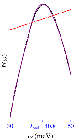
b)

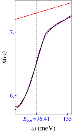
Figure 3: Fit of the experimental DOS  $n({\omega})$ to fitting forms, using the windows of energies marked in Fig. 1. (a) Fit of “coherence peak” to Eq. (15), using energies 30–50 meV. (b) Fit of boson feature to Eq. (16), using energies 80–140 meV.

Now we turn to the fit of the boson feature, using an energy window (80 meV, 140 meV) which contains the hump in Fig. 1, to the fitting form implicit in Eqs. (10) [for $I({\omega})$],  (13), and  (14):

$$n({\omega})=n_{\rm bos}^{\rm reg}({\omega})+\delta n^{\rm sing}({\omega}).$$ (16)

Here we take the simplest usable form for the regular part $n_{\rm bos}^{\rm reg}({\omega})=a_{\rm bos}{\omega}+b_{\rm bos}$, representing $n_{0}({\omega})$ plus regular contributions from ${\underline{\Sigma}}(E)$. Also from (14) we see

$$\delta n^{\rm sing}({\omega}) = \frac{2ig^{2}a^{2}{m^{*}}}{(2\pi)^{4}}\times$$ (17)

$$\times{\rm Im} \left[I({\omega}+i\eta_{\rm bos})\cdot f({\omega}-E_{\rm bos}+i\eta_{\rm bos})\right]$$

The fitted parameters are given in Table 1; the fit (Fig. 3) is fairly good in its energy window.

We note that, based on the data from which Fig. 1 is drawn, Ref. Jinho identified the bosonic mode energy as $52\pm 8$ meV, using the inflection point before the hump, so our result of $56\pm 1$ meV (fitting just one typical spectrum) is in agreement with them. The quasiparticle damping was $\eta_{\rm bos}\approx 11\text{meV}$. Thus $\eta({\bf{k}})/E({\bf{k}})\approx\eta_{\rm bos}/E_{\rm bos}\approx 0.11\ll 1$ in the $E_{\rm bos}$ fit window, verifying the criterion for the Bogoliubov quasiparticles to be well-defined.

A dimensionless measure of coupling strength is the the ratio of the logarithmic factors $f(z)$ in the boson feature [Eq. (16)] and coherence peak [Eq. (15)]:

$$\lambda_{\rm log}\equiv\frac{2g^{2}|I(E_{\rm bos}+i\eta_{\rm bos})|}{(2\pi)^{2}}\approx 0.057,$$ (18)

using the numerical value $|I(E_{\rm bos}+i\eta_{\rm bos})|=8.7\times 10^{-4}$ meV^-2, validating our weak-coupling assumption.

VI Momentum-dependent boson coupling and gap renormalization

What if the electron-boson coupling $g({\bf{q}})$ in (3) is not constant but depends on the electron momentum transfer ${\bf{q}}$? Firstly, it gives renormalizations of $\Delta({\bf{k}})$ due to $\Sigma_{12}$ which is no longer zero (see Eqs.(4) and (5)). To obtain an upper bound for the gap renormalization, we try the form for ${\bf{q}}$ dependence which leads to the maximal renormalization, namely $|g({\bf{q}})|^{2}=\tilde{g}^{2}[\frac{1}{2}(\cos q_{x}+\cos q_{y})]$, where we set $\tilde{g}$ to the fitted $g$ value from Table 1. We compute the gap renormalization using the obvious generalization of Eq. (8) to account for ${\bf{q}}$ dependence of electron-boson coupling in the off-diagonal components of Eq. 8 (See A.1 for details). We find that for all energies, the gap renormalization is less than 5 meV (See Fig. 4), which is small enough compared to $\Delta_{0}$ to justify our weak-coupling assumption, but not so small to categorically rule out some contribution by the boson to pairing.

For the boson feature, the overall structure of the calculation carries through but the self-energy ${\underline{\Sigma}}$ becomes momentum dependent. We find the same sort of DOS  feature, in which “$g^{2}$” is now interpreted as a certain weighted average of $|g({\bf{q}})|^{2}$ over the Brillouin zone – a lumped parameter in the spirit of the “$\alpha^{2}F(\omega)$” combination from the strong-coupling formalism McMillan . The singularity in the self energy still come from the saddle point in the dispersion of the $d$-wave BCS quasiparticles, leading to the same qualitative shape (smoothed step + logarithm) for the boson feature . See A.2 for details.

VII Conclusion and Discussion

We have shown how a weak-coupling point of view can be used to analyze the high-energy features in the STM data of BSCCO. The ideal analytic shape of the feature is a linear combination of a (rounded) logarithmic-kink and a (rounded) step edge [cf. Eq. (14)]. Our proposed fitting scheme allowed us to extract (1) the boson’s frequency $\Omega_{0}$ (2) an average electron-boson coupling $g$, and an estimate of the damping of the $d$-wave Bogoliubov quasiparticles. Our estimate $\Omega_{0}\approx 56$ meV is in agreement with previous estimates from STM data, which were not fully in agreement with ARPES data ARPES_1 ; ARPES_2 ; ARPES_3 ; ARPES_4 ; ARPES_5 , (ARPES results suggest $\Omega_{0}\approx 40$ meV.)

Our simplified simple functional form for the boson feature [Eq. (16)] facilitates the vast number of numerical fits required by the extreme spatial inhomogeneity of STM spectra in BSCCO McElroy ; inhomogeneity-refs:Pan ; inhomogeneity-refs:Cren ; inhomogeneity-refs:Howald ; inhomogeneity-refs:Lang ; inhomogeneity-refs:Fang ; Jacob . However, our theory did not address the spatial Fourier spectrum of the boson feature Jinho ; Zhu1 ; Zhu2 , which might distinguish the true functional form of $g({\bf{q}})$ and thus illuminate the nature of the bosonic mode.

Our approach was agnostic as to the pairing mechanism. If the fitted $g$ respects the weak-coupling assumption - as we found for a typical spectrum - it can be inferred that the boson producing the STM feature is not contributing significantly to the pairing; if the weak-coupling assumption were to be violated, we can only conclude that the boson perhaps plays a role in the main mechanism. To resolve that question, one must see if a strong-coupling Eliashberg calculation predicts a pairing amplitude $\Delta_{0}$ comparable to the observed value.

Appendix A Effects of Momentum Dependent Electron-Phonon Coupling

We quickly recall the basic formula for the weak-coupling self-energy where we have now an explicitly momentum dependent electron boson coupling $g({\bf{q}})$ and self-energy ${\underline{\Sigma}}({\bf{k}},{\omega})$

$${\underline{\Sigma}}({\bf{k}};{\omega}) = \int_{\rm B.Z.}\frac{d^{2}{\bf{q}}}{(2\pi)^{2}}\frac{g({\bf{q}})^{2}}{2}\Bigg{\{}\frac{({\omega}+\Omega_{0}){\underline{\mathbb{I}}}+\epsilon({\bf{k}}-{\bf{q}}){\underline{\tau}}_{3}-\Delta({\bf{k}}-{\bf{q}}){\underline{\tau}}_{1}}{({\omega}+\Omega_{0})^{2}-E({\bf{k}}-{\bf{q}})^{2}}+\frac{\Omega_{0}({\underline{\mathbb{I}}}+\frac{\epsilon({\bf{k}}-{\bf{q}})}{E({\bf{k}}-{\bf{q}})}{\underline{\tau}}_{3}-\frac{\Delta({\bf{k}}-{\bf{q}})}{E({\bf{k}}-{\bf{q}})}{\underline{\tau}}_{1})}{[{\omega}-E({\bf{k}}-{\bf{q}})]^{2}-\Omega_{0}^{2}}.\Bigg{\}}$$ (19)

As was mentioned in the main text, the two effects of the momentum dependent electron-boson coupling $g(\mathbf{q})$ are 1) renormalization of the bare d-wave gap $\Delta(\mathbf{k})$, and 2) the self-energy will no longer momentum independent (as in the main text).

A.1 Renormalization of the bare d-wave gap

Consistency of the weak-coupling assumption requires expectedly that the renormalization of the bare d-wave gap should be at most a non-appreciable fraction of the bare gap. This is a different consistency check than done in the main text using $\lambda_{log}$. $\lambda_{log}$ instead measures the smallness of the diagonal components of the self-energy ${\underline{\Sigma}}_{11}$ and ${\underline{\Sigma}}_{22}$ with respect to that of the diagonal components of the bare (inverse) Green’s function. To estimate an upper bound for the gap renormalization, we tried the form for ${\bf{q}}$ dependence which leads to the maximal renormalization, namely $g({\bf{q}})^{2}=\tilde{g}^{2}[\frac{1}{2}(\cos q_{x}+\cos q_{y})]$, where we set $\tilde{g}$ to $50$ meV which is the fitted $g$ plus one error-bar on it. We computed the gap renormalization using Eq. (9) which is

$${\underline{\Sigma}}_{12}({\omega}) = \int_{\rm B.Z.}\frac{d^{2}{\bf{q}}}{(2\pi)^{2}}\frac{g({\bf{q}})^{2}}{2}\Bigg{\{}\frac{-\Delta({\bf{k}}-{\bf{q}})}{({\omega}+\Omega_{0})^{2}-E({\bf{k}}-{\bf{q}})^{2}}$$ (20)

$$+\frac{\Omega_{0}(-\frac{\Delta({\bf{k}}-{\bf{q}})}{E({\bf{k}}-{\bf{q}})})}{[{\omega}-E({\bf{k}}-{\bf{q}})]^{2}-\Omega_{0}^{2}}.\Bigg{\}}$$

to account for ${\bf{q}}$ dependence of electron-boson coupling in (the off-diagonal components of) Eq. 9. We find that for all energies, the gap renormalization is less than 5 meV as shown in Fig. 4. This is small enough compared to $\Delta_{0}\approx 40$ meV to justify our weak-coupling assumption, but not so small to categorically rule out some contribution by the boson to pairing. A small contribution of the observed boson to the superconductivity that is dominantly established by the as-yet-unknown mechanism is not unrealistic phenomenologically.

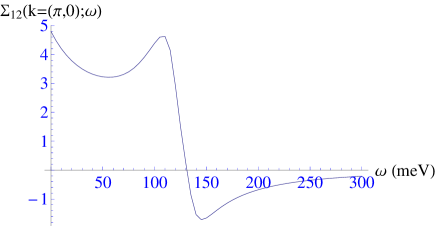
Figure 4: In this figure is shown the maximal gap renormalization due to a momentum dependent electron boson coupling for our chosen band-structure and extracted boson frequency and electron boson coupling strength. We adopt the six-parameter fit from M. R. Norman et al, Phys. Rev. B 52, 615 (1995): hopping amplitudes to successive neighbors of $t_{1}=-147.9$ meV, $t_{2}=40.9$ meV, $t_{3}=-13.0$ meV, $t_{4}=-14.0$ meV and $t_{5}=12.8$ meV, plus a chemical potential $\mu=130.5$ meV as in main text. See Table I of the main text for the values of the fitted parameters. We have plotted for the particular momentum ($\pi$,0). Similar magnitudes are obtained for other momenta.

A.2 Effect on the boson feature

Firstly we recall that for the momentum independent electron boson coupling, the off-diagonal part of the self-energy is identically zero as mentioned in the main text. According to our analysis for the diagonal parts, the singular contributions are equal for $\Sigma_{11}$ and $\Sigma_{22}$. They are of the form $(ig^{2}a^{2}m^{*}/2\pi)\log[({\omega}-E_{coh}-\Omega_{0})m^{*}/K_{x}K_{y}]$ + regular terms. Here $E({\bf{k}})\approx E_{\rm coh}+(k_{x}-{k_{s}})^{2}/2{m_{x}}-(k_{y}-\pi/a)^{2}/2{m_{y}}$ near its saddle points (here in this expression assumed to be ${\bf{K}}_{*}=({k_{s}},0)$; there are four such saddle points), ${m^{*}}\equiv\sqrt{{m_{x}}{m_{y}}}$, and $K_{x}$, $K_{y}$ are cut-offs, representing the range of $(k_{x},k_{y})$ within which this expansion is valid.

When $g$ has ${\bf{k}}$-dependence, the singular contributions get modified to

$$\Sigma_{11}({\bf{k}},{\omega})=\Sigma_{22}({\bf{k}},{\omega})=\sum_{{\bf{K}}_{*}}\frac{ig({\bf{k}}-{\bf{K}}_{*})^{2}a^{2}m^{*}}{2\pi}\log\left[\frac{({\omega}-E_{coh}-\Omega_{0})m^{*}}{K_{x}K_{y}}\right]$$ (21)

$$\Sigma_{12}({\bf{k}},{\omega})=\Sigma_{21}({\bf{k}},{\omega})^{*}=\sum_{{\bf{K}}_{*}}\frac{ig({\bf{k}}-{\bf{K}}_{*})^{2}a^{2}m^{*}}{2\pi}\log\left[\frac{({\omega}-E_{coh}-\Omega_{0})m^{*}}{K_{x}K_{y}}\right]\times\frac{-\Delta({\bf{K}}_{*})}{E({\bf{K}}_{*})}$$ (22)

where ${\bf{K}}_{*}=(\pm{k_{s}},0)$ and $(0,\pm,{k_{s}})$ are the saddle-points in $E({\bf{k}})$ as discussed in the main text.

Now, the off-diagonal part is also non-zero and $(-\Delta({\bf{K}}*)/E({\bf{K}}*))$ is the additional factor for the off-diagonal terms, and the value of this factor is either +1 or -1 since $\epsilon({\bf{K}}*)=0$. $\Sigma_{12}({\bf{k}},{\omega})$ has d-wave symmetry as expected.

In the above, we have made the algebraic step that near the saddle point of the singular denominator of the integrand, rest of the (regular) terms in the integrand can be replaced by their zero-th order values. The other terms contribute only to the regular part of the self-energy (i.e do not appreciably contributed to the qualitative shape of the boson feature). From the above we see that the off-diagonal terms of self-energy will have same log singularities as diagonal terms.

Going to shape of boson feature in LDOS, we get for singular contribution of the electron-boson coupling to the LDOS :

$$\delta n({\omega}\>\text{ near }\>E_{bos}+i\eta_{bos})= \frac{1}{\pi}Im\bigg{[}\int_{\rm B.Z.}\frac{d^{2}{\bf{k}}}{(2\pi)^{2}}-\Sigma_{22}({\bf{k}},{\omega})\frac{|\Delta({\bf{k}})|^{2}}{({\omega}^{2}-E({\bf{k}})^{2})^{2}}-\Sigma_{11}({\bf{k}},{\omega})\frac{({\omega}+\epsilon({\bf{k}}))^{2}}{({\omega}^{2}-E({\bf{k}})^{2})^{2}}$$

$$+\Sigma_{12}({\bf{k}},{\omega})\frac{2\Delta({\bf{k}})({\omega}+\epsilon({\bf{k}}))}{({\omega}^{2}-E({\bf{k}})^{2})^{2}}\bigg{]}$$ (23)

$$= \frac{1}{\pi}Im\bigg{[}\frac{ia^{2}m^{*}}{2\pi}\log\left[\frac{({\omega}-E_{coh}-\Omega_{0})m^{*}}{K_{x}K_{y}}\right](I_{1}({\omega})+I_{2}({\omega})+I_{3}({\omega}))\bigg{]}$$ (24)

where $I_{1}$, $I_{2}$ and $I_{3}$ come

from $\Sigma_{11}$ piece :

$$I_{1}({\omega})=-\sum_{{\bf{K}}_{*}}\int_{\rm B.Z.}\frac{d^{2}{\bf{k}}}{(2\pi)^{2}}g({\bf{k}}-{{\bf{K}}_{*}})^{2}\frac{({\omega}+\epsilon({\bf{k}}))^{2}}{({\omega}^{2}-E({\bf{k}})^{2})^{2}}$$ (25)

from $\Sigma_{22}$ piece :

$$I_{2}({\omega})=-\sum_{{\bf{K}}_{*}}\int_{\rm B.Z.}\frac{d^{2}{\bf{k}}}{(2\pi)^{2}}g({\bf{k}}-{{\bf{K}}_{*}})^{2}\frac{|\Delta({\bf{k}})|^{2}}{({\omega}^{2}-E({\bf{k}})^{2})^{2}}$$ (26)

from $\Sigma_{12}$ piece :

$$I_{3}({\omega})=\sum_{{\bf{K}}_{*}}\int_{\rm B.Z.}\frac{d^{2}{\bf{k}}}{(2\pi)^{2}}g({\bf{k}}-{{\bf{K}}_{*}})^{2}\bigg{(}\frac{-\Delta({\bf{K}}_{*})}{E({\bf{K}}_{*})}\bigg{)}\times$$

$$\bigg{(}\frac{2\Delta({\bf{k}})({\omega}+\epsilon({\bf{k}}))}{({\omega}^{2}-E({\bf{k}})^{2})^{2}}\bigg{)}$$ (27)

As was argued in the main text, the shape of the feature is due to the logarithmic term and thus is not qualitatively changed due to the momentum dependence of the electron-boson coupling. The $I_{1}$, $I_{2}$ and $I_{3}$ integrals determine the relative contributions of self-energy terms and they also govern the weighting in the Brillouin zone averaging of $g({\bf{k}})^{2}$. These integrals are reminiscent of the $\alpha^{2}F({\omega})$ term in Eliashberg theory to represent the electron boson coupling. We thus have shown that our assumption of momentum independence is not a bad one for extracting a single number $g$ due to the argument elaborated in this section. This fitted $g$ is to be interpreted a zone-averaged electron-boson coupling and is a reasonable estimate of its magnitude.