Cross bispectra and trispectra of the non-linear integrated Sachs-Wolfe effect and the tracer galaxy density field

Gero Jürgens1 and Björn Malte Schäfer2
1Institut für theoretische Astrophysik, Zentrum für Astronomie, Universität Heidelberg, Philosophenweg 12, 69120 Heidelberg, Germany
2Astronomisches Recheninstitut, Zentrum für Astronomie, Universität Heidelberg, Mönchhofstraße 12, 69120 Heidelberg, Germany
gero.juergens@stud.uni-heidelberg.de
Abstract

In order to investigate possibilities to measure non-Gaussian signatures of the non-linear iSW effect, we study in this work the family of mixed bispectra τqγ 3qdelimited-⟨⟩superscript𝜏𝑞superscript𝛾3𝑞\langle\tau^{\,q}\gamma^{\,3-q}\rangle and trispectra τqγ 4qdelimited-⟨⟩superscript𝜏𝑞superscript𝛾4𝑞\langle\tau^{\,q}\gamma^{\,4-q}\rangle between the integrated Sachs-Wolfe (iSW) temperature perturbation τ𝜏\tau and the galaxy over-density γ𝛾\gamma. We use standard Eulerian perturbation theory restricted to tree level expansion for predicting the cosmic matter field. As expected, the spectra are found to decrease in amplitude with increasing q𝑞q. The transition scale between linear domination and the scales, on which non-linearities take over, moves to larger scales with increasing number of included iSW source fields q𝑞q. We derive the cumulative signal-to-noise ratios for a combination of Planck CMB data and the galaxy sample of a Euclid-like survey. Including scales down to max=1000subscriptmax1000\ell_{\mathrm{max}}=1000 we find sobering values of σ0.83similar-to-or-equals𝜎0.83\sigma\simeq 0.83 for the mixed bispectrum and σ0.19similar-to-or-equals𝜎0.19\sigma\simeq 0.19 in case of the trispectrum for q=1𝑞1q=1. For higher values of q𝑞q the polyspectra τ2γdelimited-⟨⟩superscript𝜏2𝛾\langle\tau^{2}\gamma\rangle and τ3γdelimited-⟨⟩superscript𝜏3𝛾\langle\tau^{3}\gamma\rangle are found to be far below the detection limit.

keywords:
cosmology: large-scale structure, integrated Sachs-Wolfe effect, methods: analytical
pagerange: Cross bispectra and trispectra of the non-linear integrated Sachs-Wolfe effect and the tracer galaxy density fieldApubyear: 2012

1 INTRODUCTION

The integrated Sachs-Wolfe (iSW) effect is one of the secondary anisotropies of the cosmic microwave background (CMB). Time-evolving gravitational potentials in the large-scale structure generate temperature fluctuations in the CMB (Sachs & Wolfe, 1967). The linear part of this effect is a valuable tool for investigating dark energy and non-standard cosmologies since it is sensitive to fluids with non-zero equation of state (Crittenden & Turok, 1996). For this reason its detection is of particular relevance for cosmology and the nature of gravity (Lue et al., 2004; Zhang, 2006) even though its signal strength is very low.

The linear iSW effect has been measured in such cross-correlation studies (Boughn et al., 1998; Boughn & Crittenden, 2004; Vielva et al., 2006; McEwen et al., 2007; Giannantonio et al., 2008). There are, however, doubts on detection claims formulated by Hernández-Monteagudo (2010) and López-Corredoira et al. (2010), who point out that the iSW-signal seems to be too weak on low multipoles below 10similar-to10\ell\sim 10, and that field-to-field fluctuations and sampling errors can be important. These facts may correct the detection significance to-date to a number of less than two.

While the linear iSW signal is a large scale effect and becomes negligible at angular wave numbers above 100similar-to100\ell\sim 100, non-linear evolution of the gravitational potential and leaves signatures on much smaller scales, also called Rees-Sciama effect (Rees & Sciama, 1968) and surpasses the linear iSW-effect on these scales. The possible signatures of this effect in angular cross spectrum have been thoroughly studied analytically (Martinez-Gonzalez et al., 1994; Sanz et al., 1996; Seljak, 1996; Schäfer & Bartelmann, 2006). The effect increases the total iSW signal by roughly two orders of magnitude at angular scales around 1000similar-to1000\ell\sim 1000 (Cooray, 2002), before gravitational lensing and kinetic Sunyaev-Zel’dovich effect become dominant at even smaller scales. However, comparisons of theoretical studies with numerical simulations showed the Rees-Sciama to be negligible in comparison with primary anisotropies on angular scales larger than θ>1𝜃superscript1\theta>1^{\prime} (Tuluie & Laguna, 1995; Seljak, 1996). Also from cross-correlations of the CMB with weak lensing surveys only a detection significance of 1.5σsimilar-toabsent1.5𝜎\sim 1.5\sigma from Planck+limit-from𝑃𝑙𝑎𝑛𝑐𝑘Planck+LSST is expected (Nishizawa et al., 2008).

One option to obtain direct signatures of non-Gaussianities is the investigation of higher order connected correlators (Schäfer, 2008). In this work we aim to formulate a perturbative approach of the mixed iSW-galaxy polyspectra, concentrating on the tree-level bispectra and trispectra in flat sky approximation. The unequal rate of linear and non-linear evolution at different scales will lead to interesting sign changes in the spectra, which will also be apparent in the non-trivial time evolution of the different source field contributions. In addition, we will study the signal-to-noise spectra for measurements expected from Planck CMB data in cross-correlation with observations from a Euclid-like survey assuming unbiased measurements with Gaussian noise contributions. We revisit a previous estimate of the observability of the iSW-bispectrum (Schäfer, 2008) correcting an error in the expression for the spectrum of the gravitational potential and because of the significantly improved signal-to-noise computation, which uses an adaptive Monte-Carlo integration scheme (Hahn, 2005) instead of a binned summation over the multipoles.

The article has the following structure: In Section 2 we will lay out the theoretical framework for linear and non-linear structure formation (Section 2.3 and Section 2.4), as well as for the theory of higher order correlators of the density field in Section 2.5. Furthermore, the main fields of interest, the galaxy number distribution (Section 2.6) and the iSW-effect (Section 2.6) are introduced. The mixed bispectra and trispectra are discussed in Section 3, with specific studies of their weighting functions (Section 3.4) and their time evolution (Section 3.5). In Section 4 we present the relevant noise sources (Section 4.1), the resulting covariances (Section 4.2) of the polyspectra and finally derive their signal-to-noise ratios (Section 4.3). Our results are summarized and discussed in Section 5.

The reference cosmological model used is a spatially flat ΛΛ\LambdaCDM cosmology with Gaussian adiabatic initial perturbations in the cold dark matter density field. The specific parameter choices are Ωm=0.25subscriptΩm0.25\Omega_{\mathrm{m}}=0.25, ns=1subscript𝑛s1n_{\mathrm{s}}=1, σ8=0.8subscript𝜎80.8\sigma_{8}=0.8, Ωb=0.04subscriptΩb0.04\Omega_{\mathrm{b}}=0.04 and H0=100hkm/s/Mpcsubscript𝐻0100kmsMpcH_{0}=100\>h\>\mathrm{km}/\mathrm{s}/\mathrm{Mpc}, with h=0.720.72h=0.72.

2 FOUNDATIONS

2.1 Dark energy cosmologies

In spatially flat dark energy cosmologies with the matter density parameter ΩmsubscriptΩm\Omega_{\mathrm{m}}, the Hubble function H(a)=dlna/dt𝐻𝑎d𝑎d𝑡H(a)=\mathrm{d}\ln a/\mathrm{d}t is given by

H 2(a)H0 2=Ωma3+(1Ωm)a3(1+w),superscript𝐻2𝑎superscriptsubscript𝐻02subscriptΩmsuperscript𝑎31subscriptΩmsuperscript𝑎31𝑤\frac{H^{\,2}(a)}{H_{0}^{\,2}}=\Omega_{\mathrm{m}}\,a^{\,-3}+(1-\Omega_{\mathrm{m}})\,a^{\,-3\,(1+w)}, (1)

with a constant dark energy equation of state parameter w𝑤w. The value w1𝑤1w\equiv-1 corresponds to the cosmological constant ΛΛ\Lambda. The relation between comoving distance χ𝜒\chi and scale factor a𝑎a is given by

χ=ca1da1a2H(a),𝜒𝑐superscriptsubscript𝑎1differential-d𝑎1superscript𝑎2𝐻𝑎\chi=c\int_{a}^{1}\mathrm{d}a\>\frac{1}{a^{2}H(a)}, (2)

in units of the Hubble distance χH=c/H0subscript𝜒𝐻𝑐subscript𝐻0\chi_{H}=c/H_{0}.

2.2 CDM power spectrum

The CDM density power spectrum P(k)𝑃𝑘P(k) describes the fluctuation amplitude of the Gaussian homogeneous density field δ(𝐤)𝛿𝐤\delta(\mathbf{k}), δ(𝐤)δ(𝐤)=(2π)3δD(𝐤𝐤)P(k)delimited-⟨⟩𝛿𝐤superscript𝛿superscript𝐤superscript2𝜋3subscript𝛿D𝐤superscript𝐤𝑃𝑘\langle\delta(\mathbf{k})\delta^{*}(\mathbf{k}^{\prime})\rangle=(2\pi)^{3}\delta_{\mathrm{D}}(\mathbf{k}-\mathbf{k}^{\prime})P(k), and the power spectrum of linear evolving density fields δL(𝐤)subscript𝛿L𝐤\delta_{\mathrm{L}}(\mathbf{k}) is given by the ansatz

PL(k)knsT2(k),proportional-tosubscript𝑃L𝑘superscript𝑘subscript𝑛ssuperscript𝑇2𝑘P_{\mathrm{L}}(k)\propto k^{\,n_{\mathrm{s}}}T^{2}(k), (3)

with the transfer function T(k)𝑇𝑘T(k). In low-ΩmsubscriptΩm\Omega_{\mathrm{m}} cosmologies T(k)𝑇𝑘T(k) is approximated with the fit proposed by Bardeen et al. (1986),

T(q)𝑇𝑞\displaystyle T(q) =\displaystyle= ln(1+2.34q)2.34q12.34𝑞2.34𝑞\displaystyle\frac{\ln(1+2.34\,q)}{2.34\,q} (4)
×[1+3.89q+(16.1q)2+(5.46q)3+(6.71q)4]1/4,absentsuperscriptdelimited-[]13.89𝑞superscript16.1𝑞2superscript5.46𝑞3superscript6.71𝑞414\displaystyle\times\,\left[1+3.89\,q+(16.1\,q)^{2}+(5.46\,q)^{3}+(6.71\,q)^{4}\right]^{-1/4}\hskip 2.84544pt,

where the wave number k=qΓ𝑘𝑞Γk=q\,\Gamma is rescaled with the shape parameter ΓΓ\Gamma (Sugiyama, 1995) which assumes corrections due to the baryon density ΩbsubscriptΩb\Omega_{\mathrm{b}},

Γ=Ωmhexp[Ωb(1+2hΩm)].ΓsubscriptΩmsubscriptΩb12subscriptΩm\Gamma=\Omega_{\mathrm{m}}h\,\exp\left[-\Omega_{\mathrm{b}}\left(1+\frac{\sqrt{2h}}{\Omega_{\mathrm{m}}}\right)\right]. (5)

The spectrum P(k)𝑃𝑘P(k) is normalized to the variance σ8subscript𝜎8\sigma_{8} on the scale R=8Mpc/h𝑅8MpcR=8~{}\mathrm{Mpc}/h,

σR2=12π2dkk2P(k)W2(kR)subscriptsuperscript𝜎2𝑅12superscript𝜋2differential-d𝑘superscript𝑘2𝑃𝑘superscript𝑊2𝑘𝑅\sigma^{2}_{R}=\frac{1}{2\pi^{2}}\int\mathrm{d}k\>k^{2}P(k)W^{2}(kR) (6)

with a Fourier transformed spherical top hat filter function, W(x)=3j1(x)/x𝑊𝑥3subscript𝑗1𝑥𝑥W(x)=3j_{1}(x)/x. j(x)subscript𝑗𝑥j_{\ell}(x) is the spherical Bessel function of the first kind of order \ell (Abramowitz & Stegun, 1972).

2.3 Linear structure growth

The linear homogeneous growth of the relative density perturbation field δL(𝒙,a)subscript𝛿L𝒙𝑎\delta_{\mathrm{L}}(\mn@boldsymbol{x},a) is described by the growth function D+(a)subscript𝐷𝑎D_{+}(a)

δL(𝐤,a)=D+(a)δL(𝐤,a=1),subscript𝛿L𝐤𝑎subscript𝐷𝑎subscript𝛿L𝐤𝑎1\delta_{\mathrm{L}}(\mathbf{k},a)=D_{+}(a)\,\delta_{\mathrm{L}}(\mathbf{k},a=1)\,, (7)

which is the solution to the growth equation (Turner & White, 1997; Wang & Steinhardt, 1998; Linder & Jenkins, 2003),

d2da2D+(a)+1a(3+dlnHdlna)ddaD+(a)=32a2Ωm(a)D+(a).superscriptd2dsuperscript𝑎2subscript𝐷𝑎1𝑎3d𝐻d𝑎dd𝑎subscript𝐷𝑎32superscript𝑎2subscriptΩm𝑎subscript𝐷𝑎\frac{\mathrm{d}^{2}}{\mathrm{d}a^{2}}D_{+}(a)+\frac{1}{a}\left(3+\frac{\mathrm{d}\ln H}{\mathrm{d}\ln a}\right)\frac{\mathrm{d}}{\mathrm{d}a}D_{+}(a)=\frac{3}{2\,a^{2}}\,\Omega_{\mathrm{m}}(a)\,D_{+}(a)\hskip 2.84544pt. (8)

The growth equation can be obtained by combining the linearized structure formation equations consisting of Poisson equation, Euler equation and continuity equation.

Considering the special case of flat SCDM cosmologies, where Ωm1subscriptΩm1\Omega_{\mathrm{m}}\equiv 1, the Hubble function scales like H=H0a3/2𝐻subscript𝐻0superscript𝑎32H=H_{0}\,a^{-3/2}. The growing mode solution then gives the very simple growth function D+(a)=asubscript𝐷𝑎𝑎D_{+}(a)=a, which is even in more complex cosmologies a good approximation during the matter domination era.

2.4 Non-linear structure formation

In order to describe non-Gaussianities in the density source field generated by non-linear evolution a theoretical approximation is required.

We employ non-linear solutions to the density field from standard Eulerian perturbation theory (Sahni & Coles, 1995; Bernardeau et al., 2002). One expands the density contrast δ(𝐤,a)𝛿𝐤𝑎\delta(\mathbf{k},a) in n𝑛n-th order perturbative contributions δ(n)(𝐤,a)superscript𝛿𝑛𝐤𝑎\delta^{(n)}(\mathbf{k},a), which can be written in terms of the perturbation theory kernels F(n)(𝐤1,,𝐤n)superscript𝐹𝑛subscript𝐤1subscript𝐤𝑛F^{(n)}(\mathbf{k}_{1},...,\mathbf{k}_{n}) and the initial linear fields δ(1)(𝐤)=δL(𝐤,a=1)superscript𝛿1𝐤subscript𝛿L𝐤𝑎1\delta^{(1)}(\mathbf{k})=\delta_{\,\mathrm{L}}(\mathbf{k},a=1):

δ(𝐤,a)𝛿𝐤𝑎\displaystyle\delta(\mathbf{k},a) =\displaystyle= n=1D+nδ(n)(𝐤)superscriptsubscript𝑛1superscriptsubscript𝐷𝑛superscript𝛿𝑛𝐤\displaystyle\sum_{n=1}^{\infty}\,D_{+}^{n}\,\delta^{(n)}(\mathbf{k}) (9)
δ(n)(𝐤)superscript𝛿𝑛𝐤\displaystyle\delta^{(n)}(\mathbf{k}) =\displaystyle= d3q1d3qnδD(𝐤𝐪1n)superscriptd3subscript𝑞1superscriptd3subscript𝑞𝑛subscript𝛿D𝐤subscript𝐪1𝑛\displaystyle\int\mathrm{d}^{3}q_{1}\,...\int\mathrm{d}^{3}q_{n}\,\delta_{\mathrm{D}}(\mathbf{k}-\mathbf{q}_{1...\,n})
×F(n)(𝐪1,,𝐪n)δ(1)(𝐪1)δ(1)(𝐪n)absentsuperscript𝐹𝑛subscript𝐪1subscript𝐪𝑛superscript𝛿1subscript𝐪1superscript𝛿1subscript𝐪𝑛\displaystyle\times\,F^{(n)}(\mathbf{q}_{1},...,\mathbf{q}_{n})\,\delta^{(1)}(\mathbf{q}_{1})\,...\,\delta^{(1)}(\mathbf{q}_{n}) (10)

with 𝐪1n=𝐪1++𝐪nsubscript𝐪1𝑛subscript𝐪1subscript𝐪𝑛\mathbf{q}_{1...\,n}=\mathbf{q}_{1}+...+\mathbf{q}_{\,n}. By inserting eqs. (9-10) into the evolution equations one finds recursion relations for the kernels F(n)(𝐪1,,𝐪n)superscript𝐹𝑛subscript𝐪1subscript𝐪𝑛F^{(n)}(\mathbf{q}_{1},...,\mathbf{q}_{n}) by combinatorics (Goroff et al., 1986; Jain & Bertschinger, 1994). The explicit symmetrized expressions for the second order perturbation theory kernels take a very simple and intuitive form:

F(2)(𝐤1,𝐤2)superscript𝐹2subscript𝐤1subscript𝐤2\displaystyle F^{(2)}(\mathbf{k}_{1},\mathbf{k}_{2}) =\displaystyle= 57+12𝐤1𝐤2k1k2(k1k2+k2k1)+27(𝐤1𝐤2)2k12k225712subscript𝐤1subscript𝐤2subscript𝑘1subscript𝑘2subscript𝑘1subscript𝑘2subscript𝑘2subscript𝑘127superscriptsubscript𝐤1subscript𝐤22superscriptsubscript𝑘12superscriptsubscript𝑘22\displaystyle\frac{5}{7}+\frac{1}{2}\frac{\mathbf{k}_{1}\cdot\mathbf{k}_{2}}{k_{1}k_{2}}\left(\frac{k_{1}}{k_{2}}+\frac{k_{2}}{k_{1}}\right)+\frac{2}{7}\frac{(\mathbf{k}_{1}\cdot\mathbf{k}_{2})^{2}}{k_{1}^{2}k_{2}^{2}} (11)
G(2)(𝐤1,𝐤2)superscript𝐺2subscript𝐤1subscript𝐤2\displaystyle G^{(2)}(\mathbf{k}_{1},\mathbf{k}_{2}) =\displaystyle= 37+12𝐤1𝐤2k1k2(k1k2+k2k1)+47(𝐤1𝐤2)2k12k22,3712subscript𝐤1subscript𝐤2subscript𝑘1subscript𝑘2subscript𝑘1subscript𝑘2subscript𝑘2subscript𝑘147superscriptsubscript𝐤1subscript𝐤22superscriptsubscript𝑘12superscriptsubscript𝑘22\displaystyle\frac{3}{7}+\frac{1}{2}\frac{\mathbf{k}_{1}\cdot\mathbf{k}_{2}}{k_{1}k_{2}}\left(\frac{k_{1}}{k_{2}}+\frac{k_{2}}{k_{1}}\right)+\frac{4}{7}\frac{(\mathbf{k}_{1}\cdot\mathbf{k}_{2})^{2}}{k_{1}^{2}k_{2}^{2}}\hskip 2.84544pt\hskip 2.84544pt, (12)

where F(1)=G(1)=1superscript𝐹1superscript𝐺11F^{(1)}=G^{(1)}=1. One can see that mode-coupling to second order reaches its maximum when the contributing modes 𝐤1subscript𝐤1\mathbf{k}_{1} and 𝐤2subscript𝐤2\mathbf{k}_{2} are aligned, whereas the kernel vanishes for anti-parallel modes. When in eqn. (10) n𝑛n different modes 𝐪1𝐪nsubscript𝐪1subscript𝐪𝑛\mathbf{q}_{1}...\mathbf{q}_{n} contribute to a mode 𝐤𝐤\mathbf{k}, wave number conservation holds, enforced by the δDsubscript𝛿D\delta_{\mathrm{D}}-distribution: 𝐤=𝐪1++𝐪n𝐤subscript𝐪1subscript𝐪𝑛\mathbf{k}=\mathbf{q}_{1}+...+\mathbf{q}_{n}.

2.5 The n𝑛n-point functions in perturbation theory

For an analytic expression of the perturbation theory n𝑛n-point function one has to expand the fields in the correlator. Due to the assumed Gaussianity of the initial field δ(1)superscript𝛿1\delta^{(1)} the correlators with an even number of fields δ(1)superscript𝛿1\delta^{(1)} will later simplify to products of initial two-point functions PL(k)subscript𝑃L𝑘P_{\mathrm{L}}(k), while all uneven contributions vanish:

δ1δn=i1D+i1δ1(i1)inD+inδ1(in).delimited-⟨⟩subscript𝛿1subscript𝛿𝑛delimited-⟨⟩subscriptsubscript𝑖1superscriptsubscript𝐷subscript𝑖1superscriptsubscript𝛿1subscript𝑖1subscriptsubscript𝑖𝑛superscriptsubscript𝐷subscript𝑖𝑛superscriptsubscript𝛿1subscript𝑖𝑛\langle\delta_{1}...\delta_{n}\rangle=\left\langle\sum_{i_{1}}D_{+}^{i_{1}}\,\delta_{1}^{(i_{1})}\,\dots\,\sum_{i_{n}}D_{+}^{i_{n}}\,\delta_{1}^{(i_{n})}\right\rangle\hskip 2.84544pt. (13)

For simplicity we use in this subsection the notation δnδ(𝐤n)subscript𝛿𝑛𝛿subscript𝐤𝑛\delta_{n}\equiv\delta(\mathbf{k}_{n}). Simple truncation of the expansion in eqn. (9) would lead to an inconsistent inclusion of powers of the linear power spectrum PL(k)subscript𝑃L𝑘P_{\mathrm{L}}(k). It is more sensitive to take into account all terms up to a certain power m𝑚m in the linear power spectrum, which is equivalent to including terms with initial fields up to powers 2m2𝑚2m.

In this work we exclusively use tree-level perturbation theory, i.e. no perturbative terms with wave number integrations are taken into account. Following this path, the density bispectrum Bδ𝐤1,𝐤2,𝐤3superscriptsubscript𝐵𝛿subscript𝐤1subscript𝐤2subscript𝐤3B_{\delta}^{\,\mathbf{k}_{1},\mathbf{k}_{2},\mathbf{k}_{3}} can be written as

Bδ𝐤1,𝐤2,𝐤3=2F(2)(𝐤1,𝐤2)PL(k1)PL(k2)+cycl.{1, 2, 3}.formulae-sequencesuperscriptsubscript𝐵𝛿subscript𝐤1subscript𝐤2subscript𝐤32superscript𝐹2subscript𝐤1subscript𝐤2subscript𝑃Lsubscript𝑘1subscript𝑃Lsubscript𝑘2cycl123B_{\delta}^{\,\mathbf{k}_{1},\mathbf{k}_{2},\mathbf{k}_{3}}=2\,F^{(2)}(\mathbf{k}_{1},\mathbf{k}_{2})\,P_{\mathrm{L}}(k_{1})\,P_{\mathrm{L}}(k_{2})+\mathrm{cycl.}\,\{1,\,2,\,3\}\,. (14)

The non-Gaussian part of the 4-point function is the trispectrum Tδ𝐤1,𝐤2,𝐤3,𝐤4superscriptsubscript𝑇𝛿subscript𝐤1subscript𝐤2subscript𝐤3subscript𝐤4T_{\delta}^{\,\mathbf{k}_{1},\mathbf{k}_{2},\mathbf{k}_{3},\mathbf{k}_{4}}. It is convenient to split its tree-level expression up into two parts. The first contribution originates from second order perturbation theory. In this case, two of the fields in the correlator have been expanded to second order. The expressions in terms of the initial power spectra and the second order kernels are of the type

t(2)((𝐤1,𝐤2),(𝐤3,𝐤4))superscript𝑡2subscript𝐤1subscript𝐤2subscript𝐤3subscript𝐤4\displaystyle t^{\,(2)}((\mathbf{k}_{1},\mathbf{k}_{2}),(\mathbf{k}_{3},\mathbf{k}_{4})) =\displaystyle= 4D+6PL(k3)PL(k4)×\displaystyle 4\,D_{+}^{6}\,P_{\mathrm{L}}(k_{3})P_{\mathrm{L}}(k_{4})\times (15)
(F(2)(𝐤13,𝐤3)F(2)(𝐤24,𝐤4)PL(k13)\displaystyle\left(\,F^{(2)}(\mathbf{k}_{13},-\mathbf{k}_{3})\,F^{(2)}(\mathbf{k}_{24},-\mathbf{k}_{4})\,P_{\mathrm{L}}(k_{13})\right.
+F(2)(𝐤14,𝐤4)F(2)(𝐤23,𝐤3)PL(k14)).\displaystyle\left.+F^{(2)}(\mathbf{k}_{14},-\mathbf{k}_{4})\,F^{(2)}(\mathbf{k}_{23},-\mathbf{k}_{3})\,P_{\mathrm{L}}(k_{14})\,\right)\hskip 2.84544pt.

The second contribution is due to third order perturbation theory. Here, one field is expanded to third order while the other three remain at linear order. For this reason only one perturbation kernel appears in the expression for this type of contributions

t(3)(𝐤1,𝐤2,𝐤3,𝐤4)=6D+6F(3)(𝐤1,𝐤2,𝐤3)PL(k1)PL(k2)PL(k3).superscript𝑡3subscript𝐤1subscript𝐤2subscript𝐤3subscript𝐤46superscriptsubscript𝐷6superscript𝐹3subscript𝐤1subscript𝐤2subscript𝐤3subscript𝑃Lsubscript𝑘1subscript𝑃Lsubscript𝑘2subscript𝑃Lsubscript𝑘3t^{\,(3)}(\mathbf{k}_{1},\mathbf{k}_{2},\mathbf{k}_{3},\mathbf{k}_{4})=6\,D_{+}^{6}\,\,F^{(3)}(\mathbf{k}_{1},\mathbf{k}_{2},\mathbf{k}_{3})\,P_{\mathrm{L}}(k_{1})P_{\mathrm{L}}(k_{2})P_{\mathrm{L}}(k_{3})\hskip 2.84544pt. (16)

With these two functions the connected perturbation theory four-point function up to third order in the linear power spectrum PL(k)subscript𝑃L𝑘P_{\mathrm{L}}(k) can be expressed by the following two tree-level contributions

Tδ𝐤1,𝐤2,𝐤3,𝐤4superscriptsubscript𝑇𝛿subscript𝐤1subscript𝐤2subscript𝐤3subscript𝐤4\displaystyle T_{\delta}^{\,\mathbf{k}_{1},\mathbf{k}_{2},\mathbf{k}_{3},\mathbf{k}_{4}} =\displaystyle= t(2)((𝐤1,𝐤2),(𝐤3,𝐤4))+all pairs{1, 2, 3, 4}superscript𝑡2subscript𝐤1subscript𝐤2subscript𝐤3subscript𝐤4all pairs1234\displaystyle\,\,\,\,\,t^{\,(2)}((\mathbf{k}_{1},\mathbf{k}_{2}),(\mathbf{k}_{3},\mathbf{k}_{4}))+\hbox{all pairs}\in\{1,\,2,\,3,\,4\}
+t(3)(𝐤1,𝐤2,𝐤3,𝐤4)+cycl.{1, 2, 3, 4}.formulae-sequencesuperscript𝑡3subscript𝐤1subscript𝐤2subscript𝐤3subscript𝐤4cycl1234\displaystyle+\,t^{\,(3)}(\mathbf{k}_{1},\mathbf{k}_{2},\mathbf{k}_{3},\mathbf{k}_{4})+\,\mathrm{cycl.}\,\{1,\,2,\,3,\,4\}\,. (17)

The second order and the third order contributions of Tδsubscript𝑇𝛿T_{\delta}, however, have the same time dependence D+6superscriptsubscript𝐷6D_{+}^{6}. We will see, that this is not longer the case for mixed trispectra.

2.6 Galaxy distribution

Galaxies form when strong peaks in the density field decouple from the Hubble expansion due to self-gravity. These so called protohalos undergo an elliptical collapse (Mo et al., 1997; Sheth et al., 2001).

In contrary to the pressure-less dark matter component the baryons inside a dark matter halo can loose energy via radiative cooling and form stars. Because of the more complex behavior of baryons, the relation between the fractional perturbation Δn/nΔ𝑛delimited-⟨⟩𝑛\Delta n/\langle n\rangle in the mean number density of galaxies ndelimited-⟨⟩𝑛\langle n\rangle and the dark matter over-density δ=Δρ/ρ𝛿Δ𝜌𝜌\delta=\Delta\rho/\rho is not yet understood. In a very simple way, however, the linear relation between the two entities,

Δnn=bΔρρ,Δ𝑛delimited-⟨⟩𝑛𝑏Δ𝜌delimited-⟨⟩𝜌\frac{\Delta n}{\langle n\rangle}=b\,\frac{\Delta\rho}{\langle\rho\rangle}\hskip 2.84544pt, (18)

is a good approximation in most cases and was proposed by Bardeen et al. (1986). The bias parameter b𝑏b can generally depend on a number of variables but for simplicity we set the galaxy bias to unity throughout this paper, b1𝑏1b\equiv 1. An established parametrization of the redshift distribution n(z)dz𝑛𝑧𝑑𝑧n(z)\,dz of galaxies is

n(z)dz=n0(zz0)2exp[(zz0)β]dzwith1n0=z0βΓ(3β)𝑛𝑧d𝑧subscript𝑛0superscript𝑧subscript𝑧02superscript𝑧subscript𝑧0𝛽d𝑧with1subscript𝑛0subscript𝑧0𝛽Γ3𝛽n(z)\,\mathrm{d}z=n_{0}\,\left(\frac{z}{z_{0}}\right)^{2}\,\exp\left[-\left(\frac{z}{z_{0}}\right)^{\beta}\right]\ \mathrm{d}z\hskip 8.5359pt\hbox{with}\hskip 8.5359pt\frac{1}{n_{0}}=\frac{z_{0}}{\beta}\,\Gamma\left(\frac{3}{\beta}\right) (19)

which was introduced by Smail et al. (1995) and will also be used in this work. The parameter z0subscript𝑧0z_{0} is related to the median redshift of the galaxy sample zmed=1.406z0subscript𝑧med1.406subscript𝑧0z_{\mathrm{med}}=1.406\,z_{0} if β=3/2𝛽32\beta=3/2. For Euclid the median redshift is zmed=0.9subscript𝑧med0.9z_{\mathrm{med}}=0.9. Finally, the ΓΓ\Gamma-function (Abramowitz & Stegun, 1972) determines the normalization parameter n0subscript𝑛0n_{0}.

2.7 ISW-effect

Due to its expansion our universe had cooled down sufficiently to allow the formation of hydrogen atoms at a redshift of z1089similar-to-or-equals𝑧1089z\simeq 1089 (Spergel et al., 2003). Fluctuations in the gravitational potential imposed a shift in the decoupled photons which were emitted in the (re)combination process (Sachs-Wolfe effect). This primary anisotropy can be observed in the cosmic microwave background (CMB) in form of temperature fluctuations ΔT/TCMB105similar-to-or-equalsΔ𝑇subscript𝑇CMBsuperscript105\Delta T/T_{\mathrm{CMB}}\simeq 10^{-5} on large scales around its mean temperature TCMB=2.726subscript𝑇CMB2.726T_{\mathrm{CMB}}=2.726 K (Fixsen, 2009).

Besides this, photons are subjected to several other effects on their way to us, which lead to secondary anisotropies (reviewed by Aghanim et al., 2008), of which only the most important ones are mentioned here: Gravitational lensing (Hu, 2000), Compton-collisions with free cluster electrons (Sunyaev-Zel´dovich effect, Zeldovich & Sunyaev, 1980) and with electrons in uncollapsed structures (Ostriker-Vishniac effect, Ostriker & Vishniac, 1986) and gravitational coupling to linear (Sachs & Wolfe, 1967, integrated Sachs-Wolfe effect,) and non-linear time-evolving potential wells (Rees & Sciama, 1968). Heuristically, the latter two effects originate from an unbalance between the photon’s blue-shift when entering a time varying potential well and the red-shift experienced at the exit.

Assuming a completely transparent space, i.e. vanishing optical depth due to Compton scattering, the temperature fluctuations τ(θ^)𝜏^𝜃\tau(\hat{\theta}) generated by the iSW-effect can be expressed by the line of sight integral (Sachs & Wolfe, 1967)

τ(𝜽)ΔTiSWTCMB=2c30χHdχa2H(a)aΦ(𝜽χ,χ),𝜏𝜽Δsubscript𝑇iSWsubscript𝑇CMB2superscript𝑐3superscriptsubscript0subscript𝜒𝐻differential-d𝜒superscript𝑎2𝐻𝑎𝑎Φ𝜽𝜒𝜒\tau(\mn@boldsymbol{\theta})\equiv\frac{\Delta T_{\mathrm{iSW}}}{T_{\mathrm{CMB}}}=\frac{2}{c^{3}}\,\int_{0}^{\chi_{H}}\mathrm{d}\chi\,a^{2}\,H(a)\,\frac{\partial}{\partial a}\Phi\,(\mn@boldsymbol{\theta}\chi,\chi)\hskip 2.84544pt, (20)

reaching out to the limit of Newtonian gravity. Using the Poisson equation we can write this integral in terms of the dimensionless potential ϕ=Δ1δ/χH2italic-ϕsuperscriptΔ1𝛿superscriptsubscript𝜒𝐻2\phi=\Delta^{-1}\,\delta/\chi_{H}^{2} of the density field δ(𝜽χ,χ)𝛿𝜽𝜒𝜒\delta(\mn@boldsymbol{\theta}\chi,\chi). The n𝑛n-th perturbative order of the iSW temperature fluctuation τ=τ(1)+τ(2)+𝜏superscript𝜏1superscript𝜏2\tau=\tau^{(1)}+\tau^{(2)}+... can now be written as

τ(n)(𝜽)=3Ωmc0χHdχa2H(a)Δ1χH2(ddaD+(n)a)δ(𝜽χ,χ).superscript𝜏𝑛𝜽3subscriptΩm𝑐superscriptsubscript0subscript𝜒𝐻differential-d𝜒superscript𝑎2𝐻𝑎superscriptΔ1superscriptsubscript𝜒𝐻2dd𝑎superscriptsubscript𝐷𝑛𝑎𝛿𝜽𝜒𝜒\tau^{(n)}(\mn@boldsymbol{\theta})=\frac{3\,\Omega_{\mathrm{m}}}{c}\,\int_{0}^{\chi_{H}}\mathrm{d}\chi\,a^{2}\,H(a)\,\frac{\Delta^{-1}}{\chi_{H}^{2}}\left(\frac{\mathrm{d}}{\mathrm{d}a}\,\frac{D_{+}^{(n)}}{a}\right)\,\delta\,(\mn@boldsymbol{\theta}\chi,\chi)\hskip 2.84544pt. (21)

The linear effect (n=1)𝑛1(n=1) vanishes identically in matter dominated universes Ωm=1subscriptΩm1\Omega_{\mathrm{m}}=1, since then D+/asubscript𝐷𝑎D_{+}/a is a constant. Therefore, a non-zero iSW-signal will be an indicator of a cosmological fluid with w0𝑤0w\neq 0. After the radiation dominated era it will thus be a valuable tool for investigating dark energy cosmologies. The non-linear contributions (n2)𝑛2(n\geq 2) are now sourced by time derivatives of the higher perturbative orders of the gravitational potential. Therefore, the Rees-Sciama effect is also present in SCDM-cosmology.

In order to identify the sources of the effect it is sensible to investigate the cross correlation of the iSW amplitude with the line of sight projected relative galaxy over-density γ=γ(1)+γ(2)+𝛾superscript𝛾1superscript𝛾2\gamma=\gamma^{(1)}+\gamma^{(2)}+...

γ(n)(𝜽)=b0χHdχn(z)dzdχD+nδ(𝜽χ,χ).superscript𝛾𝑛𝜽𝑏superscriptsubscript0subscript𝜒𝐻differential-d𝜒𝑛𝑧d𝑧d𝜒superscriptsubscript𝐷𝑛𝛿𝜽𝜒𝜒\gamma^{(n)}(\mn@boldsymbol{\theta})=b\,\int_{0}^{\chi_{H}}\mathrm{d}\chi\,n(z)\,\frac{\mathrm{d}z}{\mathrm{d}\chi}\,D_{+}^{\,n}\,\delta\,(\mn@boldsymbol{\theta}\,\chi,\chi)\hskip 2.84544pt. (22)

Since we are interested in rather small scales, where non-linear effects appear, one can approximate the sphere locally as being plane and perform a Fourier transform

γ()=d2θγ(𝜽)ei(𝜽).𝛾bold-ℓsuperscriptd2𝜃𝛾𝜽superscripte𝑖bold-⋅bold-ℓ𝜽\gamma(\mn@boldsymbol{\ell})=\int\mathrm{d}^{2}\theta\,\gamma(\mn@boldsymbol{\theta})\,\mathrm{e}^{\displaystyle{-i\,(\mn@boldsymbol{\ell\cdot\theta})}}\hskip 2.84544pt. (23)

The observable τ𝜏\tau can be transformed in analogous way. For later notational convenience we define the two weighting functions

Wγ(χ)subscript𝑊𝛾𝜒\displaystyle W_{\gamma}(\chi) =\displaystyle= bn(z)dzdχ𝑏𝑛𝑧d𝑧d𝜒\displaystyle b\,n(z)\,\frac{\mathrm{d}z}{\mathrm{d}\chi}
Wτ(χ)subscript𝑊𝜏𝜒\displaystyle W_{\tau}(\chi) =\displaystyle= 3Ωma2Hc3subscriptΩmsuperscript𝑎2𝐻𝑐\displaystyle 3\,\Omega_{\mathrm{m}}\,a^{2}\,\frac{H}{c} (24)

and the time evolution functions to n𝑛n-th order

Qγ(n)(a)superscriptsubscript𝑄𝛾𝑛𝑎\displaystyle Q_{\gamma}^{(n)}(a) =\displaystyle= D+nsuperscriptsubscript𝐷𝑛\displaystyle D_{+}^{\,n}
Qτ(n)(a)superscriptsubscript𝑄𝜏𝑛𝑎\displaystyle Q_{\tau}^{(n)}(a) =\displaystyle= dda(D+na).dd𝑎superscriptsubscript𝐷𝑛𝑎\displaystyle\frac{\mathrm{d}}{\mathrm{d}a}\left(\frac{D_{+}^{\,n}}{a}\right)\,. (25)
Refer to caption
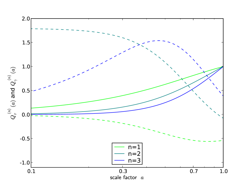
Figure 1: Time evolution functions Qγ(n)(a)superscriptsubscript𝑄𝛾𝑛𝑎Q_{\gamma}^{(n)}(a) (solid lines) and Qτ(n)(a)superscriptsubscript𝑄𝜏𝑛𝑎Q_{\tau}^{(n)}(a) (dashed lines) as a function of the scale factor a𝑎a for different perturbative orders n=1,2,3𝑛123n=1,2,3.

In Fig. 1 the time evolution functions Qγ(n)(a)superscriptsubscript𝑄𝛾𝑛𝑎Q_{\gamma}^{(n)}(a) and Qτ(n)(a)superscriptsubscript𝑄𝜏𝑛𝑎Q_{\tau}^{(n)}(a) are depicted in dependence on the scale factor a𝑎a. It is particularly interesting to observe the different signs. While the galaxy spectra are always positive, the iSW contributions change their signs with perturbative order. As we will later observe, also the signs of n𝑛n-point functions will change consequently in the transition from large scales, where the linear theory is valid, to small scales, where non-linearities start to dominate. For the cross-bispectrum, this effect has already been studied (Nishizawa et al., 2008).

3 MIXED BISPECTRA AND TRISPECTRA

3.1 The density polyspectra

Regardless of the existence of initial non-Gaussianities in the density field δ(𝐤)𝛿𝐤\delta(\mathbf{k}), non-linear structure formation leads to non-vanishing three-point and higher order correlators due to quadratic terms in the continuity and Euler equation. Since a Gaussian field can uniquely be represented by its two-point correlator ξ(r)=δ(𝐱)δ(𝐱+𝐫)𝜉𝑟delimited-⟨⟩𝛿𝐱𝛿𝐱𝐫\xi(r)=\langle\delta(\mathbf{x})\delta(\mathbf{x}+\mathbf{r})\rangle, multi-point correlators represent a convenient measure of evolving non-Gaussianities. The Fourier transforms of these 2-point and 3-point correlators are the bispectrum Bδ𝐤1,𝐤2,𝐤3superscriptsubscript𝐵𝛿subscript𝐤1subscript𝐤2subscript𝐤3B_{\delta}^{\,\mathbf{k}_{1},\mathbf{k}_{2},\mathbf{k}_{3}} and the trispectrum Tδ𝐤1,𝐤2,𝐤3,𝐤4superscriptsubscript𝑇𝛿subscript𝐤1subscript𝐤2subscript𝐤3subscript𝐤4T_{\delta}^{\,\mathbf{k}_{1},\mathbf{k}_{2},\mathbf{k}_{3},\mathbf{k}_{4}}

δ(𝐤1)δ(𝐤2)δ(𝐤3)delimited-⟨⟩𝛿subscript𝐤1𝛿subscript𝐤2𝛿subscript𝐤3\displaystyle\langle\delta(\mathbf{k}_{1})\delta(\mathbf{k}_{2})\delta(\mathbf{k}_{3})\rangle =\displaystyle= (2π)3δD(𝐤13)Bδ𝐤1,𝐤2,𝐤3superscript2𝜋3subscript𝛿Dsubscript𝐤13superscriptsubscript𝐵𝛿subscript𝐤1subscript𝐤2subscript𝐤3\displaystyle(2\pi)^{3}\delta_{\mathrm{D}}(\mathbf{k}_{1...3})\,B_{\delta}^{\,\mathbf{k}_{1},\mathbf{k}_{2},\mathbf{k}_{3}}
δ(𝐤1)δ(𝐤2)δ(𝐤3)δ(𝐤4)csubscriptdelimited-⟨⟩𝛿subscript𝐤1𝛿subscript𝐤2𝛿subscript𝐤3𝛿subscript𝐤4𝑐\displaystyle\langle\delta(\mathbf{k}_{1})\delta(\mathbf{k}_{2})\delta(\mathbf{k}_{3})\delta(\mathbf{k}_{4})\rangle_{c} =\displaystyle= (2π)3δD(𝐤14)Tδ𝐤1,𝐤2,𝐤3,𝐤4,superscript2𝜋3subscript𝛿Dsubscript𝐤14superscriptsubscript𝑇𝛿subscript𝐤1subscript𝐤2subscript𝐤3subscript𝐤4\displaystyle(2\pi)^{3}\delta_{\mathrm{D}}(\mathbf{k}_{1...4})\,T_{\delta}^{\,\mathbf{k}_{1},\mathbf{k}_{2},\mathbf{k}_{3},\mathbf{k}_{4}}\,, (26)

where the Dirac δDsubscript𝛿D\delta_{\mathrm{D}}-function is a result of homogeneity.

3.2 Limber Projection

In the flat sky approximation one can use a simplified Limber projection (Limber, 1953) to relate the 3-dimensional source spectra Bδ𝐤1,𝐤2,𝐤3superscriptsubscript𝐵𝛿subscript𝐤1subscript𝐤2subscript𝐤3B_{\delta}^{\,\mathbf{k}_{1},\mathbf{k}_{2},\mathbf{k}_{3}} and Tδ𝐤1,𝐤2,𝐤3,𝐤4superscriptsubscript𝑇𝛿subscript𝐤1subscript𝐤2subscript𝐤3subscript𝐤4T_{\delta}^{\,\mathbf{k}_{1},\mathbf{k}_{2},\mathbf{k}_{3},\mathbf{k}_{4}} to the angular spectra Bγ1,2,3superscriptsubscript𝐵𝛾subscriptbold-ℓ1subscriptbold-ℓ2subscriptbold-ℓ3B_{\gamma}^{\,\mn@boldsymbol{\ell}_{1},\mn@boldsymbol{\ell}_{2},\mn@boldsymbol{\ell}_{3}} and Tγ1,2,3,4superscriptsubscript𝑇𝛾subscriptbold-ℓ1subscriptbold-ℓ2subscriptbold-ℓ3subscriptbold-ℓ4T_{\gamma}^{\,\mn@boldsymbol{\ell}_{1},\mn@boldsymbol{\ell}_{2},\mn@boldsymbol{\ell}_{3},\mn@boldsymbol{\ell}_{4}}.

Bγ1,2,3superscriptsubscript𝐵𝛾subscriptbold-ℓ1subscriptbold-ℓ2subscriptbold-ℓ3\displaystyle B_{\gamma}^{\,\mn@boldsymbol{\ell}_{1},\mn@boldsymbol{\ell}_{2},\mn@boldsymbol{\ell}_{3}} =\displaystyle= 0χHdχ1χ4Wγ3(χ)D+4(a)Bδ𝐤1,𝐤2,𝐤3superscriptsubscript0subscript𝜒𝐻differential-d𝜒1superscript𝜒4superscriptsubscript𝑊𝛾3𝜒superscriptsubscript𝐷4𝑎superscriptsubscript𝐵𝛿subscript𝐤1subscript𝐤2subscript𝐤3\displaystyle\int_{0}^{\chi_{H}}\mathrm{d}\chi\frac{1}{\chi^{4}}\,W_{\gamma}^{3}(\chi)\,D_{+}^{4}(a)B_{\delta}^{\,\mathbf{k}_{1},\mathbf{k}_{2},\mathbf{k}_{3}}
Tγ1,2,3,4superscriptsubscript𝑇𝛾subscriptbold-ℓ1subscriptbold-ℓ2subscriptbold-ℓ3subscriptbold-ℓ4\displaystyle T_{\gamma}^{\,\mn@boldsymbol{\ell}_{1},\mn@boldsymbol{\ell}_{2},\mn@boldsymbol{\ell}_{3},\mn@boldsymbol{\ell}_{4}} =\displaystyle= 0χHdχ1χ6Wγ4(χ)D+6(a)Tδ𝐤1,𝐤2,𝐤3,𝐤4.superscriptsubscript0subscript𝜒𝐻differential-d𝜒1superscript𝜒6superscriptsubscript𝑊𝛾4𝜒superscriptsubscript𝐷6𝑎superscriptsubscript𝑇𝛿subscript𝐤1subscript𝐤2subscript𝐤3subscript𝐤4\displaystyle\int_{0}^{\chi_{H}}\mathrm{d}\chi\frac{1}{\chi^{6}}\,W_{\gamma}^{4}(\chi)\,D_{+}^{6}(a)T_{\delta}^{\,\mathbf{k}_{1},\mathbf{k}_{2},\mathbf{k}_{3},\mathbf{k}_{4}}. (27)

Then, equivalent formulae as in eqn. (3.1) apply to these angular polyspectra, which are then related to the projected density field γ()𝛾bold-ℓ\gamma(\mn@boldsymbol{\ell}) with two-dimensional angular wave vectors isubscriptbold-ℓ𝑖\mn@boldsymbol{\ell}_{i}:

γ(1)γ(2)γ(3)delimited-⟨⟩𝛾subscriptbold-ℓ1𝛾subscriptbold-ℓ2𝛾subscriptbold-ℓ3\displaystyle\langle\gamma(\mn@boldsymbol{\ell}_{1})\gamma(\mn@boldsymbol{\ell}_{2})\gamma(\mn@boldsymbol{\ell}_{3})\rangle =\displaystyle= (2π)3δD(13)Bγ1,2,3superscript2𝜋3subscript𝛿Dsubscriptbold-ℓ13superscriptsubscript𝐵𝛾subscriptbold-ℓ1subscriptbold-ℓ2subscriptbold-ℓ3\displaystyle(2\pi)^{3}\delta_{\mathrm{D}}(\mn@boldsymbol{\ell}_{1...3})\,B_{\gamma}^{\,\mn@boldsymbol{\ell}_{1},\mn@boldsymbol{\ell}_{2},\mn@boldsymbol{\ell}_{3}}
γ(1)γ(2)γ(3)γ(4)delimited-⟨⟩𝛾subscriptbold-ℓ1𝛾subscriptbold-ℓ2𝛾subscriptbold-ℓ3𝛾subscriptbold-ℓ4\displaystyle\langle\gamma(\mn@boldsymbol{\ell}_{1})\gamma(\mn@boldsymbol{\ell}_{2})\gamma(\mn@boldsymbol{\ell}_{3})\gamma(\mn@boldsymbol{\ell}_{4})\rangle =\displaystyle= (2π)3δD(14)Tγ1,2,3,4,superscript2𝜋3subscript𝛿Dsubscriptbold-ℓ14superscriptsubscript𝑇𝛾subscriptbold-ℓ1subscriptbold-ℓ2subscriptbold-ℓ3subscriptbold-ℓ4\displaystyle(2\pi)^{3}\delta_{\mathrm{D}}(\mn@boldsymbol{\ell}_{1...4})\,T_{\gamma}^{\,\mn@boldsymbol{\ell}_{1},\mn@boldsymbol{\ell}_{2},\mn@boldsymbol{\ell}_{3},\mn@boldsymbol{\ell}_{4}}\,, (28)

where the fields on the sphere with angular directions 𝐧isubscript𝐧𝑖\mathbf{n}_{i} are simply decomposed into Fourier harmonics instead of spherical harmonics

γ(𝐧1)γ(𝐧n)delimited-⟨⟩𝛾subscript𝐧1𝛾subscript𝐧𝑛\displaystyle\langle\gamma(\mathbf{n}_{1})...\gamma(\mathbf{n}_{n})\rangle =\displaystyle= d21(2π)2d2n(2π)2superscriptd2subscript1superscript2𝜋2superscriptd2subscript𝑛superscript2𝜋2\displaystyle\int\frac{\mathrm{d}^{2}\ell_{1}}{(2\pi)^{2}}...\int\frac{\mathrm{d}^{2}\ell_{n}}{(2\pi)^{2}}
γ(1)γ(n)ei1𝐧1ein𝐧n.absentdelimited-⟨⟩𝛾subscriptbold-ℓ1𝛾subscriptbold-ℓ𝑛superscripte𝑖subscriptbold-ℓ1subscript𝐧1superscripte𝑖subscriptbold-ℓ𝑛subscript𝐧𝑛\displaystyle\cdot\,\langle\gamma(\mn@boldsymbol{\ell}_{1})...\gamma(\mn@boldsymbol{\ell}_{n})\rangle\,\mathrm{e}^{i\mn@boldsymbol{\ell}_{1}\cdot\mathbf{n}_{1}}\,...\,\mathrm{e}^{i\mn@boldsymbol{\ell}_{n}\cdot\mathbf{n}_{n}}\,. (29)

Since the region on a sphere around a certain point can for small angles be approximated by the tangential plane, this is a good approximation for high \ell-values. It can generally be transformed to the full sky representation with Wigner 3j-symbols (Hu, 2001).

3.3 Mixed iSW-galaxy polyspectra

An equivalent procedure of definitions as in the previous subsection can be applied to the iSW-fields τ()𝜏bold-ℓ\tau(\mn@boldsymbol{\ell}). However, due to the uncorrelated noise sources in the iSW and galaxy fields mixed spectra are of predominant interest to us. If there exists a chance to securely measure the iSW signal it will only work via its cross-correlation to the projected galaxy density field γ()𝛾bold-ℓ\gamma(\mn@boldsymbol{\ell}) in the cross power spectrum and higher order correlators.

To allow a compact definition of the mixed spectra we introduce a doublet field φi()subscript𝜑𝑖bold-ℓ\varphi_{i}(\mn@boldsymbol{\ell})

(φ0()φ1())=(γ()τ()).fragmentsφ0()fragmentsφ1()fragmentsγ()fragmentsτ()\left(\begin{tabular}[]{r}$\varphi_{0}(\mn@boldsymbol{\ell})$\\ $\varphi_{1}(\mn@boldsymbol{\ell})$\end{tabular}\right)=\left(\begin{tabular}[]{c}$\gamma\,(\mn@boldsymbol{\ell})$\\ $\tau\,(\mn@boldsymbol{\ell})$\end{tabular}\right)\,. (30)

Mixed spectra can now be defined in a compact way

φi1(1)φi2(2)φi3(3)delimited-⟨⟩subscript𝜑subscript𝑖1subscriptbold-ℓ1subscript𝜑subscript𝑖2subscriptbold-ℓ2subscript𝜑subscript𝑖3subscriptbold-ℓ3\displaystyle\langle\varphi_{i_{1}}(\mn@boldsymbol{\ell}_{1})\varphi_{i_{2}}(\mn@boldsymbol{\ell}_{2})\varphi_{i_{3}}(\mn@boldsymbol{\ell}_{3})\rangle =\displaystyle= (2π)3δD(13)Bi1i2i31,2,3superscript2𝜋3subscript𝛿Dsubscriptbold-ℓ13superscriptsubscript𝐵subscript𝑖1subscript𝑖2subscript𝑖3subscriptbold-ℓ1subscriptbold-ℓ2subscriptbold-ℓ3\displaystyle(2\pi)^{3}\delta_{\mathrm{D}}(\mn@boldsymbol{\ell}_{1...3})\,B_{i_{1}i_{2}i_{3}}^{\,\mn@boldsymbol{\ell}_{1},\mn@boldsymbol{\ell}_{2},\mn@boldsymbol{\ell}_{3}}
φi1(1)φi2(2)φi3(3)φi4(4)delimited-⟨⟩subscript𝜑subscript𝑖1subscriptbold-ℓ1subscript𝜑subscript𝑖2subscriptbold-ℓ2subscript𝜑subscript𝑖3subscriptbold-ℓ3subscript𝜑subscript𝑖4subscriptbold-ℓ4\displaystyle\langle\varphi_{i_{1}}(\mn@boldsymbol{\ell}_{1})\varphi_{i_{2}}(\mn@boldsymbol{\ell}_{2})\varphi_{i_{3}}(\mn@boldsymbol{\ell}_{3})\varphi_{i_{4}}(\mn@boldsymbol{\ell}_{4})\rangle =\displaystyle= (2π)3δD(14)Ti1i2i3i41,2,3,4.superscript2𝜋3subscript𝛿Dsubscriptbold-ℓ14superscriptsubscript𝑇subscript𝑖1subscript𝑖2subscript𝑖3subscript𝑖4subscriptbold-ℓ1subscriptbold-ℓ2subscriptbold-ℓ3subscriptbold-ℓ4\displaystyle(2\pi)^{3}\delta_{\mathrm{D}}(\mn@boldsymbol{\ell}_{1...4})\,T_{i_{1}i_{2}i_{3}i_{4}}^{\,\mn@boldsymbol{\ell}_{1},\mn@boldsymbol{\ell}_{2},\mn@boldsymbol{\ell}_{3},\mn@boldsymbol{\ell}_{4}}. (31)

3.4 Weighting functions

For a mixed n𝑛n-point function, the product of the n𝑛n different weighting functions, is uniquely given by the sum of the field indices q𝑞q. In case of the bispectrum we would define q=i1+i2+i3𝑞subscript𝑖1subscript𝑖2subscript𝑖3q=i_{1}+i_{2}+i_{3}, whereas in case of the trispectrum q=i1+i2+i3+i4𝑞subscript𝑖1subscript𝑖2subscript𝑖3subscript𝑖4q=i_{1}+i_{2}+i_{3}+i_{4}. We can therefore define a q𝑞q-dependent combined weighting function Wq(n)(χ)superscriptsubscript𝑊𝑞𝑛𝜒W_{q}^{(n)}(\chi)

Wq(n)(χ)=Wτq(χ)Wγnq(χ)superscriptsubscript𝑊𝑞𝑛𝜒superscriptsubscript𝑊𝜏𝑞𝜒superscriptsubscript𝑊𝛾𝑛𝑞𝜒W_{q}^{(n)}(\chi)=W_{\tau}^{q}(\chi)W_{\gamma}^{n-q}(\chi)\, (32)

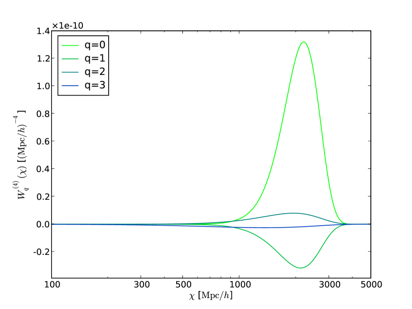
where n=3𝑛3n=3 and n=4𝑛4n=4 correspond to the bispectra and trispectra, respectively. The different weightings in case of the trispectra are depicted in Fig. 2 for different field mixtures q𝑞q. Despite the weightings show strong differences in amplitude and sign, common to all weightings is a broad peak between 1 and 4 Gpc h1superscript1h^{-1} due to the maximum in the galaxy redshift distribution p(z)𝑝𝑧p(z).

Refer to caption
Figure 2: Line-of-sight weighting functions Wq(4)(χ)superscriptsubscript𝑊𝑞4𝜒W_{q}^{(4)}(\chi) for mixed iSW-galaxy trispectra as a function of comoving distance.

3.5 Time evolution

The time evolution of each linear galaxy field γ(a,𝐤)𝛾𝑎𝐤\gamma(a,\mathbf{k}) is given by the growth function D+(a)subscript𝐷𝑎D_{+}(a). The n𝑛n-th non-linear perturbative contributions evolve simply with the n𝑛n-th order of the growth function D+nsuperscriptsubscript𝐷𝑛D_{+}^{n}. This is not the case for the iSW field contributions τ(a,𝐤)𝜏𝑎𝐤\tau(a,\mathbf{k}). While the linear term evolves proportional to d(D+/a)/dadsubscript𝐷𝑎d𝑎\mathrm{d}(D_{+}/a)/\mathrm{d}a the higher orders can not just be written as the n𝑛n-th power of the linear growth but are proportional to d(D+n/a)/dadsuperscriptsubscript𝐷𝑛𝑎d𝑎\mathrm{d}(D_{+}^{n}/a)/\mathrm{d}a.

Due to this fact, different perturbative contributions to mixed bispectra and trispectra will in general not have the same time evolution. In order to obtain a compact notation we introduce the time evolution doublet to n𝑛n-th order 𝐐(n)(a)superscript𝐐𝑛𝑎\mathbf{Q}^{(n)}(a)

𝐐(n)(a)=(Q0(n)(a)Q1(n)(a))=(D+ndda(D+na)).superscript𝐐𝑛𝑎fragmentsQ0𝑛(a)fragmentsQ1𝑛(a)fragmentsD𝑛fragmentsdd𝑎(superscriptsubscript𝐷𝑛𝑎)\mathbf{Q}^{(n)}(a)=\left(\begin{tabular}[]{r}$Q_{0}^{(n)}(a)$\\ $Q_{1}^{(n)}(a)$\end{tabular}\right)=\left(\begin{tabular}[]{c}$D_{+}^{n}$\\ $\frac{\mathrm{d}}{\mathrm{d}a}\left(\frac{D_{+}^{n}}{a}\right)$\end{tabular}\right)\,. (33)

With these time evolution functions 𝐐(n)(a)superscript𝐐𝑛𝑎\mathbf{Q}^{(n)}(a) we are now able to write down the general mixed time evolving source fields. For the tree-level bispectra we define

Bi1i2i3𝐤1,𝐤2,𝐤3superscriptsubscript𝐵subscript𝑖1subscript𝑖2subscript𝑖3subscript𝐤1subscript𝐤2subscript𝐤3\displaystyle B_{i_{1}i_{2}i_{3}}^{\,\mathbf{k}_{1},\mathbf{k}_{2},\mathbf{k}_{3}} =\displaystyle= (χHk1)2i1(χHk2)2i2(χHk3)2i3superscriptsubscript𝜒𝐻subscript𝑘12subscript𝑖1superscriptsubscript𝜒𝐻subscript𝑘22subscript𝑖2superscriptsubscript𝜒𝐻subscript𝑘32subscript𝑖3\displaystyle(\chi_{H}\,k_{1})^{-2i_{1}}(\chi_{H}\,k_{2})^{-2i_{2}}(\chi_{H}\,k_{3})^{-2i_{3}}
(Qi1(2)(a)Qi2(1)(a)Qi3(1)(a)bδ𝐤2,𝐤3\displaystyle\left(\,\,~{}Q_{i_{1}}^{(2)}(a)\,Q_{i_{2}}^{(1)}(a)\,Q_{i_{3}}^{(1)}(a)\,b_{\delta}^{\,\mathbf{k}_{2},\mathbf{k}_{3}}\right.
+Qi2(2)(a)Qi3(1)(a)Qi1(1)(a)bδ𝐤3,𝐤1superscriptsubscript𝑄subscript𝑖22𝑎superscriptsubscript𝑄subscript𝑖31𝑎superscriptsubscript𝑄subscript𝑖11𝑎superscriptsubscript𝑏𝛿subscript𝐤3subscript𝐤1\displaystyle\,\,+Q_{i_{2}}^{(2)}(a)\,Q_{i_{3}}^{(1)}(a)\,Q_{i_{1}}^{(1)}(a)\,b_{\delta}^{\,\mathbf{k}_{3},\mathbf{k}_{1}}
+Qi3(2)(a)Qi1(1)(a)Qi2(1)(a)bδ𝐤1,𝐤2).\displaystyle\,\,\left.+Q_{i_{3}}^{(2)}(a)\,Q_{i_{1}}^{(1)}(a)\,Q_{i_{2}}^{(1)}(a)\,b_{\delta}^{\,\mathbf{k}_{1},\mathbf{k}_{2}}\,\,\right)\,. (34)

The terms (χHk1)2isuperscriptsubscript𝜒𝐻subscript𝑘12𝑖(\chi_{H}\,k_{1})^{-2i} are the Poisson factors from the iSW effect. In case of the tree-level trispectrum the source will consist of two contributions - one originating from second order and third order perturbation theory respectively. The time dependent source for the trispectra then reads

Ti1i2i3i3𝐤1,𝐤2,𝐤3,𝐤3superscriptsubscript𝑇subscript𝑖1subscript𝑖2subscript𝑖3subscript𝑖3subscript𝐤1subscript𝐤2subscript𝐤3subscript𝐤3\displaystyle T_{i_{1}i_{2}i_{3}i_{3}}^{\,\mathbf{k}_{1},\mathbf{k}_{2},\mathbf{k}_{3},\mathbf{k}_{3}} =\displaystyle= (χHk1)2i1(χHk2)2i2(χHk3)2i3(χHk4)2i4superscriptsubscript𝜒𝐻subscript𝑘12subscript𝑖1superscriptsubscript𝜒𝐻subscript𝑘22subscript𝑖2superscriptsubscript𝜒𝐻subscript𝑘32subscript𝑖3superscriptsubscript𝜒𝐻subscript𝑘42subscript𝑖4\displaystyle(\chi_{H}\,k_{1})^{-2i_{1}}(\chi_{H}\,k_{2})^{-2i_{2}}(\chi_{H}\,k_{3})^{-2i_{3}}(\chi_{H}\,k_{4})^{-2i_{4}}
(Qi1(2)(a)Qi2(2)(a)Qi3(1)(a)Qi4(1)(a)tδ(2)(𝐤1,𝐤2),(𝐤3,𝐤4)\displaystyle\left(~{}Q_{i_{1}}^{(2)}(a)\,Q_{i_{2}}^{(2)}(a)\,Q_{i_{3}}^{(1)}(a)\,Q_{i_{4}}^{(1)}(a)\,t_{\delta}^{(2)\,(\mathbf{k}_{1},\mathbf{k}_{2}),(\mathbf{k}_{3},\mathbf{k}_{4})}\right.
+all pairs{1,2,3,4}all pairs1234\displaystyle+\,\hbox{all pairs}\,\in\,\{1,2,3,4\}
+Qi1(3)(a)Qi2(1)(a)Qi3(1)(a)Qi4(1)(a)tδ(3)(𝐤1,𝐤2,𝐤3,𝐤4)superscriptsubscript𝑄subscript𝑖13𝑎superscriptsubscript𝑄subscript𝑖21𝑎superscriptsubscript𝑄subscript𝑖31𝑎superscriptsubscript𝑄subscript𝑖41𝑎superscriptsubscript𝑡𝛿3subscript𝐤1subscript𝐤2subscript𝐤3subscript𝐤4\displaystyle+\,Q_{i_{1}}^{(3)}(a)\,Q_{i_{2}}^{(1)}(a)\,Q_{i_{3}}^{(1)}(a)\,Q_{i_{4}}^{(1)}(a)\,t_{\delta}^{(3)\,(\mathbf{k}_{1},\mathbf{k}_{2},\mathbf{k}_{3},\mathbf{k}_{4})}
+cyclic{1, 2, 3, 4}).\displaystyle\left.+\,\mathrm{cyclic}\,\{1,\,2,\,3,\,4\}~{}~{}\right)\,. (35)

Now, the flat sky Limber equations for the mixed angular bispectra and trispectra read (Hu, 2001)

Bi1i2i31,2,3superscriptsubscript𝐵subscript𝑖1subscript𝑖2subscript𝑖3subscriptbold-ℓ1subscriptbold-ℓ2subscriptbold-ℓ3\displaystyle B_{i_{1}i_{2}i_{3}}^{\,\mn@boldsymbol{\ell}_{1},\mn@boldsymbol{\ell}_{2},\mn@boldsymbol{\ell}_{3}} =\displaystyle= 0χHdχ1χ4Wq(3)(χ)Bi1i2i3𝐤1,𝐤2,𝐤3superscriptsubscript0subscript𝜒𝐻differential-d𝜒1superscript𝜒4superscriptsubscript𝑊𝑞3𝜒superscriptsubscript𝐵subscript𝑖1subscript𝑖2subscript𝑖3subscript𝐤1subscript𝐤2subscript𝐤3\displaystyle\int_{0}^{\chi_{H}}\mathrm{d}\chi\frac{1}{\chi^{4}}\,W_{q}^{(3)}(\chi)\,B_{i_{1}i_{2}i_{3}}^{\,\mathbf{k}_{1},\mathbf{k}_{2},\mathbf{k}_{3}}
Ti1i2i3i41,2,3,4superscriptsubscript𝑇subscript𝑖1subscript𝑖2subscript𝑖3subscript𝑖4subscriptbold-ℓ1subscriptbold-ℓ2subscriptbold-ℓ3subscriptbold-ℓ4\displaystyle T_{i_{1}i_{2}i_{3}i_{4}}^{\,\mn@boldsymbol{\ell}_{1},\mn@boldsymbol{\ell}_{2},\mn@boldsymbol{\ell}_{3},\mn@boldsymbol{\ell}_{4}} =\displaystyle= 0χHdχ1χ6Wq(4)(χ)Ti1i2i3i4𝐤1,𝐤2,𝐤3,𝐤4,superscriptsubscript0subscript𝜒𝐻differential-d𝜒1superscript𝜒6superscriptsubscript𝑊𝑞4𝜒superscriptsubscript𝑇subscript𝑖1subscript𝑖2subscript𝑖3subscript𝑖4subscript𝐤1subscript𝐤2subscript𝐤3subscript𝐤4\displaystyle\int_{0}^{\chi_{H}}\mathrm{d}\chi\frac{1}{\chi^{6}}\,W_{q}^{(4)}(\chi)\,T_{i_{1}i_{2}i_{3}i_{4}}^{\,\mathbf{k}_{1},\mathbf{k}_{2},\mathbf{k}_{3},\mathbf{k}_{4}}, (36)

where the source field spectra are evaluated at the 3-dimensional wave vectors 𝐤i=(li,1,li,2,0)subscript𝐤𝑖subscript𝑙𝑖1subscript𝑙𝑖20\mathbf{k}_{i}=(l_{i,1},l_{i,2},0). Since the weighting functions are slowly varying in comparison to the source field, fluctuations in the line-of-sight direction are smeared out by the integrations. Therefore, the fields can be assumed as non-fluctuating in this direction in the first place.

While pure spectra are invariant under exchange of wave vectors isubscriptbold-ℓ𝑖\mn@boldsymbol{\ell}_{i},

Baaa1,2,3superscriptsubscript𝐵𝑎𝑎𝑎subscriptbold-ℓ1subscriptbold-ℓ2subscriptbold-ℓ3\displaystyle B_{aaa}^{\,\mn@boldsymbol{\ell}_{1},\mn@boldsymbol{\ell}_{2},\mn@boldsymbol{\ell}_{3}} =\displaystyle= Baaa2,3,1=Baaa3,1,2superscriptsubscript𝐵𝑎𝑎𝑎subscriptbold-ℓ2subscriptbold-ℓ3subscriptbold-ℓ1superscriptsubscript𝐵𝑎𝑎𝑎subscriptbold-ℓ3subscriptbold-ℓ1subscriptbold-ℓ2\displaystyle B_{aaa}^{\,\mn@boldsymbol{\ell}_{2},\mn@boldsymbol{\ell}_{3},\mn@boldsymbol{\ell}_{1}}=B_{aaa}^{\,\mn@boldsymbol{\ell}_{3},\mn@boldsymbol{\ell}_{1},\mn@boldsymbol{\ell}_{2}}
Taaaa1,2,3,4superscriptsubscript𝑇𝑎𝑎𝑎𝑎subscriptbold-ℓ1subscriptbold-ℓ2subscriptbold-ℓ3subscriptbold-ℓ4\displaystyle T_{aaaa}^{\,\mn@boldsymbol{\ell}_{1},\mn@boldsymbol{\ell}_{2},\mn@boldsymbol{\ell}_{3},\mn@boldsymbol{\ell}_{4}} =\displaystyle= Taaaa2,3,4,1=Taaaa3,4,1,2=Taaaa4,1,2,3,superscriptsubscript𝑇𝑎𝑎𝑎𝑎subscriptbold-ℓ2subscriptbold-ℓ3subscriptbold-ℓ4subscriptbold-ℓ1superscriptsubscript𝑇𝑎𝑎𝑎𝑎subscriptbold-ℓ3subscriptbold-ℓ4subscriptbold-ℓ1subscriptbold-ℓ2superscriptsubscript𝑇𝑎𝑎𝑎𝑎subscriptbold-ℓ4subscriptbold-ℓ1subscriptbold-ℓ2subscriptbold-ℓ3\displaystyle T_{aaaa}^{\,\mn@boldsymbol{\ell}_{2},\mn@boldsymbol{\ell}_{3},\mn@boldsymbol{\ell}_{4},\mn@boldsymbol{\ell}_{1}}=T_{aaaa}^{\,\mn@boldsymbol{\ell}_{3},\mn@boldsymbol{\ell}_{4},\mn@boldsymbol{\ell}_{1},\mn@boldsymbol{\ell}_{2}}=T_{aaaa}^{\,\mn@boldsymbol{\ell}_{4},\mn@boldsymbol{\ell}_{1},\mn@boldsymbol{\ell}_{2},\mn@boldsymbol{\ell}_{3}}\,, (37)

this does not generally hold true for mixed spectra Babca,b,csuperscriptsubscript𝐵𝑎𝑏𝑐subscriptbold-ℓ𝑎subscriptbold-ℓ𝑏subscriptbold-ℓ𝑐B_{abc}^{\,\mn@boldsymbol{\ell}_{a},\mn@boldsymbol{\ell}_{b},\mn@boldsymbol{\ell}_{c}}. However, in general, all spectra are invariant under a simultaneous exchange of wave numbers and field indices

Bi1i2i31,2,3superscriptsubscript𝐵subscript𝑖1subscript𝑖2subscript𝑖3subscriptbold-ℓ1subscriptbold-ℓ2subscriptbold-ℓ3\displaystyle B_{i_{1}i_{2}i_{3}}^{\,\mn@boldsymbol{\ell}_{1},\mn@boldsymbol{\ell}_{2},\mn@boldsymbol{\ell}_{3}} =\displaystyle= Bi2i3i12,3,1=Bi3i1i23,1,2superscriptsubscript𝐵subscript𝑖2subscript𝑖3subscript𝑖1subscriptbold-ℓ2subscriptbold-ℓ3subscriptbold-ℓ1superscriptsubscript𝐵subscript𝑖3subscript𝑖1subscript𝑖2subscriptbold-ℓ3subscriptbold-ℓ1subscriptbold-ℓ2\displaystyle B_{i_{2}i_{3}i_{1}}^{\,\mn@boldsymbol{\ell}_{2},\mn@boldsymbol{\ell}_{3},\mn@boldsymbol{\ell}_{1}}=B_{i_{3}i_{1}i_{2}}^{\,\mn@boldsymbol{\ell}_{3},\mn@boldsymbol{\ell}_{1},\mn@boldsymbol{\ell}_{2}}
Ti1i2i3i41,2,3,4superscriptsubscript𝑇subscript𝑖1subscript𝑖2subscript𝑖3subscript𝑖4subscriptbold-ℓ1subscriptbold-ℓ2subscriptbold-ℓ3subscriptbold-ℓ4\displaystyle T_{i_{1}i_{2}i_{3}i_{4}}^{\,\mn@boldsymbol{\ell}_{1},\mn@boldsymbol{\ell}_{2},\mn@boldsymbol{\ell}_{3},\mn@boldsymbol{\ell}_{4}} =\displaystyle= Ti2i3i4i12,3,4,1=Ti3i4i1i23,4,1,2=Ti4i1i2i34,1,2,3.superscriptsubscript𝑇subscript𝑖2subscript𝑖3subscript𝑖4subscript𝑖1subscriptbold-ℓ2subscriptbold-ℓ3subscriptbold-ℓ4subscriptbold-ℓ1superscriptsubscript𝑇subscript𝑖3subscript𝑖4subscript𝑖1subscript𝑖2subscriptbold-ℓ3subscriptbold-ℓ4subscriptbold-ℓ1subscriptbold-ℓ2superscriptsubscript𝑇subscript𝑖4subscript𝑖1subscript𝑖2subscript𝑖3subscriptbold-ℓ4subscriptbold-ℓ1subscriptbold-ℓ2subscriptbold-ℓ3\displaystyle T_{i_{2}i_{3}i_{4}i_{1}}^{\,\mn@boldsymbol{\ell}_{2},\mn@boldsymbol{\ell}_{3},\mn@boldsymbol{\ell}_{4},\mn@boldsymbol{\ell}_{1}}=T_{i_{3}i_{4}i_{1}i_{2}}^{\,\mn@boldsymbol{\ell}_{3},\mn@boldsymbol{\ell}_{4},\mn@boldsymbol{\ell}_{1},\mn@boldsymbol{\ell}_{2}}=T_{i_{4}i_{1}i_{2}i_{3}}^{\,\mn@boldsymbol{\ell}_{4},\mn@boldsymbol{\ell}_{1},\mn@boldsymbol{\ell}_{2},\mn@boldsymbol{\ell}_{3}}\,. (38)

These symmetries are simply caused by the commutation invariance in the products of source fields in eqn. (3.1).

3.6 Equilateral bispectra and square trispectra

To require homogeneity the wave vector arguments have to form a triangle, 1+2+3=0subscriptbold-ℓ1subscriptbold-ℓ2subscriptbold-ℓ30\mn@boldsymbol{\ell}_{1}+\mn@boldsymbol{\ell}_{2}+\mn@boldsymbol{\ell}_{3}=0, for the bispectrum and a quadrangle, 1+2+3+4=0subscriptbold-ℓ1subscriptbold-ℓ2subscriptbold-ℓ3subscriptbold-ℓ40\mn@boldsymbol{\ell}_{1}+\mn@boldsymbol{\ell}_{2}+\mn@boldsymbol{\ell}_{3}+\mn@boldsymbol{\ell}_{4}=0, in case of the trispectrum. Thus, due to isotropy the scale dependence of the bispectrum is uniquely defined by the absolute values of the angular wave vectors isubscriptbold-ℓ𝑖\mn@boldsymbol{\ell}_{i}

Babca,b,c=Babca,b,c.superscriptsubscript𝐵𝑎𝑏𝑐subscriptbold-ℓ𝑎subscriptbold-ℓ𝑏subscriptbold-ℓ𝑐superscriptsubscript𝐵𝑎𝑏𝑐subscript𝑎subscript𝑏subscript𝑐B_{abc}^{\,\mn@boldsymbol{\ell}_{a},\mn@boldsymbol{\ell}_{b},\mn@boldsymbol{\ell}_{c}}=B_{abc}^{\,\ell_{a},\ell_{b},\ell_{c}}\,. (39)

The scale dependence of the trispectra, however, can be described by the four absolute values of the angular wave vectors isubscriptbold-ℓ𝑖\mn@boldsymbol{\ell}_{i} and one diagonal L𝐿L

Tabca,b,c,d=Tabca,b,c,d,L.superscriptsubscript𝑇𝑎𝑏𝑐subscriptbold-ℓ𝑎subscriptbold-ℓ𝑏subscriptbold-ℓ𝑐subscriptbold-ℓ𝑑superscriptsubscript𝑇𝑎𝑏𝑐subscript𝑎subscript𝑏subscript𝑐subscript𝑑𝐿T_{abc}^{\,\mn@boldsymbol{\ell}_{a},\mn@boldsymbol{\ell}_{b},\mn@boldsymbol{\ell}_{c},\mn@boldsymbol{\ell}_{d}}=T_{abc}^{\,\ell_{a},\ell_{b},\ell_{c},\ell_{d},L}\,. (40)

This leads to the fact that the source fields of equilateral bispectra are symmetric with respect to their field indices and have a uniform time evolution Qq,equi(a)subscript𝑄𝑞equi𝑎Q_{q,\mathrm{equi}}(a)

Qq,equi={D+3(q=0)13D+2(ddaD+2a)+23D+3(ddaD+a)(q=1)23D+(ddaD+2a)(ddaD+a)+13D+2(ddaD+a)2(q=2)(ddaD+2a)(ddaD+a)2(q=3).Q_{q,\mathrm{equi}}=\left\{\begin{tabular}[]{lcl}$D_{+}^{3}$&$(q=0)$&\\ $\frac{1}{3}D_{+}^{2}\left(\frac{\mathrm{d}}{\mathrm{d}a}\frac{D_{+}^{2}}{a}\right)+\frac{2}{3}D_{+}^{3}\left(\frac{\mathrm{d}}{\mathrm{d}a}\frac{D_{+}}{a}\right)$&$(q=1)$&\\ $\frac{2}{3}D_{+}\left(\frac{\mathrm{d}}{\mathrm{d}a}\frac{D_{+}^{2}}{a}\right)\left(\frac{\mathrm{d}}{\mathrm{d}a}\frac{D_{+}}{a}\right)+\frac{1}{3}D_{+}^{2}\left(\frac{\mathrm{d}}{\mathrm{d}a}\frac{D_{+}}{a}\right)^{2}$&$(q=2)$&\\ $\left(\frac{\mathrm{d}}{\mathrm{d}a}\frac{D_{+}^{2}}{a}\right)\left(\frac{\mathrm{d}}{\mathrm{d}a}\frac{D_{+}}{a}\right)^{2}$&$(q=3)$&\,.\\ \end{tabular}\right. (41)

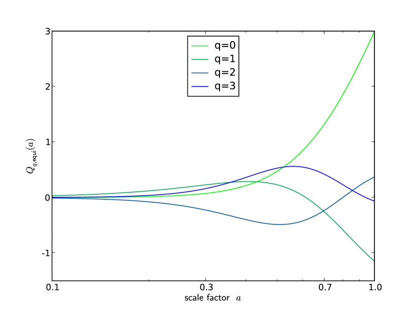
These time evolutions are depicted in Fig. 3. While the growth functions of the galaxy distribution stay positive to all perturbative orders, the derivatives in the iSW evolution functions also introduce negative terms into the evolution. This will later lead to a change from correlation to anti-correlation along the line-of-sight.
Refer to caption
Figure 3: Time evolution functions for equilateral mixed iSW-galaxy bispectra Bi1i2i3,,superscriptsubscript𝐵subscript𝑖1subscript𝑖2subscript𝑖3B_{i_{1}i_{2}i_{3}}^{\,\ell,\ell,\ell} as a function of angular scale \ell. The value q=i1+i2+i3𝑞subscript𝑖1subscript𝑖2subscript𝑖3q=i_{1}+i_{2}+i_{3} defines the mixture of the source fields. While the growth functions of the galaxy distribution stay positive to all perturbative orders, the derivatives in the iSW evolution functions also introduce negative terms into the evolution.

Slightly more complex is the time evolution for source fields of the square trispectra. Here, the contributions from second order perturbation theory evolve still differently compared to the third order terms. The second order terms Qq,square(2)(a)superscriptsubscript𝑄𝑞square2𝑎Q_{q,\mathrm{square}}^{(2)}(a) read

Refer to caption
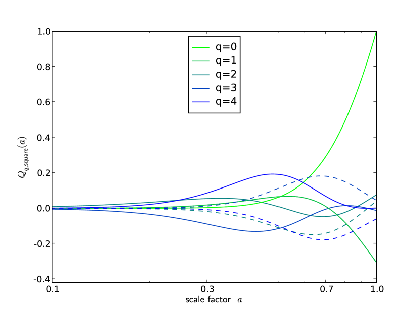
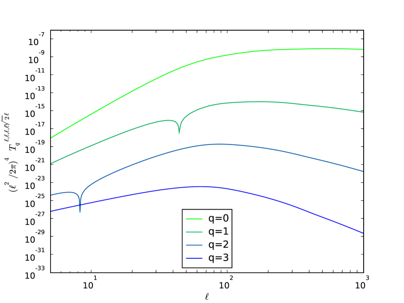
Figure 4: Time evolution functions for square mixed iSW-galaxy trispectra T(i1i2i3i4),,,,2superscriptsubscript𝑇subscript𝑖1subscript𝑖2subscript𝑖3subscript𝑖42T_{(i_{1}i_{2}i_{3}i_{4})}^{\,\ell,\ell,\ell,\ell,\sqrt{2}\ell} as a function of angular scale \ell. The value q=i1+i2+i3+i4𝑞subscript𝑖1subscript𝑖2subscript𝑖3subscript𝑖4q=i_{1}+i_{2}+i_{3}+i_{4} defines the mixture of the source fields. The solid lines depict the second order perturbative time evolutions Qq,square(2)superscriptsubscript𝑄𝑞square2Q_{q,\mathrm{square}}^{(2)}, the third order terms Qq,square(3)superscriptsubscript𝑄𝑞square3Q_{q,\mathrm{square}}^{(3)} are show as dashed lines. While the growth functions of the galaxy distribution stay positive to all perturbative orders, the derivatives in the iSW evolution functions also introduce negative terms into the evolution.
Qq,square(2)superscriptsubscript𝑄𝑞square2\displaystyle Q_{q,\mathrm{square}}^{(2)} ={D+6(q=0)12D+4(ddaD+2a)+12D+5(ddaD+a)(q=1)16D+4(ddaD+a)2+23D+3(ddaD+2a)(ddaD+a)+16D+2(ddaD+2a)2(q=2)12D+(ddaD+2a)2(ddaD+a)+12D+2(ddaD+2a)(ddaD+a)2(q=3)(ddaD+2a)2(ddaD+a)2(q=4)\displaystyle=\left\{\begin{tabular}[]{lcl}$D_{+}^{6}$&$(q=0)$&\\ $\frac{1}{2}D_{+}^{4}\left(\frac{\mathrm{d}}{\mathrm{d}a}\frac{D_{+}^{2}}{a}\right)+\frac{1}{2}D_{+}^{5}\left(\frac{\mathrm{d}}{\mathrm{d}a}\frac{D_{+}}{a}\right)$&$(q=1)$&\\ $\frac{1}{6}D_{+}^{4}\left(\frac{\mathrm{d}}{\mathrm{d}a}\frac{D_{+}}{a}\right)^{2}+\frac{2}{3}D_{+}^{3}\left(\frac{\mathrm{d}}{\mathrm{d}a}\frac{D_{+}^{2}}{a}\right)\left(\frac{\mathrm{d}}{\mathrm{d}a}\frac{D_{+}}{a}\right)$&{}\hfil&\\ $+\frac{1}{6}D_{+}^{2}\left(\frac{\mathrm{d}}{\mathrm{d}a}\frac{D_{+}^{2}}{a}\right)^{2}$&$(q=2)$&\\ $\frac{1}{2}D_{+}\left(\frac{\mathrm{d}}{\mathrm{d}a}\frac{D_{+}^{2}}{a}\right)^{2}\left(\frac{\mathrm{d}}{\mathrm{d}a}\frac{D_{+}}{a}\right)+\frac{1}{2}D_{+}^{2}\left(\frac{\mathrm{d}}{\mathrm{d}a}\frac{D_{+}^{2}}{a}\right)\left(\frac{\mathrm{d}}{\mathrm{d}a}\frac{D_{+}}{a}\right)^{2}$&$(q=3)$&\\ $\left(\frac{\mathrm{d}}{\mathrm{d}a}\frac{D_{+}^{2}}{a}\right)^{2}\left(\frac{\mathrm{d}}{\mathrm{d}a}\frac{D_{+}}{a}\right)^{2}$&$(q=4)$&\end{tabular}\right. (48)

and for the third order we obtain the following time evolution:

Qq,square(3)superscriptsubscript𝑄𝑞square3\displaystyle Q_{q,\mathrm{square}}^{(3)} ={D+6(q=0)14D+5(ddaD+a)+34D+3(ddaD+3a)(q=1)12D+4(ddaD+a)2+12D+2(ddaD+3a)(ddaD+a)(q=2)14D+3(ddaD+2a)3+34D+(ddaD+3a)(ddaD+a)2(q=3)(ddaD+3a)(ddaD+a)3(q=4).\displaystyle=\left\{\begin{tabular}[]{lcl}$D_{+}^{6}$&$(q=0)$&\\ $\frac{1}{4}D_{+}^{5}\left(\frac{\mathrm{d}}{\mathrm{d}a}\frac{D_{+}}{a}\right)+\frac{3}{4}D_{+}^{3}\left(\frac{\mathrm{d}}{\mathrm{d}a}\frac{D_{+}^{3}}{a}\right)$&$(q=1)$&\\ $\frac{1}{2}D_{+}^{4}\left(\frac{\mathrm{d}}{\mathrm{d}a}\frac{D_{+}}{a}\right)^{2}+\frac{1}{2}D_{+}^{2}\left(\frac{\mathrm{d}}{\mathrm{d}a}\frac{D_{+}^{3}}{a}\right)\left(\frac{\mathrm{d}}{\mathrm{d}a}\frac{D_{+}}{a}\right)$&$(q=2)$&\\ $\frac{1}{4}D_{+}^{3}\left(\frac{\mathrm{d}}{\mathrm{d}a}\frac{D_{+}^{2}}{a}\right)^{3}+\frac{3}{4}D_{+}\left(\frac{\mathrm{d}}{\mathrm{d}a}\frac{D_{+}^{3}}{a}\right)\left(\frac{\mathrm{d}}{\mathrm{d}a}\frac{D_{+}}{a}\right)^{2}$&$(q=3)$&\\ $\left(\frac{\mathrm{d}}{\mathrm{d}a}\frac{D_{+}^{3}}{a}\right)\left(\frac{\mathrm{d}}{\mathrm{d}a}\frac{D_{+}}{a}\right)^{3}$&$(q=4)$&\,.\end{tabular}\right. (54)

In time evolutions for the different perturbative orders of the mixed trispectra are depicted in Fig. 4. One can see that for q=1,2𝑞12q=1,2 they evolve identically but differ stronger with increasing number q𝑞q of included iSW fields.

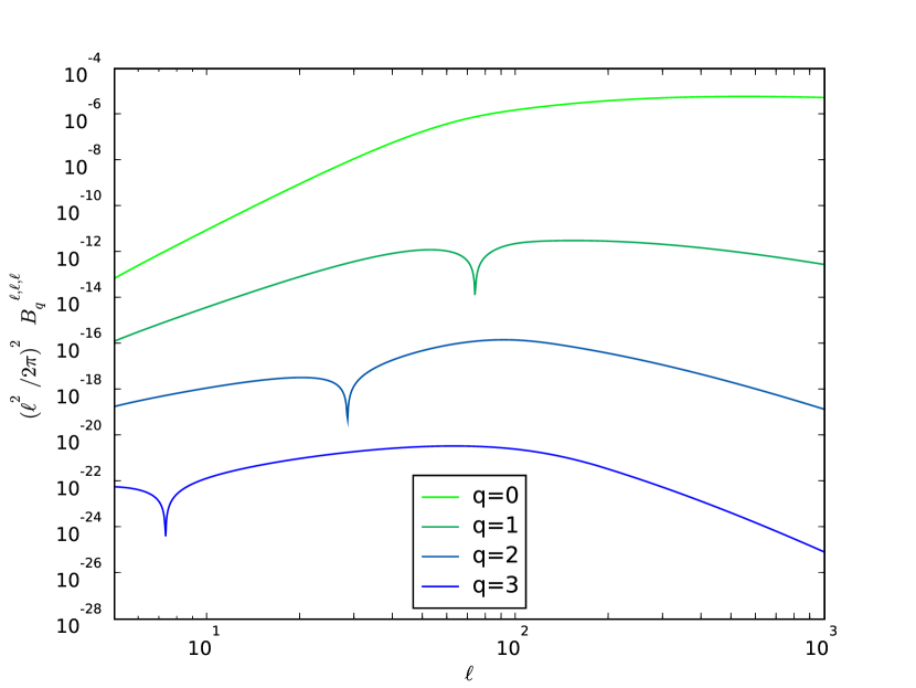
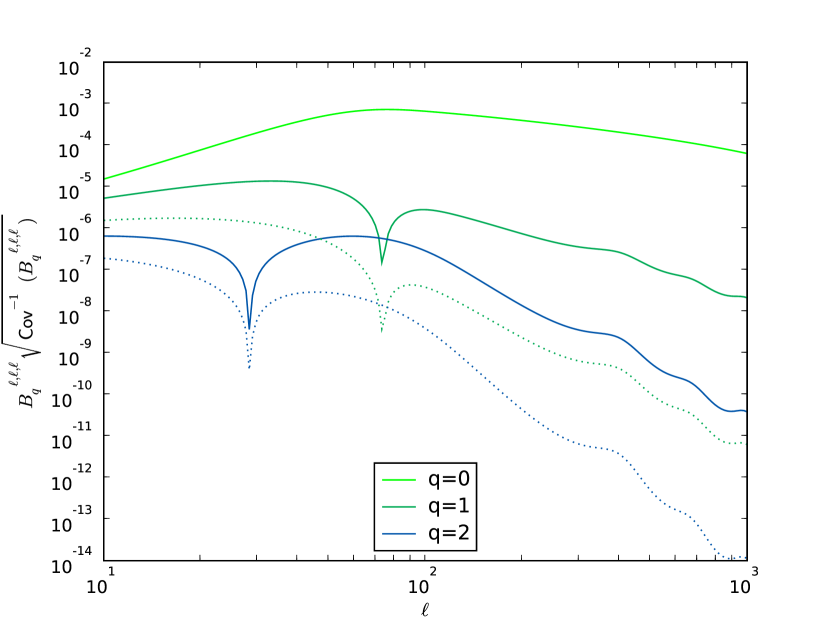
The equilateral bispectra and square trispectra are depicted in Fig. 5 and Fig. 6. As in the power spectra one can observe also here the weakness of the iSW signal in comparison to the projected galaxy distribution field. This is clearly shown in the decrease of the polyspectra with increasing number q𝑞q of included iSW source fields. Once more, the iSW effect shows its nature of being a large scale effect. With higher q𝑞q the slope of the spectra increases in the large \ell region. The physical reason for this is the coupling of the iSW effect to the gravitational potential in contrast to the galaxy distribution, which couples directly to the density contrast. Mathematically, this fact manifests itself in the appearance of the 1/k21superscript𝑘21/k^{2} factors for the iSW contributions, originating from the inversion of the Poisson equation.

While the linear iSW effect is strictly anti-correlated with respect to the galaxy density, cross-spectra with this linear signal would never show a change in sign in dependence on \ell. This does not hold true any longer for the non-linear iSW effect. The higher order contributions now have the opposite sign in their time evolution. It is therefore possible that for large \ell the linear effect dominates while for small \ell the non-linear effect determines the sign of the correlation. These changes in sign in dependence of \ell can now be observed in Fig. 5 and Fig. 6, for instance at 8080\ell\approx 80 in the bispectrum τγ2delimited-⟨⟩𝜏superscript𝛾2\langle\tau\gamma^{2}\rangle.

Refer to caption
Figure 5: The absolute values of the mixed equilateral iSW-galaxy bispectra Bi1i2i3,,superscriptsubscript𝐵subscript𝑖1subscript𝑖2subscript𝑖3B_{i_{1}i_{2}i_{3}}^{\,\ell,\ell,\ell} as a function of angular scale \ell are depicted in this figure. The value q=i1+i2+i3𝑞subscript𝑖1subscript𝑖2subscript𝑖3q=i_{1}+i_{2}+i_{3} defines the mixture of the source fields.
Refer to caption
Figure 6: The absolute values of the mixed square iSW-galaxy trispectra Ti1i2i3i4,,,,2superscriptsubscript𝑇subscript𝑖1subscript𝑖2subscript𝑖3subscript𝑖42T_{i_{1}i_{2}i_{3}i_{4}}^{\,\ell,\ell,\ell,\ell,\sqrt{2}\ell} as a function of angular scale \ell are shown in this plot. The value q=i1+i2+i3+i4𝑞subscript𝑖1subscript𝑖2subscript𝑖3subscript𝑖4q=i_{1}+i_{2}+i_{3}+i_{4} defines the mixture of the source fields.

This behavior has also been observed and studied in the CMB-weak-lensing cross spectrum (Nishizawa et al., 2008).

4 DETECTABILITY

4.1 Sources of noise

The step from a good theoretical framework to an analysis of real data or to an estimation of the realistically accessible information content encompasses the description of all relevant effects influencing the measured data. Only then, one will be able to make statements about a physical process and the likelihood of its actual measurement. For the evaluation of the covariances of the bispectra and trispectra, the two-point function will be needed. In the same notation as the higher order spectra their are defined as

φi1(1)φi2(2)=(2π)2δD(1+2)Ci1i21delimited-⟨⟩subscript𝜑subscript𝑖1subscriptbold-ℓ1subscript𝜑subscript𝑖2subscriptbold-ℓ2superscript2𝜋2subscript𝛿Dsubscriptbold-ℓ1subscriptbold-ℓ2superscriptsubscript𝐶subscript𝑖1subscript𝑖2subscript1\langle\varphi_{i_{1}}(\mn@boldsymbol{\ell}_{1})\varphi_{i_{2}}(\mn@boldsymbol{\ell}_{2})\rangle=(2\pi)^{2}\delta_{\mathrm{D}}(\mn@boldsymbol{\ell}_{1}+\mn@boldsymbol{\ell}_{2})\,C_{i_{1}i_{2}}^{\ell_{1}} (55)

In the case at hand the actual theoretically expected iSW signal in our fiducial cosmological model is superposed to the primary CMB fluctuations. Its relative amplitude reaches from 10%percent\% on very large scales to an negligible fraction of the signal for scales smaller than 200200\ell\approx 200. Furthermore, the detected CMB signal is subjected to instrumental noise στsubscript𝜎𝜏\sigma_{\tau} and a Gaussian beam β()𝛽\beta(\ell).

Assuming that the noise sources of the galaxy counts are mutually uncorrelated, the pure galaxy-galaxy spectra are solely subjected to a Poissonian noise term n1superscript𝑛1n^{-1}.

The cross-spectra between the two fields will be free of noise, since the noise sources of the single fields are uncorrelated.

Now we can relate the measured spectra C~i1i2superscriptsubscript~𝐶subscript𝑖1subscript𝑖2\tilde{C}_{i_{1}i_{2}}^{\ell} to the theoretical spectra C~i1i2superscriptsubscript~𝐶subscript𝑖1subscript𝑖2\tilde{C}_{i_{1}i_{2}}^{\ell}:

C~00superscriptsubscript~𝐶00\displaystyle\tilde{C}_{00}^{\ell} =\displaystyle= C00+n1superscriptsubscript𝐶00superscript𝑛1\displaystyle C_{00}^{\ell}+n^{-1}
C~01superscriptsubscript~𝐶01\displaystyle\tilde{C}_{01}^{\ell} =\displaystyle= C01superscriptsubscript𝐶01\displaystyle C_{01}^{\ell}
C~11superscriptsubscript~𝐶11\displaystyle\tilde{C}_{11}^{\ell} =\displaystyle= C11+CCMB+στ2β2().superscriptsubscript𝐶11superscriptsubscript𝐶CMBsuperscriptsubscript𝜎𝜏2superscript𝛽2\displaystyle C_{11}^{\ell}+C_{\mathrm{CMB}}^{\ell}+\sigma_{\tau}^{2}\,\beta^{-2}(\ell)\,. (56)

The contributions in detail are:

(i) As the Fourier transform of the Gaussian beam one obtains β2()=exp(Δθ2(+1))superscript𝛽2Δsuperscript𝜃21\beta^{-2}(\ell)=\exp(\Delta\theta^{2}\ell(\ell+1)). We use Δθ=7.1Δ𝜃7.1\Delta\theta=7.1 arcmin, which corresponds to the ν=143GHz𝜈143GHz\nu=143\,\,\mathrm{GHz} channels closest to the CMB emission maximum. For the conversion of wT1=TCMB2στ2superscriptsubscript𝑤𝑇1superscriptsubscript𝑇CMB2superscriptsubscript𝜎𝜏2w_{T}^{-1}=T_{\mathrm{CMB}}^{2}\sigma_{\tau}^{2} to the noise amplitude in the dimensionless temperature perturbation τ𝜏\tau with wT=(0.01μK)2subscript𝑤𝑇superscript0.01𝜇K2w_{T}=(0.01\,\,\mu\mathrm{K})^{2} (Zaldarriaga et al., 1997) we use the value TCMB=2.725Ksubscript𝑇CMB2.725KT_{\mathrm{CMB}}=2.725\,\,\mathrm{K} for the CMB temperature.

N𝑁N ΔΩΔΩ\Delta\Omega fskysubscript𝑓skyf_{\mathrm{sky}} z0subscript𝑧0z_{0} b𝑏b n𝑛n
3.0×1093.0superscript1093.0\times 10^{9} 2π2𝜋2\pi 0.50.50.5 0.640.640.64 1.01.01.0 4.7×1084.7superscript1084.7\times 10^{8}
Table 1: The Properties of the Euclid galaxy survey are listed in this table: total number N𝑁N of objects, solid angle ΔΩΔΩ\Delta\Omega covered (in radians), sky fraction fskysubscript𝑓skyf_{\mathrm{sky}}, redshift parameter z0subscript𝑧0z_{0}, galaxy bias b𝑏b and density per unit steradian n𝑛n.

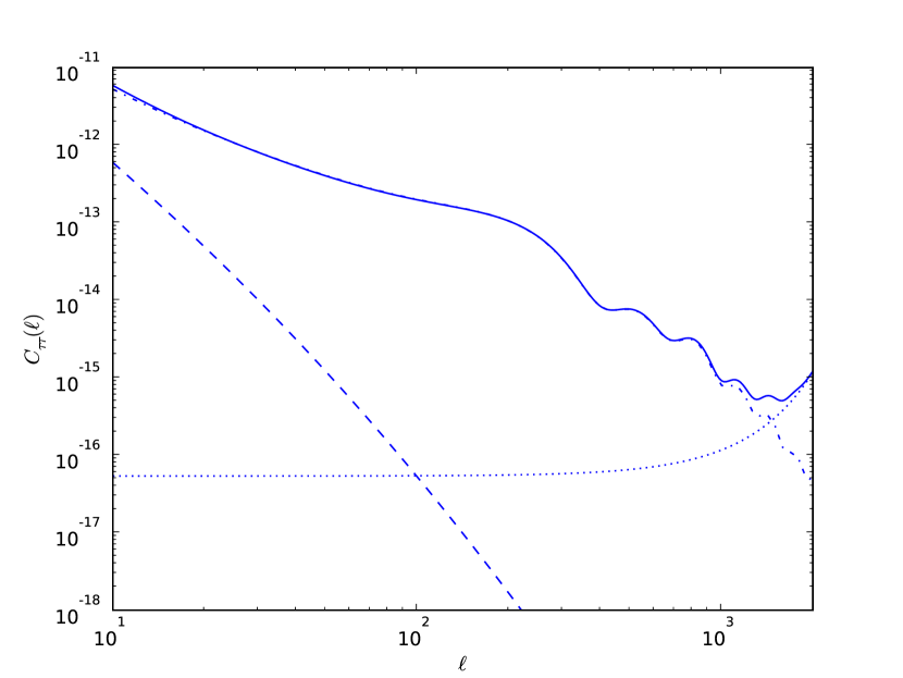
(ii) Furthermore, a CMB temperature power spectrum CCMB()subscript𝐶CMBC_{\mathrm{CMB}}(\ell) was generated, which was equally scaled with the CMB temperature TCMB=2.725Ksubscript𝑇CMB2.725KT_{\mathrm{CMB}}=2.725\,\,\mathrm{K}, with the Code for Anisotropies in the Microwave Background (CAMB, Lewis et al., 2000) for the fiducial ΛΛ\LambdaCDM cosmology. The noise contribution from the CMB-spectrum CCMBsuperscriptsubscript𝐶CMBC_{\mathrm{CMB}}^{\ell} represents the main challenge in the observation of the iSW bispectra and trispectra. It provides high values for the covariance at low multipoles \ell, and it by far dominates C~00()subscript~𝐶00\tilde{C}_{00}(\ell), CCMBC00()much-greater-thansubscript𝐶CMBsubscript𝐶00C_{\mathrm{CMB}}\gg C_{00}(\ell) on the angular scales considered. The orders of magnitude for the different contributions of the linear estimator C~11superscriptsubscript~𝐶11\tilde{C}_{11}^{\ell} are depicted in Fig 7. One can see, that even at large angular scales \ell the pure iSW signal C11superscriptsubscript𝐶11C_{11}^{\ell} is still more than one order of magnitude weaker than the signal from primordial fluctuations CCMBsuperscriptsubscript𝐶CMBC_{\mathrm{CMB}}^{\ell}.

Refer to caption
Figure 7: Constituents of the measured angular CMB spectrum C~11superscriptsubscript~𝐶11\tilde{C}_{11}^{\ell}. Depicted are the total signal C~11superscriptsubscript~𝐶11\tilde{C}_{11}^{\ell} (solid line), the contribution from primordial fluctuations CCMBsuperscriptsubscript𝐶CMBC_{\mathrm{CMB}}^{\ell}, the iSW-effect C11superscriptsubscript𝐶11C_{11}^{\ell} and the instrumental noise στ2β2()superscriptsubscript𝜎𝜏2superscript𝛽2\sigma_{\tau}^{2}\,\beta^{-2}(\ell), which is fortunately sub-dominant at the large scales of interest.

(iii) The inverse number density n𝑛n of objects per unit steradian determines the Poissonian noise term in the galaxy count. In Table 1 the properties of the main galaxy sample as it would be expected from Euclid are summarized. Major advantages lie in the large sky coverage and the high number of observed objects. Here, we assumed a non-evolving galaxy bias for simplicity.

4.2 Covariances

In the case of Gaussian noise the observed and estimated bispectra B~i1i2i31,2,3superscriptsubscript~𝐵subscript𝑖1subscript𝑖2subscript𝑖3subscript1subscript2subscript3\tilde{B}_{i_{1}i_{2}i_{3}}^{\,\ell_{1},\ell_{2},\ell_{3}} and the trispectra T~i1i2i3i41,2,3,4superscriptsubscript~𝑇subscript𝑖1subscript𝑖2subscript𝑖3subscript𝑖4subscriptbold-ℓ1subscriptbold-ℓ2subscriptbold-ℓ3subscriptbold-ℓ4\tilde{T}_{i_{1}i_{2}i_{3}i_{4}}^{\,\mn@boldsymbol{\ell}_{1},\mn@boldsymbol{\ell}_{2},\mn@boldsymbol{\ell}_{3},\mn@boldsymbol{\ell}_{4}} are unbiased estimates of the true bispectra Bi1i2i31,2,3superscriptsubscript𝐵subscript𝑖1subscript𝑖2subscript𝑖3subscript1subscript2subscript3B_{i_{1}i_{2}i_{3}}^{\,\ell_{1},\ell_{2},\ell_{3}} and trispectra Ti1i2i3i41,2,3,4superscriptsubscript𝑇subscript𝑖1subscript𝑖2subscript𝑖3subscript𝑖4subscriptbold-ℓ1subscriptbold-ℓ2subscriptbold-ℓ3subscriptbold-ℓ4T_{i_{1}i_{2}i_{3}i_{4}}^{\,\mn@boldsymbol{\ell}_{1},\mn@boldsymbol{\ell}_{2},\mn@boldsymbol{\ell}_{3},\mn@boldsymbol{\ell}_{4}} (Hu, 2001),

B~i1i2i31,2,3superscriptsubscript~𝐵subscript𝑖1subscript𝑖2subscript𝑖3subscript1subscript2subscript3\displaystyle\tilde{B}_{i_{1}i_{2}i_{3}}^{\,\ell_{1},\ell_{2},\ell_{3}} similar-to-or-equals\displaystyle\simeq Bi1i2i31,2,3superscriptsubscript𝐵subscript𝑖1subscript𝑖2subscript𝑖3subscript1subscript2subscript3\displaystyle B_{i_{1}i_{2}i_{3}}^{\,\ell_{1},\ell_{2},\ell_{3}}
T~i1i2i3i41,2,3,4superscriptsubscript~𝑇subscript𝑖1subscript𝑖2subscript𝑖3subscript𝑖4subscriptbold-ℓ1subscriptbold-ℓ2subscriptbold-ℓ3subscriptbold-ℓ4\displaystyle\tilde{T}_{i_{1}i_{2}i_{3}i_{4}}^{\,\mn@boldsymbol{\ell}_{1},\mn@boldsymbol{\ell}_{2},\mn@boldsymbol{\ell}_{3},\mn@boldsymbol{\ell}_{4}} similar-to-or-equals\displaystyle\simeq Ti1i2i3i41,2,3,4.superscriptsubscript𝑇subscript𝑖1subscript𝑖2subscript𝑖3subscript𝑖4subscriptbold-ℓ1subscriptbold-ℓ2subscriptbold-ℓ3subscriptbold-ℓ4\displaystyle T_{i_{1}i_{2}i_{3}i_{4}}^{\,\mn@boldsymbol{\ell}_{1},\mn@boldsymbol{\ell}_{2},\mn@boldsymbol{\ell}_{3},\mn@boldsymbol{\ell}_{4}}\,. (57)

This is in contrast to the spectra Ci1i2superscriptsubscript𝐶subscript𝑖1subscript𝑖2C_{i_{1}i_{2}}^{\ell}, which were discussed in the previous subsection. The covariances of the estimators of the bispectra and trispectra are defined as

Cov[B~i1i2i31,2,3,B~i1i2i31,2,3]Covsuperscriptsubscript~𝐵subscript𝑖1subscript𝑖2subscript𝑖3subscript1subscript2subscript3superscriptsubscript~𝐵subscript𝑖1subscript𝑖2subscript𝑖3superscriptsubscript1superscriptsubscript2superscriptsubscript3\displaystyle\mathrm{Cov}\left[\tilde{B}_{i_{1}i_{2}i_{3}}^{\,\ell_{1},\ell_{2},\ell_{3}},\tilde{B}_{i_{1}i_{2}i_{3}}^{\,\ell_{1}^{\prime},\ell_{2}^{\prime},\ell_{3}^{\prime}}\right]\hskip 85.35826pt
=(B~i1i2i31,2,3Bi1i2i31,2,3)(B~i1i2i31,2,3Bi1i2i31,2,3),absentdelimited-⟨⟩superscriptsubscript~𝐵subscript𝑖1subscript𝑖2subscript𝑖3superscriptsubscript1absentsubscript2subscript3superscriptsubscript𝐵subscript𝑖1subscript𝑖2subscript𝑖3subscript1subscript2subscript3superscriptsubscript~𝐵subscript𝑖1subscript𝑖2subscript𝑖3superscriptsubscript1superscriptsubscript2superscriptsubscript3superscriptsubscript𝐵subscript𝑖1subscript𝑖2subscript𝑖3superscriptsubscript1superscriptsubscript2superscriptsubscript3\displaystyle=\left\langle\left(\tilde{B}_{i_{1}i_{2}i_{3}}^{\,\ell_{1}^{~{}},\ell_{2},\ell_{3}}-B_{i_{1}i_{2}i_{3}}^{\,\ell_{1},\ell_{2},\ell_{3}}\right)\right.\left.\left(\tilde{B}_{i_{1}i_{2}i_{3}}^{\,\ell_{1}^{\prime},\ell_{2}^{\prime},\ell_{3}^{\prime}}-B_{i_{1}i_{2}i_{3}}^{\,\ell_{1}^{\prime},\ell_{2}^{\prime},\ell_{3}^{\prime}}\right)\right\rangle\,,
Cov[T~i1i2i3,i41,2,3,4,T~i1i2i3,i41,2,3,4]Covsuperscriptsubscript~𝑇subscript𝑖1subscript𝑖2subscript𝑖3subscript𝑖4subscriptbold-ℓ1subscriptbold-ℓ2subscriptbold-ℓ3subscriptbold-ℓ4superscriptsubscript~𝑇subscript𝑖1subscript𝑖2subscript𝑖3subscript𝑖4superscriptsubscriptbold-ℓ1superscriptsubscriptbold-ℓ2superscriptsubscriptbold-ℓ3superscriptsubscriptbold-ℓ4\displaystyle\mathrm{Cov}\left[\tilde{T}_{i_{1}i_{2}i_{3},i_{4}}^{\,\mn@boldsymbol{\ell}_{1},\mn@boldsymbol{\ell}_{2},\mn@boldsymbol{\ell}_{3},\mn@boldsymbol{\ell}_{4}},\tilde{T}_{i_{1}i_{2}i_{3},i_{4}}^{\,\mn@boldsymbol{\ell}_{1}^{\prime},\mn@boldsymbol{\ell}_{2}^{\prime},\mn@boldsymbol{\ell}_{3}^{\prime},\mn@boldsymbol{\ell}_{4}^{\prime}}\right]\hskip 113.81102pt
=(T~i1i2i3,i41,2,3,4,LTi1i2i3,i41,2,3,4)(T~i1i2i3,i41,2,3,4Ti1i2i3,i41,2,3,4).absentdelimited-⟨⟩superscriptsubscript~𝑇subscript𝑖1subscript𝑖2subscript𝑖3subscript𝑖4superscriptsubscript1absentsubscript2subscript3subscript4𝐿superscriptsubscript𝑇subscript𝑖1subscript𝑖2subscript𝑖3subscript𝑖4subscriptbold-ℓ1subscriptbold-ℓ2subscriptbold-ℓ3subscriptbold-ℓ4superscriptsubscript~𝑇subscript𝑖1subscript𝑖2subscript𝑖3subscript𝑖4superscriptsubscriptbold-ℓ1superscriptsubscriptbold-ℓ2superscriptsubscriptbold-ℓ3superscriptsubscriptbold-ℓ4superscriptsubscript𝑇subscript𝑖1subscript𝑖2subscript𝑖3subscript𝑖4superscriptsubscriptbold-ℓ1superscriptsubscriptbold-ℓ2superscriptsubscriptbold-ℓ3superscriptsubscriptbold-ℓ4\displaystyle=\left\langle\left(\tilde{T}_{i_{1}i_{2}i_{3},i_{4}}^{\,\ell_{1}^{~{}},\ell_{2},\ell_{3},\ell_{4},L}-T_{i_{1}i_{2}i_{3},i_{4}}^{\,\mn@boldsymbol{\ell}_{1},\mn@boldsymbol{\ell}_{2},\mn@boldsymbol{\ell}_{3},\mn@boldsymbol{\ell}_{4}}\right)\right.\left.\left(\tilde{T}_{i_{1}i_{2}i_{3},i_{4}}^{\,\mn@boldsymbol{\ell}_{1}^{\prime},\mn@boldsymbol{\ell}_{2}^{\prime},\mn@boldsymbol{\ell}_{3}^{\prime},\mn@boldsymbol{\ell}_{4}^{\prime}}-T_{i_{1}i_{2}i_{3},i_{4}}^{\,\mn@boldsymbol{\ell}_{1}^{\prime},\mn@boldsymbol{\ell}_{2}^{\prime},\mn@boldsymbol{\ell}_{3}^{\prime},\mn@boldsymbol{\ell}_{4}^{\prime}}\right)\right\rangle\,. (58)

In a Gaussian approximation, which we are using here, any covariances can be expressed as a sum of products of two-point functions using Wick’s theorem. While for pure covariances only the respective power spectra appear in this expansion, in our case of mixed covariances the products are formed from the estimators of the cross-correlation C~01superscriptsubscript~𝐶01\tilde{C}_{01}^{\ell} and the two auto-correlations C~00superscriptsubscript~𝐶00\tilde{C}_{00}^{\ell} and C~11superscriptsubscript~𝐶11\tilde{C}_{11}^{\ell}.

In case of the bispectra with mutually unequal angular wave numbers ijiksubscriptsubscript𝑖𝑗subscriptsubscript𝑖𝑘\ell_{i_{j}}\neq\ell_{i_{k}} for jk𝑗𝑘j\neq k the covariance can be written as a sum over terms which are cubic in the spectra Ci1i2superscriptsubscript𝐶subscript𝑖1subscript𝑖2C_{i_{1}i_{2}}^{\ell}

Cov[B~abc1,2,3,B~abc1,2,3]=C~aa1C~bb2C~cc3δD(11)δD(22)δD(33)+perm(1,2,3).Covsuperscriptsubscript~𝐵𝑎𝑏𝑐subscript1subscript2subscript3superscriptsubscript~𝐵superscript𝑎superscript𝑏superscript𝑐superscriptsubscript1superscriptsubscript2superscriptsubscript3superscriptsubscript~𝐶𝑎superscript𝑎subscript1superscriptsubscript~𝐶𝑏superscript𝑏subscript2superscriptsubscript~𝐶𝑐superscript𝑐subscript3subscript𝛿Dsuperscriptsubscriptbold-ℓ1absentsuperscriptsubscriptbold-ℓ1subscript𝛿Dsuperscriptsubscriptbold-ℓ2absentsuperscriptsubscriptbold-ℓ2subscript𝛿Dsuperscriptsubscriptbold-ℓ3absentsuperscriptsubscriptbold-ℓ3permsuperscriptsubscriptbold-ℓ1superscriptsubscriptbold-ℓ2superscriptsubscriptbold-ℓ3\mathrm{Cov}\left[\tilde{B}_{abc}^{\,\ell_{1},\ell_{2},\ell_{3}},\tilde{B}_{a^{\prime}b^{\prime}c^{\prime}}^{\,\ell_{1}^{\prime},\ell_{2}^{\prime},\ell_{3}^{\prime}}\right]\\ =\tilde{C}_{aa^{\prime}}^{\ell_{1}}\tilde{C}_{bb^{\prime}}^{\ell_{2}}\tilde{C}_{cc^{\prime}}^{\ell_{3}}\,\,\delta_{\mathrm{D}}(\mn@boldsymbol{\ell}_{1}^{~{}}-\mn@boldsymbol{\ell}_{1}^{\prime})\,\delta_{\mathrm{D}}(\mn@boldsymbol{\ell}_{2}^{~{}}-\mn@boldsymbol{\ell}_{2}^{\prime})\,\delta_{\mathrm{D}}(\mn@boldsymbol{\ell}_{3}^{~{}}-\mn@boldsymbol{\ell}_{3}^{\prime})\\ +\mathrm{perm}(\mn@boldsymbol{\ell}_{1}^{\prime},\mn@boldsymbol{\ell}_{2}^{\prime},\mn@boldsymbol{\ell}_{3}^{\prime})\,. (59)

On the subspace 1,1<2,2<33formulae-sequencesubscript1superscriptsubscript1subscript2superscriptsubscript2subscript3superscriptsubscript3\ell_{1},\ell_{1}^{\prime}<\ell_{2},\ell_{2}^{\prime}<\ell_{3}\ell_{3}^{\prime} only the first term is non-vanishing. This block-diagonal matrix can now be inverted to

Cov1[B~abc1,2,3,B~abc1,2,3]=C~aa1C~bb2C~cc3detC1detC2detC3×δD(11)δD(22)δD(33),superscriptCov1superscriptsubscript~𝐵𝑎𝑏𝑐subscript1subscript2subscript3superscriptsubscript~𝐵superscript𝑎superscript𝑏superscript𝑐superscriptsubscript1superscriptsubscript2superscriptsubscript3superscriptsubscript~𝐶𝑎superscript𝑎absentsubscript1superscriptsubscript~𝐶𝑏superscript𝑏absentsubscript2superscriptsubscript~𝐶𝑐superscript𝑐absentsubscript3superscript𝐶subscript1superscript𝐶subscript2superscript𝐶subscript3subscript𝛿Dsuperscriptsubscriptbold-ℓ1absentsuperscriptsubscriptbold-ℓ1subscript𝛿Dsuperscriptsubscriptbold-ℓ2absentsuperscriptsubscriptbold-ℓ2subscript𝛿Dsuperscriptsubscriptbold-ℓ3absentsuperscriptsubscriptbold-ℓ3\mathrm{Cov}^{-1}\left[\tilde{B}_{abc}^{\,\ell_{1},\ell_{2},\ell_{3}},\tilde{B}_{a^{\prime}b^{\prime}c^{\prime}}^{\,\ell_{1}^{\prime},\ell_{2}^{\prime},\ell_{3}^{\prime}}\right]=\frac{\tilde{C}_{aa^{\prime}}^{\ast\,\ell_{1}}\tilde{C}_{bb^{\prime}}^{\ast\,\ell_{2}}\tilde{C}_{cc^{\prime}}^{\ast\,\ell_{3}}}{\det C^{\,\ell_{1}}\det C^{\,\ell_{2}}\det C^{\,\ell_{3}}}\\ \times\,\delta_{\mathrm{D}}(\mn@boldsymbol{\ell}_{1}^{~{}}-\mn@boldsymbol{\ell}_{1}^{\prime})\,\delta_{\mathrm{D}}(\mn@boldsymbol{\ell}_{2}^{~{}}-\mn@boldsymbol{\ell}_{2}^{\prime})\,\delta_{\mathrm{D}}(\mn@boldsymbol{\ell}_{3}^{~{}}-\mn@boldsymbol{\ell}_{3}^{\prime})\,, (60)

with the adjoint matrix C~aasuperscriptsubscript~𝐶𝑎superscript𝑎absent\tilde{C}_{aa^{\prime}}^{\ast\,\ell},

C~=(C11C01C01C00).superscript~𝐶absentfragmentsC11fragmentsC01fragmentsC01fragmentsC00\tilde{C}^{\ast\,\ell}=\left(\begin{tabular}[]{rr}$C_{11}^{\,\ell}$&$-C_{01}^{\,\ell}$\\ $-C_{01}^{\,\ell}$&$C_{00}^{\,\ell}$\end{tabular}\right)\,. (61)

In analogy to the bispectrum case, the inverse covariance of the trispectra in the subspace 1,1<2,2<3,3<4,4formulae-sequencesubscript1superscriptsubscript1subscript2formulae-sequencesuperscriptsubscript2subscript3superscriptsubscript3subscript4superscriptsubscript4\ell_{1},\ell_{1}^{\prime}<\ell_{2},\ell_{2}^{\prime}<\ell_{3},\ell_{3}^{\prime}<\ell_{4},\ell_{4}^{\prime} amounts to

Cov1[T~abcd1,2,3,4,T~abcd1,2,3,]=C~aa1C~bb2C~cc3C~dd4detC1detC2detC3detC4×δD(11)δD(22)δD(33)δD(44).superscriptCov1superscriptsubscript~𝑇𝑎𝑏𝑐𝑑subscriptbold-ℓ1subscriptbold-ℓ2subscriptbold-ℓ3subscriptbold-ℓ4superscriptsubscript~𝑇superscript𝑎superscript𝑏superscript𝑐superscript𝑑superscriptsubscriptbold-ℓ1superscriptsubscriptbold-ℓ2superscriptsubscriptbold-ℓ3superscriptbold-ℓsuperscriptsubscript~𝐶𝑎superscript𝑎absentsubscript1superscriptsubscript~𝐶𝑏superscript𝑏absentsubscript2superscriptsubscript~𝐶𝑐superscript𝑐absentsubscript3superscriptsubscript~𝐶𝑑superscript𝑑absentsubscript4superscript𝐶subscript1superscript𝐶subscript2superscript𝐶subscript3superscript𝐶subscript4subscript𝛿Dsuperscriptsubscriptbold-ℓ1absentsuperscriptsubscriptbold-ℓ1subscript𝛿Dsuperscriptsubscriptbold-ℓ2absentsuperscriptsubscriptbold-ℓ2subscript𝛿Dsuperscriptsubscriptbold-ℓ3absentsuperscriptsubscriptbold-ℓ3subscript𝛿Dsuperscriptsubscriptbold-ℓ4absentsuperscriptsubscriptbold-ℓ4\mathrm{Cov}^{-1}\left[\tilde{T}_{abcd}^{\,\mn@boldsymbol{\ell}_{1},\mn@boldsymbol{\ell}_{2},\mn@boldsymbol{\ell}_{3},\mn@boldsymbol{\ell}_{4}},\tilde{T}_{a^{\prime}b^{\prime}c^{\prime}d^{\prime}}^{\,\mn@boldsymbol{\ell}_{1}^{\prime},\mn@boldsymbol{\ell}_{2}^{\prime},\mn@boldsymbol{\ell}_{3}^{\prime},\mn@boldsymbol{\ell}^{\prime}}\right]=\frac{\tilde{C}_{aa^{\prime}}^{\ast\,\ell_{1}}\tilde{C}_{bb^{\prime}}^{\ast\,\ell_{2}}\tilde{C}_{cc^{\prime}}^{\ast\,\ell_{3}}\tilde{C}_{dd^{\prime}}^{\ast\,\ell_{4}}}{\det C^{\,\ell_{1}}\det C^{\,\ell_{2}}\det C^{\,\ell_{3}}\det C^{\,\ell_{4}}}\\ \times\,\delta_{\mathrm{D}}(\mn@boldsymbol{\ell}_{1}^{~{}}-\mn@boldsymbol{\ell}_{1}^{\prime})\,\delta_{\mathrm{D}}(\mn@boldsymbol{\ell}_{2}^{~{}}-\mn@boldsymbol{\ell}_{2}^{\prime})\,\delta_{\mathrm{D}}(\mn@boldsymbol{\ell}_{3}^{~{}}-\mn@boldsymbol{\ell}_{3}^{\prime})\,\delta_{\mathrm{D}}(\mn@boldsymbol{\ell}_{4}^{~{}}-\mn@boldsymbol{\ell}_{4}^{\prime})\,. (62)

For an observation covering the sky with a fraction of fskysubscript𝑓skyf_{\mathrm{sky}} the covariances scale like fsky1superscriptsubscript𝑓sky1f_{\mathrm{sky}}^{-1}. The anti-correlation in the cross-spectra C01superscriptsubscript𝐶01C_{01}^{\ell} will not change the sign of the covariances, since in each of the products an even number of these mixed spectra appears.

4.3 Signal-to-noise ratios

The signal-to-noise ratio Σ(3)superscriptΣ3\Sigma^{(3)} for the simultaneous measurements of the all pure and mixed bispectra τqγ3qdelimited-⟨⟩superscript𝜏𝑞superscript𝛾3𝑞\langle\tau^{q}\gamma^{3-q}\rangle and Σq(4)superscriptsubscriptΣ𝑞4\Sigma_{q}^{(4)} for the all mixed and pure trispectra τqγ4qdelimited-⟨⟩superscript𝜏𝑞superscript𝛾4𝑞\langle\tau^{q}\gamma^{4-q}\rangle, where all field indices are summed over, would imply a thorough derivation of all cross-correlations between different field mixtures. Here, we are rather interested in the individual signal-to-noise ratios of certain field configurations. If one reduces the data to a mixed configuration q𝑞q, only the cases q=0𝑞0q=0 and q=1𝑞1q=1 provide measurement in and above the detection limit. For q=0𝑞0q=0 we obtain

(Σ0(3))2superscriptsuperscriptsubscriptΣ032\displaystyle\left(\Sigma_{0}^{(3)}\right)^{2} =\displaystyle= fsky4π3d21d22(B0001,2,3)26C~001C~002C~003subscript𝑓sky4superscript𝜋3superscriptd2subscriptbold-ℓ1superscriptd2subscriptbold-ℓ2superscriptsuperscriptsubscript𝐵000subscript1subscript2subscript326superscriptsubscript~𝐶00subscript1superscriptsubscript~𝐶00subscript2superscriptsubscript~𝐶00subscript3\displaystyle\frac{f_{\mathrm{sky}}}{4\pi^{3}}\int\mathrm{d}^{2}\mn@boldsymbol{\ell}_{1}\,\mathrm{d}^{2}\mn@boldsymbol{\ell}_{2}\,\,\frac{\left(B_{000}^{\,\ell_{1},\ell_{2},\ell_{3}}\right)^{2}}{6\,\tilde{C}_{00}^{\,\ell_{1}}\tilde{C}_{00}^{\,\ell_{2}}\tilde{C}_{00}^{\,\ell_{3}}}
(Σ0(4))2superscriptsuperscriptsubscriptΣ042\displaystyle\left(\Sigma_{0}^{(4)}\right)^{2} =\displaystyle= fsky8π4d21d22d23(T00001,2,3,4)224C~001C~002C~003C~004subscript𝑓sky8superscript𝜋4superscriptd2subscriptbold-ℓ1superscriptd2subscriptbold-ℓ2superscriptd2subscriptbold-ℓ3superscriptsuperscriptsubscript𝑇0000subscript1subscript2subscript3subscript4224superscriptsubscript~𝐶00subscript1superscriptsubscript~𝐶00subscript2superscriptsubscript~𝐶00subscript3superscriptsubscript~𝐶00subscript4\displaystyle\frac{f_{\mathrm{sky}}}{8\pi^{4}}\int\mathrm{d}^{2}\mn@boldsymbol{\ell}_{1}\,\mathrm{d}^{2}\mn@boldsymbol{\ell}_{2}\,\mathrm{d}^{2}\mn@boldsymbol{\ell}_{3}\,\,\frac{\left(T_{0000}^{\,\ell_{1},\ell_{2},\ell_{3},\ell_{4}}\right)^{2}}{24\,\tilde{C}_{00}^{\,\ell_{1}}\tilde{C}_{00}^{\,\ell_{2}}\tilde{C}_{00}^{\,\ell_{3}}\tilde{C}_{00}^{\,\ell_{4}}} (63)

However, since we are aiming for iSW detections, the more interesting case is q=1𝑞1q=1. The signal-to-noise ratio then splits up into two contributions,

(Σ1(3))2superscriptsuperscriptsubscriptΣ132\displaystyle\left(\Sigma_{1}^{(3)}\right)^{2} =\displaystyle= fsky4π3d21d22(2detC1detC2detC3)1subscript𝑓sky4superscript𝜋3superscriptd2subscriptbold-ℓ1superscriptd2subscriptbold-ℓ2superscript2superscript𝐶subscript1superscript𝐶subscript2superscript𝐶subscript31\displaystyle\frac{f_{\mathrm{sky}}}{4\pi^{3}}\int\mathrm{d}^{2}\mn@boldsymbol{\ell}_{1}\,\mathrm{d}^{2}\mn@boldsymbol{\ell}_{2}\,\,\left(2\,\det C^{\,\ell_{1}}\det C^{\,\ell_{2}}\det C^{\,\ell_{3}}\right)^{-1}
[(B0011,2,3)2C~111C~112C~003+B0011,2,3C~111C~012C~013B0101,2,3]delimited-[]superscriptsuperscriptsubscript𝐵001subscript1subscript2subscript32superscriptsubscript~𝐶11subscript1superscriptsubscript~𝐶11subscript2superscriptsubscript~𝐶00subscript3superscriptsubscript𝐵001subscript1subscript2subscript3superscriptsubscript~𝐶11subscript1superscriptsubscript~𝐶01subscript2superscriptsubscript~𝐶01subscript3superscriptsubscript𝐵010subscript1subscript2subscript3\displaystyle\left[\left(B_{001}^{\,\ell_{1},\ell_{2},\ell_{3}}\right)^{2}\tilde{C}_{11}^{\,\ell_{1}}\tilde{C}_{11}^{\,\ell_{2}}\tilde{C}_{00}^{\,\ell_{3}}+B_{001}^{\,\ell_{1},\ell_{2},\ell_{3}}\tilde{C}_{11}^{\,\ell_{1}}\tilde{C}_{01}^{\,\ell_{2}}\tilde{C}_{01}^{\,\ell_{3}}B_{010}^{\,\ell_{1},\ell_{2},\ell_{3}}\right]
(Σ1(4))2superscriptsuperscriptsubscriptΣ142\displaystyle\left(\Sigma_{1}^{(4)}\right)^{2} =\displaystyle= fsky8π4d21d22d23(detC1detC4)1subscript𝑓sky8superscript𝜋4superscriptd2subscriptbold-ℓ1superscriptd2subscriptbold-ℓ2superscriptd2subscriptbold-ℓ3superscriptsuperscript𝐶subscript1superscript𝐶subscript41\displaystyle\frac{f_{\mathrm{sky}}}{8\pi^{4}}\int\mathrm{d}^{2}\mn@boldsymbol{\ell}_{1}\,\mathrm{d}^{2}\mn@boldsymbol{\ell}_{2}\,\mathrm{d}^{2}\mn@boldsymbol{\ell}_{3}\,\,\left(\det C^{\,\ell_{1}}\dots\det C^{\,\ell_{4}}\right)^{-1}
[16(T00011,2,3,4)2C~111C~112C~113C~004\displaystyle\left[\,\,\,\frac{1}{6}\,\left(T_{0001}^{\,\ell_{1},\ell_{2},\ell_{3},\ell_{4}}\right)^{2}\tilde{C}_{11}^{\,\ell_{1}}\tilde{C}_{11}^{\,\ell_{2}}\tilde{C}_{11}^{\,\ell_{3}}\tilde{C}_{00}^{\,\ell_{4}}\right.
+14T00011,2,3,4C~111C~112C~013C~014T00101,2,3,4].\displaystyle+\,\frac{1}{4}\,\left.T_{0001}^{\,\ell_{1},\ell_{2},\ell_{3},\ell_{4}}\tilde{C}_{11}^{\,\ell_{1}}\tilde{C}_{11}^{\,\ell_{2}}\tilde{C}_{01}^{\,\ell_{3}}\tilde{C}_{01}^{\,\ell_{4}}T_{0010}^{\,\ell_{1},\ell_{2},\ell_{3},\ell_{4}}\,\right]\,. (64)

A detailed calculation of the signal-to noise expressions can be found in Section A. The inverse covariances of the polyspectra will always remain positive, since always an even number of anti-correlating cross-spectra will appear in its expression. However, the mixed field contributions can in general become negative.
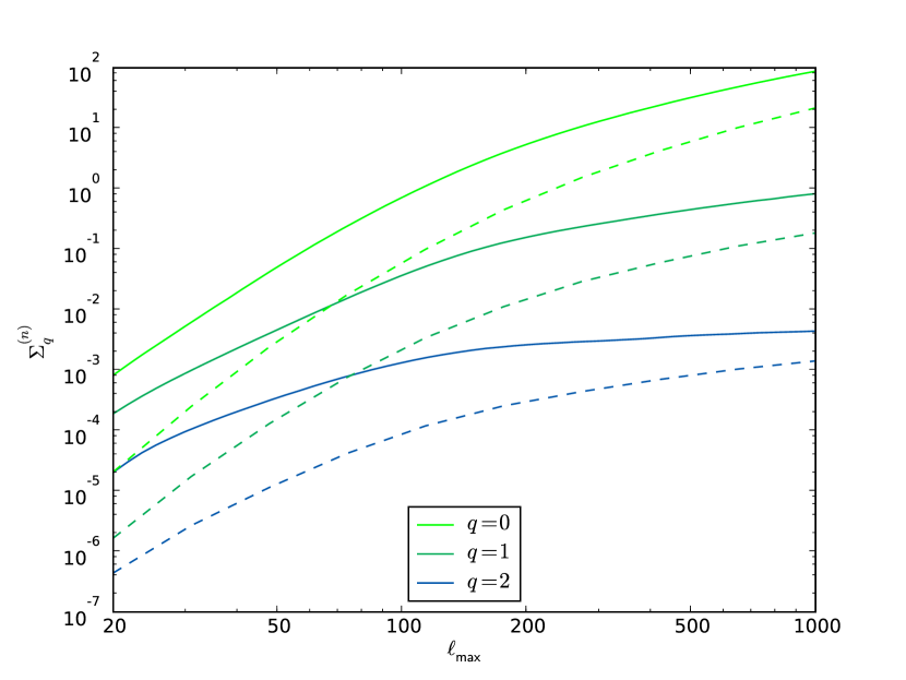
Refer to caption
Figure 8: Cumulative signal-to-noise ratios Σq(n)superscriptsubscriptΣ𝑞𝑛\Sigma_{q}^{(n)} for measurements of the bispectra τqγ3qdelimited-⟨⟩superscript𝜏𝑞superscript𝛾3𝑞\langle\tau^{q}\gamma^{3-q}\rangle (solid lines) and the trispectra τqγ4qdelimited-⟨⟩superscript𝜏𝑞superscript𝛾4𝑞\langle\tau^{q}\gamma^{4-q}\rangle (dashed lines), q=0,1𝑞01q=0,1, for Planck CMB data in cross-correlation with Euclid-like survey, up to a resolution limit max=103subscriptmaxsuperscript103\ell_{\mathrm{max}}=10^{3} starting from a minimum angular wave number of min=10subscriptmin10\ell_{\mathrm{min}}=10.
q𝑞q 00 111 222
Σq(3)superscriptsubscriptΣ𝑞3\Sigma_{q}^{(3)} 87.887.887.8 0.8280.8280.828 4.431034.43superscript1034.43\cdot 10^{-3}
Σq(4)superscriptsubscriptΣ𝑞4\Sigma_{q}^{(4)} 21.721.721.7 0.190.190.19 1.421031.42superscript1031.42\cdot 10^{-3}
Table 2: Cumulative signal-to-noise ratios Σq(n)superscriptsubscriptΣ𝑞𝑛\Sigma_{q}^{(n)} for measurements of the bispectra τqγ3qdelimited-⟨⟩superscript𝜏𝑞superscript𝛾3𝑞\langle\tau^{q}\gamma^{3-q}\rangle and the trispectra τqγ4qdelimited-⟨⟩superscript𝜏𝑞superscript𝛾4𝑞\langle\tau^{q}\gamma^{4-q}\rangle, q=0,1,2𝑞012q=0,1,2, for Planck CMB data in cross-correlation with Euclid-like survey, up to a resolution limit max=103subscriptmaxsuperscript103\ell_{\mathrm{max}}=10^{3} starting from a minimum angular wave number of min=10subscriptmin10\ell_{\mathrm{min}}=10.

The cumulative signal-to-noise ratios Σq(n)superscriptsubscriptΣ𝑞𝑛\Sigma_{q}^{(n)} for the mixed bispectra Bqsubscript𝐵𝑞B_{q} and the mixed trispectra Tqsubscript𝑇𝑞T_{q} are depicted in Fig. 8 for the pure galaxy spectra and spectra with up to two iSW source fields included, q=0,1,2𝑞012q=0,1,2.

The qualitative behavior of the cumulative signal-to-noise curves are again determined by the individual signal strengths of the two source fields γ𝛾\gamma and τ𝜏\tau. The strong fluctuation of the galaxy distribution γ𝛾\gamma even on small scales leads to a considerable increase of ΣΣ\Sigma for large \ell and small q𝑞q. In contrast to this the iSW-effect is a large scale effect and therefore increases the slope in the small \ell limit of the spectrum. It does not contribute significant signal strength above values of max>300subscriptmax300\ell_{\mathrm{max}}>300, for this reason the signal-to-noise curves flatten off in this region of the spectrum for q=1,2𝑞12q=1,2. The wider spread between different values of q𝑞q for the trispectrum in contrast to the bispectrum is due to the higher power of source fields.

Quantitatively, higher values of q𝑞q lead to smaller significance in the signal. Included were contributions starting from large angular scales min=10subscriptmin10\ell_{\mathrm{min}}=10 up to smallest scales measurable in the Planck survey max=103subscriptmaxsuperscript103\ell_{\mathrm{max}}=10^{3}. The pure galaxy polyspectra γ3delimited-⟨⟩superscript𝛾3\langle\gamma^{3}\rangle and γ4delimited-⟨⟩superscript𝛾4\langle\gamma^{4}\rangle can both be measured with a detection significance of 3σmuch-greater-thanabsent3𝜎\gg 3\sigma, Σ0(3)=87.8superscriptsubscriptΣ0387.8\Sigma_{0}^{(3)}=87.8 and Σ0(4)=21.7superscriptsubscriptΣ0421.7\Sigma_{0}^{(4)}=21.7. Including only one iSW source field reduces the signal down to the noise level. While the bispectrum τγ2delimited-⟨⟩𝜏superscript𝛾2\langle\tau\gamma^{2}\rangle reaches a signal-to-noise ratio of 0.820.820.82, the value for the trispectrum τγ3delimited-⟨⟩𝜏superscript𝛾3\langle\tau\gamma^{3}\rangle reaches a maximum of 0.190.190.19. Combining measurements of the q=1𝑞1q=1 bi- and trispectra would therefore be able to contribute a maximum signal-to-noise contribution of Σ0.84Σ0.84\Sigma\approx 0.84. Unfortunately, this is - taken on its own - still a very poor measurement significance. However, it could be used as an additional signal source to the strongest iSW signal from the cross spectrum τγdelimited-⟨⟩𝜏𝛾\langle\tau\gamma\rangle.

For the higher values of q𝑞q only the case of two iSW source fields q=2𝑞2q=2 is plotted in Fig. 8. Both for the bispectrum as well as for the trispectra the signal-to-noise ratios are negligible with maximum values of 4.431034.43superscript1034.43\cdot 10^{-3} and 1.421031.42superscript1031.42\cdot 10^{-3} respectively.

One can obtain a grasp of the differential contributions of the signal-to-noise ratios with respect to angular scale \ell, if one studies the quantity

(ddΣq,equi(3))12superscriptddsuperscriptsubscriptΣ𝑞equi312\displaystyle\left(\frac{\mathrm{d}}{\mathrm{d}\ell}\,\Sigma_{q,\mathrm{equi}}^{(3)}\right)^{\frac{1}{2}} proportional-to\displaystyle\propto Bq,,Cov1(Bq,,)superscriptsubscript𝐵𝑞superscriptCov1superscriptsubscript𝐵𝑞\displaystyle B_{q}^{\ell,\ell,\ell}\sqrt{\mathrm{Cov}^{-1}\left(B_{q}^{\ell,\ell,\ell}\right)}
(ddΣq,square(4))12superscriptddsuperscriptsubscriptΣ𝑞square412\displaystyle\left(\frac{\mathrm{d}}{\mathrm{d}\ell}\,\Sigma_{q,\mathrm{square}}^{(4)}\right)^{\frac{1}{2}} proportional-to\displaystyle\propto Tq,,,,2Cov1(Tq,,,,2).superscriptsubscript𝑇𝑞2superscriptCov1superscriptsubscript𝑇𝑞2\displaystyle T_{q}^{\ell,\ell,\ell,\ell,\sqrt{2}\ell}\sqrt{\mathrm{Cov}^{-1}\left(T_{q}^{\ell,\ell,\ell,\ell,\sqrt{2}\ell}\right)}\,. (65)
Refer to caption
Figure 9: The differential contributions of the equilateral bispectra to the signal-to-noise ratios in dependence on angular wave number \ell are depicted here for different source field mixtures q=0,1,2𝑞012q=0,1,2 (solid lines). For q=1,2𝑞12q=1,2 the contributions from cross-correlations are also shown (dotted lines), as they appear for q=1𝑞1q=1 in the second term of the second line in eqn. (4.3). One can observe the increasing amplitude of the baryonic acoustic oscillations for larger q𝑞q. Also the change in sign can be studied due to the transition from linear dominated to non-linear dominated scales.

In Fig. 9 this differential contribution of equilateral bispectra in dependence on \ell are depicted for different source field mixtures q𝑞q. The differential contributions of the square trispectra behave qualitatively analogous. Also the change in sign can be studied due to the transition from linear dominated to non-linear dominated scales. For q=1,2𝑞12q=1,2 the contributions from cross-correlations are also shown (dotted lines), as they appear for q=1𝑞1q=1 in the second term of the second line in eqn. (4.3). As one can see, these terms are subdominant and can be neglected in our case.

One can observe the increasing amplitude of the baryonic acoustic oscillations for larger q𝑞q, which originate from CCMBsuperscriptsubscript𝐶CMBC_{\mathrm{CMB}}^{\ell}. The falling slopes of the BAO features in the covariance lead to small plateaus in the differential contributions for larger \ell. Since in these regions the signal decreases more gently than the covariance, one obtains a local increase of signal-to-noise. However, this effect can hardly be observed in Fig. 8.

5 SUMMARY

The objective of this work is a study of the detectability of non-Gaussian signatures in non-linear iSW-effect. Besides the mixed bispectra of the form τqγ3qdelimited-⟨⟩superscript𝜏𝑞superscript𝛾3𝑞\langle\tau^{q}\gamma^{3-q}\rangle, q=0,1,2𝑞012q=0,1,2, between the galaxy distribution γ𝛾\gamma and the iSW temperature perturbation τ𝜏\tau we also calculate for the first time the mixed trispectra of the analogous form τqγ4qdelimited-⟨⟩superscript𝜏𝑞superscript𝛾4𝑞\langle\tau^{q}\gamma^{4-q}\rangle. Both types of spectra were consistently derived in tree-level perturbation theory in Newtonian gravity. This implies for the bispectra perturbative corrections to second order and for the mixed trispectra contributions from second and third order terms. Furthermore, we investigated the time evolution of these individual 3-dimensional source terms, which are in general very diverse. For this reason, the time evolution and the configuration dependence of a specific class of spectra, equilateral bispectra and the square trispectra, were studied. Finally, the achievable signal-to-noise ratios were derived for measurements cross-correlating Planck data and a galaxy sample, as it would be expected from a wide angle survey as Euclid.

(i) The linear iSW-effect has the time dependence d(D+/a)/dadsubscript𝐷𝑎d𝑎\mathrm{d}(D_{+}/a)/\mathrm{d}a, which makes it sensitive to dark energy but vanishes in SCDM-models with Ωm1subscriptΩm1\Omega_{\mathrm{m}}\equiv 1 and D+(a)=asubscript𝐷𝑎𝑎D_{+}(a)=a. In contrast to this, the non-linear contributions to the iSW signal are sensitive to derivatives of higher powers of D+(a)subscript𝐷𝑎D_{+}(a), namely d(D+2/a)/dadsuperscriptsubscript𝐷2𝑎d𝑎\mathrm{d}(D_{+}^{2}/a)/\mathrm{d}a for second order perturbation theory and d(D+3/a)/dadsuperscriptsubscript𝐷3𝑎d𝑎\mathrm{d}(D_{+}^{3}/a)/\mathrm{d}a for third order contributions. For this reason, the effect does not vanish in matter-dominated epochs.

(ii) The covariances of the measurements were derived in a Gaussian approximation. For the CMB observation the intrinsic CMB fluctuations and instrumental noise in form of the pixel noise and a Gaussian beam were considered as noise sources. A Poissonian noise term was added to the galaxy distribution signal. For simplicity the fluctuations of the dark matter density and galaxy number density were related to each other by a constant linear biasing model.

(iii) In the mixed bispectra and trispectra the configuration and scale dependence represent the different correlation lengths of the gravitational potential and the density field. Since the specific perturbative corrections dominate on different scales, the mixed spectra change their sign at certain values of \ell. In case of the bispectra one can observe the transition from linear domination to non-linear domination move to larger and larger scales with increasing number of included iSW source fields q𝑞q.

(iv) We derived the cumulative signal-to-noise ratios Σq(3)superscriptsubscriptΣ𝑞3\Sigma_{q}^{(3)} for the measurements of mixed bispectra τqγ3qdelimited-⟨⟩superscript𝜏𝑞superscript𝛾3𝑞\langle\tau^{q}\gamma^{3-q}\rangle, and Σq(4)superscriptsubscriptΣ𝑞4\Sigma_{q}^{(4)} for the mixed trispectra of the form τqγ4qdelimited-⟨⟩superscript𝜏𝑞superscript𝛾4𝑞\langle\tau^{q}\gamma^{4-q}\rangle, with a Gaussian approximation to the covariance. The integration were performed numerically using Monte Carlo integration techniques from the multidimensional numerical integration library CUBA (Hahn 2005). For both spectra the initial CMB fluctuations are the most important noise source, which makes it difficult to observe the signals. We assumed a cross-correlation of Planck data with a Euclid-like galaxy sample starting from angular scales of min=10subscriptmin10\ell_{\mathrm{min}}=10 up to a resolution of max=103subscriptmaxsuperscript103\ell_{\mathrm{max}}=10^{3}. The only spectra reaching the order of magnitude of the noise level are the bispectra and trispectra in the configuration τγn1delimited-⟨⟩𝜏superscript𝛾𝑛1\langle\tau\gamma^{n-1}\rangle. We found the numerical signal-to-noise ratios of Σ1(3)=0.828superscriptsubscriptΣ130.828\Sigma_{1}^{(3)}=0.828 for the bispectrum and Σ1(4)=0.19superscriptsubscriptΣ140.19\Sigma_{1}^{(4)}=0.19 for the trispectrum and conclude, that non-Gaussian signatures of the iSW-effect are too weak to be detected. At the same time, these small signal-to-noise ratios suggest that non-Gaussianities in the CMB generated by the iSW-effect are small enough so that they do not interfere with the estimation of the inflationary non-Gaussianity parameter fNLsubscript𝑓NLf_{\mathrm{NL}} from the bispectrum τ3delimited-⟨⟩superscript𝜏3\langle\tau^{3}\rangle and of the two parameters gNLsubscript𝑔NLg_{\mathrm{NL}} and τNLsubscript𝜏NL\tau_{\mathrm{NL}} from the trispectrum τ4delimited-⟨⟩superscript𝜏4\langle\tau^{4}\rangle.

ACKNOWLEDGEMENTS

We would like to thank Matthias Bartelmann for useful discussions and ideas. Our work was supported by the German Research Foundation (DFG) within the framework of the Priority Programme 1177 and the excellence initiative through the Heidelberg Graduate School of Fundamental Physics.

References

  • Abramowitz & Stegun (1972) Abramowitz M., Stegun I. A., 1972, Handbook of Mathematical Functions
  • Aghanim et al. (2008) Aghanim N., Majumdar S., Silk J., 2008, Reports on Progress in Physics, 71, 066902
  • Bardeen et al. (1986) Bardeen J. M., Bond J. R., Kaiser N., Szalay A. S., 1986, ApJ, 304, 15
  • Bernardeau et al. (2002) Bernardeau F., Colombi S., Gaztañaga E., Scoccimarro R., 2002, Physics Reports, 367, 1
  • Boughn & Crittenden (2004) Boughn S., Crittenden R., 2004, Nature, 427, 45
  • Boughn et al. (1998) Boughn S. P., Crittenden R. G., Turok N. G., 1998, New Astronomy, 3, 275
  • Cooray (2002) Cooray A., 2002, Phys. Rev. D, 65, 083518
  • Crittenden & Turok (1996) Crittenden R. G., Turok N., 1996, Physical Review Letters, 76, 575
  • Fixsen (2009) Fixsen D. J., 2009, ApJ, 707, 916
  • Giannantonio et al. (2008) Giannantonio T., Scranton R., Crittenden R. G., Nichol R. C., Boughn S. P., Myers A. D., Richards G. T., 2008, Phys. Rev. D, 77, 123520
  • Goroff et al. (1986) Goroff M. H., Grinstein B., Rey S.-J., Wise M. B., 1986, ApJ, 311, 6
  • Hahn (2005) Hahn T., 2005, Computer Physics Communications, 168, 78
  • Hernández-Monteagudo (2010) Hernández-Monteagudo C., 2010, A&A, 520, A101
  • Hu (2000) Hu W., 2000, Phys. Rev. D, 62, 043007
  • Hu (2001) Hu W., 2001, Phys. Rev. D, 64, 083005
  • Jain & Bertschinger (1994) Jain B., Bertschinger E., 1994, ApJ, 431, 495
  • Lewis et al. (2000) Lewis A., Challinor A., Lasenby A., 2000, ApJ, 538, 473
  • Limber (1953) Limber D. N., 1953, ApJ, 117, 134
  • Linder & Jenkins (2003) Linder E. V., Jenkins A., 2003, MNRAS, 346, 573
  • López-Corredoira et al. (2010) López-Corredoira M., Sylos Labini F., Betancort-Rijo J., 2010, A&A, 513, A3
  • Lue et al. (2004) Lue A., Scoccimarro R., Starkman G., 2004, Phys. Rev. D, 69, 044005
  • Martinez-Gonzalez et al. (1994) Martinez-Gonzalez E., Sanz J. L., Silk J., 1994, ApJ, 436, 1
  • McEwen et al. (2007) McEwen J. D., Vielva P., Hobson M. P., Martínez-González E., Lasenby A. N., 2007, MNRAS, 376, 1211
  • Mo et al. (1997) Mo H. J., Jing Y. P., White S. D. M., 1997, MNRAS, 284, 189
  • Nishizawa et al. (2008) Nishizawa A. J., Komatsu E., Yoshida N., Takahashi R., Sugiyama N., 2008, ApJL, 676, L93
  • Ostriker & Vishniac (1986) Ostriker J. P., Vishniac E. T., 1986, ApJL, 306, L51
  • Rees & Sciama (1968) Rees M. J., Sciama D. W., 1968, Nature, 217, 511
  • Sachs & Wolfe (1967) Sachs R. K., Wolfe A. M., 1967, ApJ, 147, 73
  • Sahni & Coles (1995) Sahni V., Coles P., 1995, Physics Reports, 262, 1
  • Sanz et al. (1996) Sanz J. L., Martinez-Gonzalez E., Cayon L., Silk J., Sugiyama N., 1996, ApJ, 467, 485
  • Schäfer (2008) Schäfer B. M., 2008, MNRAS, 388, 1394
  • Schäfer & Bartelmann (2006) Schäfer B. M., Bartelmann M., 2006, MNRAS, 369, 425
  • Seljak (1996) Seljak U., 1996, ApJ, 460, 549
  • Sheth et al. (2001) Sheth R. K., Mo H. J., Tormen G., 2001, MNRAS, 323, 1
  • Smail et al. (1995) Smail I., Hogg D. W., Blandford R., Cohen J. G., Edge A. C., Djorgovski S. G., 1995, MNRAS, 277, 1
  • Spergel et al. (2003) Spergel D. N., Verde L., Peiris H. V., Komatsu E., Nolta M. R., Bennett C. L., Halpern M., Hinshaw G., Jarosik N., Kogut A., Limon M., Meyer S. S., Page L., Tucker G. S., Weiland J. L., Wollack E., Wright E. L., 2003, ApJS, 148, 175
  • Sugiyama (1995) Sugiyama N., 1995, ApJS, 100, 281
  • Tuluie & Laguna (1995) Tuluie R., Laguna P., 1995, ApJL, 445, L73
  • Turner & White (1997) Turner M. S., White M., 1997, Phys. Rev. D, 56, 4439
  • Vielva et al. (2006) Vielva P., Martínez-González E., Tucci M., 2006, MNRAS, 365, 891
  • Wang & Steinhardt (1998) Wang L., Steinhardt P. J., 1998, ApJ, 508, 483
  • Zaldarriaga et al. (1997) Zaldarriaga M., Spergel D. N., Seljak U., 1997, ApJ, 488, 1
  • Zeldovich & Sunyaev (1980) Zeldovich Y. B., Sunyaev S. R. A., 1980, Pis ma Astronomicheskii Zhurnal, 6, 737
  • Zhang (2006) Zhang P., 2006, Phys. Rev. D, 73, 123504

Appendix A Analytical details of signal-to-noise ratios

The squared signal-to-noise ratio Σ2superscriptΣ2\Sigma^{2} is given by the χ2superscript𝜒2\chi^{2} between a detection and its zero hypothesis. In the course of its calculation, one has to ensure that no redundant information is taken into account. We present the calculation for the bispectra only, since it follows the same argumentation in the case of the trispectra. Neglecting redundancy due to any symmetries all mixed and pure bispectra would account for a χ2superscript𝜒2\chi^{2}- contribution of

χ2superscript𝜒2\displaystyle\chi^{2} =\displaystyle= fskyπ1(2π)2d21,2,3d21,2,3δD(1+2+3)subscript𝑓sky𝜋1superscript2𝜋2superscriptd2subscriptbold-ℓ123superscriptd2subscriptbold-ℓsuperscript1superscript2superscript3subscript𝛿Dsubscriptbold-ℓ1subscriptbold-ℓ2subscriptbold-ℓ3\displaystyle\frac{f_{\mathrm{sky}}}{\pi}\frac{1}{(2\pi)^{2}}\int\mathrm{d}^{2}\mn@boldsymbol{\ell}_{1,2,3}\,\mathrm{d}^{2}\mn@boldsymbol{\ell}_{1^{\prime},2^{\prime},3^{\prime}}\,\,\delta_{\mathrm{D}}(\mn@boldsymbol{\ell}_{1}+\mn@boldsymbol{\ell}_{2}+\mn@boldsymbol{\ell}_{3})
Bi1i2i31,2,3Cov1[B~i1i2i31,2,3,B~i1i2i31,2,3]B~i1i2i31,2,3,superscriptsubscript𝐵subscript𝑖1subscript𝑖2subscript𝑖3subscript1subscript2subscript3superscriptCov1superscriptsubscript~𝐵subscript𝑖1subscript𝑖2subscript𝑖3subscript1subscript2subscript3superscriptsubscript~𝐵superscriptsubscript𝑖1superscriptsubscript𝑖2superscriptsubscript𝑖3superscriptsubscript1superscriptsubscript2superscriptsubscript3superscriptsubscript~𝐵superscriptsubscript𝑖1superscriptsubscript𝑖2superscriptsubscript𝑖3superscriptsubscript1superscriptsubscript2superscriptsubscript3\displaystyle B_{i_{1}i_{2}i_{3}}^{\,\ell_{1},\ell_{2},\ell_{3}}\,\mathrm{Cov}^{-1}\left[\tilde{B}_{i_{1}i_{2}i_{3}}^{\,\ell_{1},\ell_{2},\ell_{3}},\tilde{B}_{i_{1}^{\prime}i_{2}^{\prime}i_{3}^{\prime}}^{\,\ell_{1}^{\prime},\ell_{2}^{\prime},\ell_{3}^{\prime}}\right]\,\tilde{B}_{i_{1}^{\prime}i_{2}^{\prime}i_{3}^{\prime}}^{\,\ell_{1}^{\prime},\ell_{2}^{\prime},\ell_{3}^{\prime}}\,, (66)

where also the sum over all field indices is implied. However, the integrand is symmetric in any simultaneous pairwise permutation of (n,in)subscriptbold-ℓ𝑛subscript𝑖𝑛(\mn@boldsymbol{\ell}_{n},i_{n}) with (m,im)subscriptbold-ℓ𝑚subscript𝑖𝑚(\mn@boldsymbol{\ell}_{m},i_{m}) and likewise of (n,in)superscriptsubscriptbold-ℓ𝑛superscriptsubscript𝑖𝑛(\mn@boldsymbol{\ell}_{n}^{\prime},i_{n}^{\prime}) with (m,im)superscriptsubscriptbold-ℓ𝑚superscriptsubscript𝑖𝑚(\mn@boldsymbol{\ell}_{m}^{\prime},i_{m}^{\prime}). This type of redundancy can be avoided by constraining the integration volumes to 1<2<3subscript1subscript2subscript3\ell_{1}<\ell_{2}<\ell_{3} and 1<2<3superscriptsubscript1superscriptsubscript2superscriptsubscript3\ell_{1}^{\prime}<\ell_{2}^{\prime}<\ell_{3}^{\prime}. Furthermore, the sum over field indices may lead to more redundancy, which we encode at this point into a multiplicity factor si1i2i3i1i2i3superscriptsubscript𝑠subscript𝑖1subscript𝑖2subscript𝑖3superscriptsubscript𝑖1superscriptsubscript𝑖2superscriptsubscript𝑖3s_{i_{1}i_{2}i_{3}}^{i_{1}^{\prime}i_{2}^{\prime}i_{3}^{\prime}}. Now, the signal-to-noise ratio can be written as

(Σ(3))2=fsky4π31<2<3d21,2,31<2<3d21,2,3δD(1+2+3)×Bi1i2i31,2,3Cov1[B~i1i2i31,2,3,B~i1i2i31,2,3]B~i1i2i31,2,3(si1i2i3i1i2i3)1,superscriptsuperscriptΣ32subscript𝑓sky4superscript𝜋3subscriptsubscript1subscript2subscript3superscriptd2subscriptbold-ℓ123subscriptsuperscriptsubscript1superscriptsubscript2superscriptsubscript3superscriptd2subscriptbold-ℓsuperscript1superscript2superscript3subscript𝛿Dsubscriptbold-ℓ1subscriptbold-ℓ2subscriptbold-ℓ3superscriptsubscript𝐵subscript𝑖1subscript𝑖2subscript𝑖3subscript1subscript2subscript3superscriptCov1superscriptsubscript~𝐵subscript𝑖1subscript𝑖2subscript𝑖3subscript1subscript2subscript3superscriptsubscript~𝐵superscriptsubscript𝑖1superscriptsubscript𝑖2superscriptsubscript𝑖3superscriptsubscript1superscriptsubscript2superscriptsubscript3superscriptsubscript~𝐵superscriptsubscript𝑖1superscriptsubscript𝑖2superscriptsubscript𝑖3superscriptsubscript1superscriptsubscript2superscriptsubscript3superscriptsuperscriptsubscript𝑠subscript𝑖1subscript𝑖2subscript𝑖3superscriptsubscript𝑖1superscriptsubscript𝑖2superscriptsubscript𝑖31\left(\Sigma^{(3)}\right)^{2}=\frac{f_{\mathrm{sky}}}{4\pi^{3}}\int\limits_{\ell_{1}<\ell_{2}<\ell_{3}}\mathrm{d}^{2}\mn@boldsymbol{\ell}_{1,2,3}\,\int\limits_{\ell_{1}^{\prime}<\ell_{2}^{\prime}<\ell_{3}^{\prime}}\mathrm{d}^{2}\mn@boldsymbol{\ell}_{1^{\prime},2^{\prime},3^{\prime}}\,\,\delta_{\mathrm{D}}(\mn@boldsymbol{\ell}_{1}+\mn@boldsymbol{\ell}_{2}+\mn@boldsymbol{\ell}_{3})\\ \times B_{i_{1}i_{2}i_{3}}^{\,\ell_{1},\ell_{2},\ell_{3}}\,\mathrm{Cov}^{-1}\left[\tilde{B}_{i_{1}i_{2}i_{3}}^{\,\ell_{1},\ell_{2},\ell_{3}},\tilde{B}_{i_{1}^{\prime}i_{2}^{\prime}i_{3}^{\prime}}^{\,\ell_{1}^{\prime},\ell_{2}^{\prime},\ell_{3}^{\prime}}\right]\,\tilde{B}_{i_{1}^{\prime}i_{2}^{\prime}i_{3}^{\prime}}^{\,\ell_{1}^{\prime},\ell_{2}^{\prime},\ell_{3}^{\prime}}\,\left(s_{i_{1}i_{2}i_{3}}^{i_{1}^{\prime}i_{2}^{\prime}i_{3}^{\prime}}\right)^{-1}\,, (67)

In this subspace the covariance matrix can be inverted, as it was shown in Section 4.2. Substituting eqn. (60) into eqn. (67), we find

(Σ(3))2=fsky4π3(si1i2i3i1i2i3)11<2<3d21d22×Bi1i2i31,2,3C~i1i11C~i2i22C~i3i33detC1detC2detC3B~i1i2i31,2,3,superscriptsuperscriptΣ32subscript𝑓sky4superscript𝜋3superscriptsuperscriptsubscript𝑠subscript𝑖1subscript𝑖2subscript𝑖3superscriptsubscript𝑖1superscriptsubscript𝑖2superscriptsubscript𝑖31subscriptsubscript1subscript2subscript3superscriptd2subscriptbold-ℓ1superscriptd2subscriptbold-ℓ2superscriptsubscript𝐵subscript𝑖1subscript𝑖2subscript𝑖3subscript1subscript2subscript3superscriptsubscript~𝐶superscriptsubscript𝑖1absentsuperscriptsubscript𝑖1absentsubscript1superscriptsubscript~𝐶superscriptsubscript𝑖2absentsuperscriptsubscript𝑖2absentsubscript2superscriptsubscript~𝐶superscriptsubscript𝑖3absentsuperscriptsubscript𝑖3absentsubscript3superscript𝐶subscript1superscript𝐶subscript2superscript𝐶subscript3superscriptsubscript~𝐵superscriptsubscript𝑖1superscriptsubscript𝑖2superscriptsubscript𝑖3subscript1subscript2subscript3\left(\Sigma^{(3)}\right)^{2}=\frac{f_{\mathrm{sky}}}{4\pi^{3}}\,\left(s_{i_{1}i_{2}i_{3}}^{i_{1}^{\prime}i_{2}^{\prime}i_{3}^{\prime}}\right)^{-1}\int\limits_{\ell_{1}<\ell_{2}<\ell_{3}}\mathrm{d}^{2}\mn@boldsymbol{\ell}_{1}\,\mathrm{d}^{2}\mn@boldsymbol{\ell}_{2}\,\\ \times B_{i_{1}i_{2}i_{3}}^{\,\ell_{1},\ell_{2},\ell_{3}}\,\frac{\tilde{C}_{i_{1}^{~{}}i_{1}^{\prime}}^{\ast\,\ell_{1}}\tilde{C}_{i_{2}^{~{}}i_{2}^{\prime}}^{\ast\,\ell_{2}}\tilde{C}_{i_{3}^{~{}}i_{3}^{\prime}}^{\ast\,\ell_{3}}}{\det C^{\,\ell_{1}}\det C^{\,\ell_{2}}\det C^{\,\ell_{3}}}\tilde{B}_{i_{1}^{\prime}i_{2}^{\prime}i_{3}^{\prime}}^{\,\ell_{1},\ell_{2},\ell_{3}}\,, (68)

where from now on 3=12subscriptbold-ℓ3subscriptbold-ℓ1subscriptbold-ℓ2\mn@boldsymbol{\ell}_{3}=-\mn@boldsymbol{\ell}_{1}-\mn@boldsymbol{\ell}_{2} is implied, if 3subscriptbold-ℓ3\mn@boldsymbol{\ell}_{3} is not integrated over. If one is now interested in the signal-to-noise ratio of particular field mixture, i.e. data with a fixed field configuration q=i1+i2+i3𝑞subscript𝑖1subscript𝑖2subscript𝑖3q=i_{1}+i_{2}+i_{3}, one can further simplify the expression. For pure galaxy contributions, q=q=0𝑞superscript𝑞0q=q^{\prime}=0, we can neglect the cross-correlation , i.e. C01=0subscript𝐶010C_{01}=0, and no redundancy due to field summation occurs, s000000=1superscriptsubscript𝑠0000001s_{000}^{000}=1. One obtains the well-known case (Hu, 2001)

(Σ0(3))2=fsky4π3d21d22(B0001,2,3)26C~001C~002C~003,superscriptsuperscriptsubscriptΣ032subscript𝑓sky4superscript𝜋3superscriptd2subscriptbold-ℓ1superscriptd2subscriptbold-ℓ2superscriptsuperscriptsubscript𝐵000subscript1subscript2subscript326superscriptsubscript~𝐶00subscript1superscriptsubscript~𝐶00subscript2superscriptsubscript~𝐶00subscript3\left(\Sigma_{0}^{(3)}\right)^{2}=\frac{f_{\mathrm{sky}}}{4\pi^{3}}\,\int\mathrm{d}^{2}\mn@boldsymbol{\ell}_{1}\,\mathrm{d}^{2}\mn@boldsymbol{\ell}_{2}\,\frac{\left(B_{000}^{\,\ell_{1},\ell_{2},\ell_{3}}\right)^{2}}{6\,\tilde{C}_{00}^{\,\ell_{1}}\tilde{C}_{00}^{\,\ell_{2}}\tilde{C}_{00}^{\,\ell_{3}}}\,, (69)

where the symmetry in the integrand was used to obtain an integration over full bold-ℓ\mn@boldsymbol{\ell}-space in combination with the factor 1/6161/6. If all mixed spectra with one iSW field are taken into account, i.e. q=q=1𝑞superscript𝑞1q=q^{\prime}=1, one obtains 999 different contributions due to the field index summation. Three contributions are quadratic in identical bispectra, (i1,i2,i3)=(i1,i2,i3)subscript𝑖1subscript𝑖2subscript𝑖3superscriptsubscript𝑖1superscriptsubscript𝑖2superscriptsubscript𝑖3(i_{1},i_{2},i_{3})=(i_{1}^{\prime},i_{2}^{\prime},i_{3}^{\prime}), and have multiplicity one. The remaining mixed contributions have multiplicity 2, since the integrand in eqn. (68) is symmetric under exchange of the primed and unprimed index sets (i1,i2,i3)subscript𝑖1subscript𝑖2subscript𝑖3(i_{1},i_{2},i_{3}) and (i1,i2,i3)superscriptsubscript𝑖1superscriptsubscript𝑖2superscriptsubscript𝑖3(i_{1}^{\prime},i_{2}^{\prime},i_{3}^{\prime}) as a whole. Therefore the multiplicities are

11\displaystyle 1 =\displaystyle= s001001=s010010=s100100superscriptsubscript𝑠001001superscriptsubscript𝑠010010superscriptsubscript𝑠100100\displaystyle s_{001}^{001}=s_{010}^{010}=s_{100}^{100}
22\displaystyle 2 =\displaystyle= s001010=s001100=s010100=s010001=s100001=s100010.superscriptsubscript𝑠001010superscriptsubscript𝑠001100superscriptsubscript𝑠010100superscriptsubscript𝑠010001superscriptsubscript𝑠100001superscriptsubscript𝑠100010\displaystyle s_{001}^{010}=s_{001}^{100}=s_{010}^{100}=s_{010}^{001}=s_{100}^{001}=s_{100}^{010}\,. (70)

If one uses

B0101,2,3superscriptsubscript𝐵010subscript1subscript2subscript3\displaystyle B_{010}^{\,\ell_{1},\ell_{2},\ell_{3}} =\displaystyle= B0011,3,2superscriptsubscript𝐵001subscript1subscript3subscript2\displaystyle B_{001}^{\,\ell_{1},\ell_{3},\ell_{2}}
B1001,2,3superscriptsubscript𝐵100subscript1subscript2subscript3\displaystyle B_{100}^{\,\ell_{1},\ell_{2},\ell_{3}} =\displaystyle= B0013,2,1superscriptsubscript𝐵001subscript3subscript2subscript1\displaystyle B_{001}^{\,\ell_{3},\ell_{2},\ell_{1}} (71)

in combination with

B0011,2,3superscriptsubscript𝐵001subscript1subscript2subscript3\displaystyle B_{001}^{\,\ell_{1},\ell_{2},\ell_{3}} =\displaystyle= 12(B0011,2,3+B0012,1,3),12superscriptsubscript𝐵001subscript1subscript2subscript3superscriptsubscript𝐵001subscript2subscript1subscript3\displaystyle\frac{1}{2}\left(B_{001}^{\,\ell_{1},\ell_{2},\ell_{3}}+B_{001}^{\,\ell_{2},\ell_{1},\ell_{3}}\right)\,, (72)

one can combine the quadratic terms to one, which is integrated over the full 1,2,3subscriptbold-ℓ123\mn@boldsymbol{\ell}_{1,2,3}-volume. This can be done for the mixed terms in analogy and one is left with the following expression for the signal-to-noise ratio,

(Σ1(3))2=fsky4π3d21d22(2detC1detC2detC3)1[(B0011,2,3)2C~111C~112C~003+B0011,2,3C~111C~012C~013B0101,2,3].superscriptsuperscriptsubscriptΣ132subscript𝑓sky4superscript𝜋3superscriptd2subscriptbold-ℓ1superscriptd2subscriptbold-ℓ2superscript2superscript𝐶subscript1superscript𝐶subscript2superscript𝐶subscript31delimited-[]superscriptsuperscriptsubscript𝐵001subscript1subscript2subscript32superscriptsubscript~𝐶11subscript1superscriptsubscript~𝐶11subscript2superscriptsubscript~𝐶00subscript3superscriptsubscript𝐵001subscript1subscript2subscript3superscriptsubscript~𝐶11subscript1superscriptsubscript~𝐶01subscript2superscriptsubscript~𝐶01subscript3superscriptsubscript𝐵010subscript1subscript2subscript3\left(\Sigma_{1}^{(3)}\right)^{2}=\frac{f_{\mathrm{sky}}}{4\pi^{3}}\int\mathrm{d}^{2}\mn@boldsymbol{\ell}_{1}\,\mathrm{d}^{2}\mn@boldsymbol{\ell}_{2}\,\,\left(2\,\det C^{\,\ell_{1}}\det C^{\,\ell_{2}}\det C^{\,\ell_{3}}\right)^{-1}\\ \left[\left(B_{001}^{\,\ell_{1},\ell_{2},\ell_{3}}\right)^{2}\tilde{C}_{11}^{\,\ell_{1}}\tilde{C}_{11}^{\,\ell_{2}}\tilde{C}_{00}^{\,\ell_{3}}+B_{001}^{\,\ell_{1},\ell_{2},\ell_{3}}\tilde{C}_{11}^{\,\ell_{1}}\tilde{C}_{01}^{\,\ell_{2}}\tilde{C}_{01}^{\,\ell_{3}}B_{010}^{\,\ell_{1},\ell_{2},\ell_{3}}\right]\,. (73)

Following the analog path of argumentation one finds the signal-to-noise expressions for the trispectra to be

(Σ0(4))2superscriptsuperscriptsubscriptΣ042\displaystyle\left(\Sigma_{0}^{(4)}\right)^{2} =\displaystyle= fsky8π4d21d22d23(T00001,2,3,4)224C~001C~002C~003C~004subscript𝑓sky8superscript𝜋4superscriptd2subscriptbold-ℓ1superscriptd2subscriptbold-ℓ2superscriptd2subscriptbold-ℓ3superscriptsuperscriptsubscript𝑇0000subscript1subscript2subscript3subscript4224superscriptsubscript~𝐶00subscript1superscriptsubscript~𝐶00subscript2superscriptsubscript~𝐶00subscript3superscriptsubscript~𝐶00subscript4\displaystyle\frac{f_{\mathrm{sky}}}{8\pi^{4}}\int\mathrm{d}^{2}\mn@boldsymbol{\ell}_{1}\,\mathrm{d}^{2}\mn@boldsymbol{\ell}_{2}\,\mathrm{d}^{2}\mn@boldsymbol{\ell}_{3}\,\,\frac{\left(T_{0000}^{\,\ell_{1},\ell_{2},\ell_{3},\ell_{4}}\right)^{2}}{24\,\tilde{C}_{00}^{\,\ell_{1}}\tilde{C}_{00}^{\,\ell_{2}}\tilde{C}_{00}^{\,\ell_{3}}\tilde{C}_{00}^{\,\ell_{4}}}
(Σ1(4))2superscriptsuperscriptsubscriptΣ142\displaystyle\left(\Sigma_{1}^{(4)}\right)^{2} =\displaystyle= fsky8π4d21d22d23(detC1detC4)1subscript𝑓sky8superscript𝜋4superscriptd2subscriptbold-ℓ1superscriptd2subscriptbold-ℓ2superscriptd2subscriptbold-ℓ3superscriptsuperscript𝐶subscript1superscript𝐶subscript41\displaystyle\frac{f_{\mathrm{sky}}}{8\pi^{4}}\int\mathrm{d}^{2}\mn@boldsymbol{\ell}_{1}\,\mathrm{d}^{2}\mn@boldsymbol{\ell}_{2}\,\mathrm{d}^{2}\mn@boldsymbol{\ell}_{3}\,\,\left(\det C^{\,\ell_{1}}\dots\det C^{\,\ell_{4}}\right)^{-1}
[16(T00011,2,3,4)2C~111C~112C~113C~004\displaystyle\left[\,\,\,\frac{1}{6}\,\left(T_{0001}^{\,\ell_{1},\ell_{2},\ell_{3},\ell_{4}}\right)^{2}\tilde{C}_{11}^{\,\ell_{1}}\tilde{C}_{11}^{\,\ell_{2}}\tilde{C}_{11}^{\,\ell_{3}}\tilde{C}_{00}^{\,\ell_{4}}\right.
+14T00011,2,3,4C~111C~112C~013C~014T00101,2,3,4].\displaystyle+\,\frac{1}{4}\,\left.T_{0001}^{\,\ell_{1},\ell_{2},\ell_{3},\ell_{4}}\tilde{C}_{11}^{\,\ell_{1}}\tilde{C}_{11}^{\,\ell_{2}}\tilde{C}_{01}^{\,\ell_{3}}\tilde{C}_{01}^{\,\ell_{4}}T_{0010}^{\,\ell_{1},\ell_{2},\ell_{3},\ell_{4}}\,\right]\,. (74)

Also the expressions for higher values of q𝑞q can now be deduced with the same techniques.