The role of the disorder range and electronic energy in the graphene nanoribbons perfect transmission

Abstract

Numerical calculations based on the recursive Green’s functions method in the tight-binding approximation are performed to calculate the dimensionless conductance $g$ in disordered graphene nanoribbons with Gaussian scatterers. The influence of the transition from short- to long-ranged disorder on $g$ is studied as well as its effects on the formation of a perfectly conducting channel. We also investigate the dependence of electronic energy on the perfectly conducting channel. We propose and calculate a backscattering estimative in order to establish the connection between the perfectly conducting channel (with $g=1$) and the amount of intervalley scattering.

I Introduction

The remarkable electronic transport properties of graphene have motivated numerous experimental and theoretical studies. Castro Neto et al. (2009); Mucciolo and Lewenkopf (2010); Sarma et al. (2010) Of particular interest is the possibility of fabricating narrow width graphene samples, called graphene nanoribbons (GNRs). By engineering the lateral confinement one can, in principle, create an electronic energy gap leading to a semiconductor behavior that allows for the development of novel electronic nanodevices and applications. Geim (2009)

The observation of conductance quantization in GNRs turned out to be more difficult than anticipated Lin et al. (2008). The reason is that the vast majority of GNR samples are produced by lithographic patterning, characterized by rough edges at the atomic scale Molitor et al. (2009); Stampfer et al. (2009); Han et al. (2010); Todd et al. (2009); Gallagher et al. (2010). Already at low concentrations, such defects can destroy conductance quantization Lewenkopf et al. (2008). Edge roughness may be largely suppressed in GNRs produced by unzipping single-wall carbon nanotube. Li et al. (2008); Jiao et al. (2010, 2011) However, the latter is not free of bulk defects.

The way disorder affects electronic transport in GNRs strongly depends on its spatial range. For long-ranged disorder (LRD), corresponding to a ratio $d/a_{0}\gg 1$ between the potential range $d$ and the lattice parameter $a_{0}$, backscattering is suppressed and the transmission is little affected. In contrast, short-ranged disorder (SRD) favors scattering processes with large momentum transfer such as backscattering. In this regime, quantum interference can cause wave function localization. In general, these simple arguments provide a qualitative explanation for the observed behavior of the conductance in current experiments. Edge roughness is essentially short ranged, while substrate impurity charges and ionically bonded adatoms are the typical sources of long-ranged disorder. Lewenkopf et al. (2008)

In view of the unavoidable disorder, the natural question that arises is whether one can indeed observe perfect transmission or conductance quantization in GNRs. This question has been theoretically investigated and partially answered by Wakabayashi et al. Wakabayashi et al. (2007, 2009). They have found that zigzag edge GNRs in the presence of long-range disorder exhibits a quite robust perfectly conducting channel (PCC).

The dispersion relation for zigzag GNRs, Fig. 1, helps one to understand the origin of PCC. Fig. 1 indicates two possible transversal momentum states for electronic energies such that, at low enough energies, only the first sub-band is allowed. The state close to the $K$ point corresponds to a right propagating channel whereas the other, close to $K^{\prime}$, is related to a left propagating channel Wakabayashi et al. (2009). In this case, electrons propagate through the system in a well-defined direction leading to perfect transmission. Disorder can modify this scenario, provided it can cause a momentum transfer $\Delta k\approx|K-K^{\prime}|\approx 1/a_{0}$ so that it mixes left and right propagating channels. In other words, this backscattering process requires a momentum transfer from states at the vicinity of the $K$-point (reminiscent of bulk graphene) to the $K^{\prime}$ point, and vice-versa. The correspondence between short-ranged defects in rough-edged GNRs and intervalley scattering has been established by analyzing the scattering processes in both real and Fourier space Libisch et al. (2011). For LRD such correspondence is more subtle and has been recently addressed by analyzing the reflection probabilities of zigzag and armchair GNRs and their symmetry properties Wurm et al. (2012). For disordered zigzag GNRs, electronic scattering should mix valleys, leading to the suppression of transmission depending on $d$. We address this issue by establishing a connection between the PCC and the backscattering mechanism, analyzing both the SRD and LRD regimes.

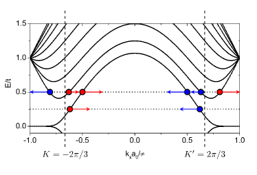
Figure 1: Electronic bandstructure of a zigzag GNR with $M=10$ horizontal chains along of width. $K$ and $K^{\prime}$ are the two inequivalent points of the first Brillouin zone of graphene. The left (right) arrows indicate positive (negative) group velocity and forward (backwards) electronic propagation.

The purpose of this work is to determine the fundamental mechanisms that lead to the PCC by directly analyzing the conductance dependence on the range of disorder as the scattering potential changes from short to long ranged. We have found that the PCC is not as robust as previous studies pointed out. In fact, we demonstrate that the emergence of the PCC crucially depends not only on the disorder range but also on the electronic energy.

This paper is organized as follows. In Sec. II we describe the tight-binding model with on-site energy disorder, the appearance of the PCC and the recursive Green’s functions method. The numerical results are shown in Sec. III, where we discuss the effect of the transition from short- to long-ranged disorder on the conductance $g$ (and also on the PCC). We also propose an analytical estimative for the degree of backscattering process to elucidate the physical origin of the PCC, which is compared to the conductance numerical results. Finally, Sec. IV is devoted to the conclusions.

II Model and theory

In this Section we present the model and the theory used to address the single-particle transport properties in GNRs. We first obtain analytical solutions for the band structure and wave functions of the tight-binding Hamiltonian that describes the electronic properties of pristine zigzag GNRs. Next, we introduce the local disorder model used to numerically study the conductance in GNRs. We close the Section with a brief description of the numerical method employed to calculate the transport properties, namely, the recursive Green’s functions method.

II.1 Tight-binding model

Close to half filling, the electrons in graphene are assumed to move by hopping through the $p_{z}$ orbitals of the carbon atoms. Using the labels introduced in Fig. 2, the first-neighbor tight-binding Hamiltonian for graphene reads

$$H=-t\sum_{n,m\in A}\bigg{(}a^{\dagger}_{n,m}b_{n,m+1}+a^{\dagger}_{n,m}b_{n-1,m}+$$

$$+\ a^{\dagger}_{n,m}b_{n+1,m}+\text{H.c.}\bigg{)},$$ (1)

where the hopping parameter is $t=2.7\ \text{eV}$ Castro Neto et al. (2009) and the sum is related to the sublattice $A$ sites only. The operators $a^{\dagger}_{n,m}\;(b^{\dagger}_{n^{\prime},m^{\prime}}$) create and $a_{n,m}\;(b_{n^{\prime},m^{\prime}}$) annihilate an electron at the site $(n,m)$ of the sublattice $A\,(B)$. The integers $n=1,2$ and $m=1,\ldots,M$ label the atomic sites in the GNR unit cell according to the notation established in Fig. 2. $M$ is related to the nanoribbon width by $W=Ma_{0}\sqrt{3}/2$. The lattice parameter $a_{0}=2.46\ \text{\r{A}}$ Castro Neto et al. (2009) relates to the carbon-carbon distance $a$ through $a_{0}=a\sqrt{3}$.

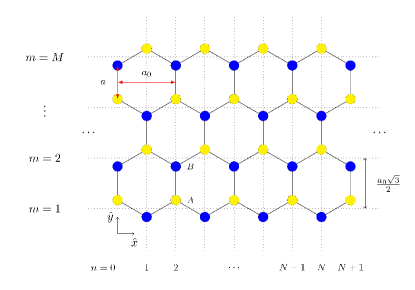
Figure 2: (Color online) Zigzag graphene ribbon geometry. $n$ and $m$ label the atomic sites on the sublattices $A$ (yellow dots) and $B$ (blue dots). The atoms labeled $n=1,\cdots,N$ belong to the ribbon region and the atoms $n=0$ and $n=N+1$ belong to the left and right contacts, respectively.

The zigzag edge boundary conditions are Brey and Fertig (2006)

$$a^{\dagger}_{n,0}|0\rangle =0,$$ (2)

$$b^{\dagger}_{n,M+1}|0\rangle =0,$$ (3)

where $|0\rangle$ is the vacuum state. Notice that we require the states of each sublattice to vanish at opposite edges.

The GNR eigenvalue problem reads

$$H\left|\alpha,k_{x}\right>=E_{\alpha}(k_{x})\left|\alpha,k_{x}\right>,$$ (4)

where $k_{x}$ is the longitudinal wavenumber and $\alpha$ the band (or channel) index. Using the on-site probability amplitudes $c_{\alpha;n,m}^{A}(k_{x})=\left<0\right|a_{n,m}\left|\alpha,k_{x}\right>$ and $c_{\alpha;n,m}^{B}(k_{x})=\left<0\right|b_{n,m}\left|\alpha,k_{x}\right>$ we write

$$\left|\alpha,k_{x}\right>=\sum_{n,m\in A}\left(c_{\alpha;n,m}^{A}(k_{x})a^{\dagger}_{\alpha;n,m}+c_{n-1,m}^{B}(k_{x})b^{\dagger}_{n-1,m}\right)\!\left|0\right>.$$ (5)

By inserting the eigenstates expansion (5) into the Eq. (1), one obtains K. Wakabayashi and Enoki (2010)

$$c_{\alpha;n,m}^{A}(k_{x}) ={\cal N}_{\alpha}(k_{x})e^{ina_{0}k_{x}/2}\sin\!\big{[}m\nu_{\alpha}(k_{x})\big{]},$$ (6)

$$c_{\alpha;n,m}^{B}(k_{x}) =\mp{\cal N}_{\alpha}(k_{x})e^{ina_{0}k_{x}/2}\sin\!\big{[}(m-M-1)\nu_{\alpha}(k_{x})\big{]},$$ (7)

where the minus and plus signs denote states with positive and negative energies, respectively. The normalization factor

$${\cal N}_{\alpha}(k_{x})=1/\sqrt{N\sum_{m=1}^{M}\sin^{2}\!\big{[}m\nu_{\alpha}(k_{x})\big{]}}$$ (8)

is obtained by imposing $\langle\alpha,k_{x}|\alpha,k_{x}\rangle=1$. The momentum function $\nu_{\alpha}(k_{x})$ is introduced to satisfy the boundary condition (3). $\nu_{\alpha}(k_{x})$ is given by the multiple solutions of the transcendental equation K. Wakabayashi and Enoki (2010); Brey and Fertig (2006)

$$2\cos(a_{0}k_{x}/2)=-\frac{\sin(M\nu_{\alpha})}{\sin\big{[}(M+1)\nu_{\alpha}\big{]}}.$$ (9)

These analytical solutions will be used in the calculation of the backscattering matrix elements. Finally, the zigzag GNR eigenergies read

$$E_{\alpha}(k_{x})/t=\pm\left|\frac{\sin[\nu_{\alpha}(k_{x})]}{\sin\!\big{[}(M+1)\nu_{\alpha}(k_{x})\big{]}}\right|.$$ (10)

II.2 Bulk disorder in GNR

We calculate the conductance of disordered GNRs of length $L=Na_{0}/2$ (Fig. 2). To treat disorder, with employ the Gaussian disorder model, defined as follows. We randomly choose $N_{\rm imp}$ sites as the centers of Gaussian potentials with range $d$. $N_{\rm imp}$ is expressed in terms of the impurity concentration $n_{\rm imp}=N_{\rm imp}/N_{\rm tot}$, where the total number of atoms in the scattering region is $N_{\rm tot}=NM$. Hence, the disorder potential $V$ at the position ${\bf r}$ reads

$$V({\bf r})=\sum_{i=1}^{N_{\rm imp}}U_{i}\,e^{-\left|{\bf r}-{\bf R}(n_{i},m_{i})\right|^{2}/d^{2}},$$ (11)

where ${\bf R}(n_{i},m_{i})$ is the center is the $i$th Gaussian disorder potential. The on-site lattice representation of $V$ is

$$V=\sum_{n,m\in A}\left(V_{n,m}a^{\dagger}_{n,m}a_{n,m}+V_{n-1,m}b^{\dagger}_{n-1,m}b_{n-1,m}\right),$$ (12)

where $V_{n,m}$ corresponds to $V({\bf r})$ evaluated at ${\bf R}(n,m)$ corresponding to the position of the lattice site $(n,m)$.

The potential amplitude $U_{i}$ is randomly chosen from a uniform distribution in the interval $|U_{i}|\leq U_{\rm max}$, where

$$U_{\rm max}=\frac{2}{\sqrt{3}}U_{0}/\left(\sum^{\text{full space}}_{\bf R}e^{-{\bf R}^{2}/d^{2}}\right).$$ (13)

The dimensionless parameter $U_{0}/t$ defines the maximum disorder potential energy at each impurity site.

II.3 Recursive Green’s function technique

The conductance is obtained by using the recursive Green’s functions method Fisher and Lee (1981); Kinnon (1985). This method provides a computationally efficient way to calculate the total Green’s function of a GNR connected to pristine semi-infinite graphene leads at both ends. Using a decimation method we compute the surface Green’s functions and the decay width functions of the left $\Gamma_{0}$ and right $\Gamma_{N+1}$ leads. Next, we split the GNR “central” region (of width $W$ and length $L$) in $N$ slices containing $M$ transversal sites [see Fig.2] and iteratively calculate the total retarded Green’s function $G^{r}_{1,N}$ that contains information about electron propagation from slice $1$ to $N$. Finally, the dimensionless conductance $g$ is obtained from the Caroli formula Caroli et al. (1971), namely, $g=\text{Tr}\left[\Gamma_{0}G^{r}_{1,N}\Gamma_{N+1}G^{a}_{1,N}\right]$. The linear electronic conductance is $G=(2e^{2}/h)g$, where the factor 2 is due to the spin degeneracy.

III Results

In this Section we study the robustness of the PCC in disordered zigzag GNRs. This is done by numerically computing the dimensionless conductance $g$ and interpreting the results in terms of the analytical tools presented in the previous Section.

We compute the dimensionless conductance averaged over a large number of disorder realizations $\langle g\rangle$ (typically $10^{3}$) by means of the recursive Green’s function method, The impurity potential strength is $U_{0}/t=1$. As in Ref. Wakabayashi et al., 2007, we consider GNRs with $M=10$. For a zigzag GNR of this width, there is a single propagating channel for $E<E_{2}\equiv 0.406t$, where we denote the threshold energy to open the $\alpha$th channel by $E_{\alpha}$.

Figure 3: Average dimensionless conductance $\langle g\rangle$ as a function of the potential range $d$ for a ribbon of length $L=500a_{0}$ and width $W=5\sqrt{3}a_{0}$ for the impurity concentrations (a) $n_{\rm imp}=0.10$ and (b) $n_{\rm imp}=0.01$.

We start by numerically investigating the behavior of the PCC in the crossover from SRD to LRD regimes as a function of the energy $E$. Figure 3 shows our results for $\langle g\rangle$ as a function of the potential range $d/a_{0}$ for two values of impurity concentration, namely, $n_{\rm imp}=0.10$ and $n_{\rm imp}=0.01$. The simulations show that for sufficiently large values of $d/a_{0}$, irrespective of $E$ and $n_{\rm imp}$, the PCC always occurs, as $\langle g\rangle=1$ within the numerical precision. Moreover, we find that the potential range $d_{c}$, defined as the potential range above which the PCC appears, depends strongly and non-monotonically on energy $E$: (i) $d_{c}$ decreases for increasing energies $E$ starting from the charge neutrality point, and (ii) $d_{c}$ increases with increasing energy as $E$ approaches $E_{2}$. This is in contrast to Ref. Wakabayashi et al., 2009, which suggests the emergence of the PCC for all energies $E<E_{2}$ at $d/a_{0}=1.5$ and $n_{\rm imp}=0.10$. The same qualitative trend is found for both low ($n_{\rm imp}=0.01$) and high ($n_{\rm imp}=0.10$) impurity concentrations we analyze, as shown in Figs. 3(b) and 3(a), respectively.

The overall values of the average conductance $\langle g\rangle$ are larger in the case of more diluted impurities, as expected. For both impurity concentrations, Fig. 3 shows conductance plateaus for short scattering potential ranges, typically $d/a_{0}\lesssim 0.3$. These plateaus have a simple interpretation. Let us consider a single Gaussian disorder scattering center, placed at a site $i$. For $d$ smaller than roughly half the inter-atomic distance $a/2=a_{0}/(2\sqrt{3})=0.29a_{0}$, the neighboring sites of $i$ are hardly affected by the scattering center placed at $i$. Further reduction in the potential range does not change the system Hamiltonian.

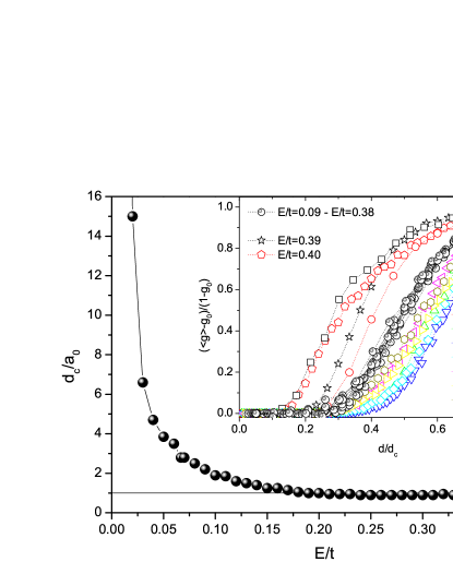
Figure 4: Disorder range above which the PCC appears, $d_{c}/a_{0}$, as a function of the electron energy $E$. Inset: Scaled average conductance $(\langle g\rangle-g_{0})/(1-g_{0})$ as a function of $d/d_{c}$ for different energies $E/t$.

To investigate the role of the disorder potential range on the emergence of the PCC, in Fig. 4 we show $d_{c}/a_{0}$, defined above, as a function of energy $E/t$ for $n_{\rm imp}=0.10$. Figure 4 shows that $d_{c}/a_{0}\approx 1$, except for low energies and energies at the threshold of the $n=2$ channel opening. The insert of Fig. 4 indicates that the behavior of the function $\langle g(d/a_{0})\rangle$ does not show, in general, a simple single-parameter scaling behavior. The numerical results suggests that a single-parameter scaling for $(\langle g\rangle-g_{0})/(1-g_{0})$ as a function of $d/d_{c}$ holds approximately true only for $0.15\lesssim E/t\lesssim 0.37$, where $g_{0}$ is the average conductance minimum for a fixed energy $E/t$.

To understand the numerical results presented above we investigate the backscattering mechanisms induced by the disorder potential. These mechanisms can be quantified by studying the backscattering matrix elements connecting forward- to backward-moving states with $\alpha=1$, namely,

$$\left\langle{1,-k_{x}}\right|V\left|{1,+k_{x}}\right\rangle=\sum_{n,m\in A}\bigg{\{}\left[c_{1;n,m}^{A}(-k_{x})\right]^{*}c_{1;n,m}^{A}(k_{x})V_{n,m}+\left[c_{1;n-1,m}^{B}(-k_{x})\right]^{*}c_{1;n-1,m}^{B}(k_{x})V_{n-1,m}\bigg{\}},$$ (14)

where the symbols are defined in Sec. II. The expression for the backscattering matrix element (14) becomes very simple in the SRD regime: For a case of a single impurity placed at ${\bf R}_{n_{0},m_{0}}$, it reads

$$\left\langle 1,-k_{x}(E)\right|V\left|1,+k_{x}(E)\right\rangle=\hskip 85.35826pt$$

$$=\left[c_{n_{0},m_{0}}^{\Lambda}(-k_{x})\right]^{*}c_{n_{0},m_{0}}^{\Lambda}(k_{x})V_{n_{0},m_{0}},$$ (15)

where $\Lambda=A$ or $B$.

Let us examine the backscattering matrix elements in a number of representative situations. We first consider the single-impurity scattering case. Figure 5 shows the backscattering matrix, Eq. (15), as a function of the energy for two different configurations: The Gaussian scattering potential is placed at the center or at the edge of the GNR. As for narrow zigzag GNRs and small values of $E$ the electronic states are typically concentrated at the edges of the ribbon, we expect a distinct behavior in these two limiting cases.

Figure 5(a) shows $V_{\rm back}(E)\equiv\left\langle 1,-k_{x}(E)\right|V\left|1,+k_{x}(E)\right\rangle$ as a function of $d/a_{0}$ for a single Gaussian potential placed at the center of the GNR. Due the SRD to LRD crossover, the backscattering matrix element decreases very fast as $d/a_{0}\gtrsim 1$. As expected from Eq. (15) and the previous discussion, $V_{\rm back}(E)$ hardly changes for $d/a_{0}\lesssim 0.25$. For $M=10$, the states $|1,\pm k_{x}\rangle$ become localized at the GNR edges when $E/t\lesssim 0.1$ Brey and Fertig (2006). In this situation, impurities located at the GNR center result in weak backscattering so that the plateaus quickly drop to $V_{\rm back}(E)\approx 0$. Figure 5(b) shows $|V_{\rm back}(E)|$ for the case of edge impurities. For $E/t>0.1$, corresponding to ordinary states, the behavior is similar to Fig. 5(a). However, for edge states the situation changes dramatically: Here $V_{\rm back}(E)$ decreases surprisingly slowly with increasing $d/a_{0}\gtrsim 1$. This indicates that, in the presence of edge states, intervalley scattering is highly sensitive to the impurity position, even in the LRD case.

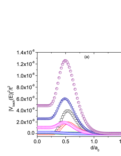
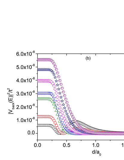
Figure 5: Backscattering matrix element $V_{\rm back}$ calculated as a function of the scattering range $d/a_{0}$ for different values of the energy $E$ for a single Gaussian impurity center placed (a) at the center of the GNR ($n_{0}=100,m_{0}=5$) and (b) at its edge vicinity ($n_{0}=100,m_{0}=9$). The GNR has the dimensions $N=200$ and $M=10$. For this value of GNR width, the edge state appears for $E<0.1t$. Wakabayashi et al. (2009); Brey and Fertig (2006)

We now consider the situations of low ($n_{imp}=0.01$) and large ($n_{imp}=0.10$) impurity concentrations, the same values used in the conductance numerical calculations (Fig. 3). We compute the backscattering matrix element using Eq. (14) and their average over different configurations of disorder. The results are shown in Fig. 6 and are contrasted with the average conductance $\langle g\rangle$. Like $\langle g\rangle$, the average backscattering matrix elements, $\langle|V_{\rm back}(E)|^{2}\rangle$, also display a plateau-like behavior for $d/a_{0}<0.3$. For $|E|>0.15t$, $\langle|V_{\rm back}(E)|^{2}\rangle$ exhibits a fast decay with increasing $d/a_{0}$ independent of the energy $E$. On the other hand, for $|E|<0.15t$ the backscattering matrix elements decay nearly exponentially for $1.0\lesssim d/a_{0}\lesssim 2.0$, reaching minimum values depending on $n_{\rm imp}$. For energies near the Dirac point ($E=0$), backscattering is maximal, persisting even in the LRD regime. In summary, in the SRD regime the averaged backscattering reaches its maximum value causing a conductance suppression. In distinction, in general $\langle|V_{\rm back}(E)|^{2}\rangle$ is suppressed in the LRD favoring the appearance of the PCC provided $d/a_{0}\gtrsim 1$.

The small energy regime is an exception to this picture: The enhanced backscattering near the charge neutrality point can be understood in simple terms. Qualitatively, one expects that a scattering potential with a characteristic length scale $d$ can only effectively backscatter electron states with initial momentum $k$ to final momentum $-k$ provided $1/d\approx|\!-2k+G|$, where $G$ is a reciprocal lattice vector. Nonzero $G$ vectors describe Umklapp scattering processes. As one approaches the charge neutrality point, scattering between $k\approx\pi/a$ to $-k\approx-\pi/a$ mediated by a $G=2\pi/a$ Umklapp becomes dominant, so that $|\!-2k+G|$ approaches zero and even a very smooth potential (large $d$) is able to scatter the electron states and destroys PCC. That is the reason for the sharp increase of $d_{c}$ near $E=0$, shown in Fig. 4.

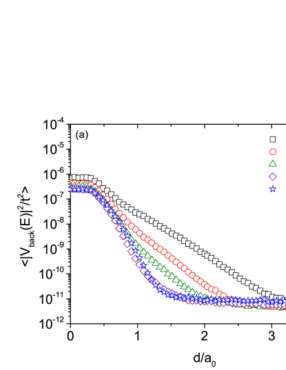
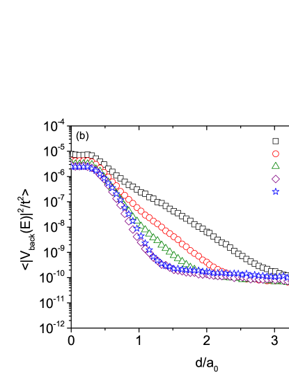
Figure 6: Average backscattering matrix element $\langle|V_{\rm back}|^{2}\rangle$ as a function of the disorder range $d/a_{0}$ for a number of energies $E$. The average is taken over $10^{3}$ disorder configurations for an impurity concentration of (a) $n_{imp}=0.01$ and (b) $n_{imp}=0.10$. The GNR has the dimensions $L=500a_{0}$ and $W=10(\sqrt{3}/2)a_{0}$. This ribbon presents edge state for $E<0.1t$.

We discuss now the robustness of the PCC for energies $E$ approaching $E_{2}$. As discussed, for such energies $V_{\rm back}\approx 0$ as long as $d/a_{0}\gtrsim 1$. To explain deviations from the PCC, first-order perturbation theory is not sufficient since LRD cannot account for the large momentum transfer necessary for backscattering, as already discussed. LRD can only account for backscattering processes in the vicinities of the energy $E_{2}$, where left and right propagating modes (Fig. 1) are not far away in momentum space. For a sufficiently smooth long-range disorder, one can account for disorder effects by introducing a local chemical potential as $\mu[V({\bf r})]$. In this scenario, LRD can suppress the PCC at energies $E_{2}-\delta E\lesssim E\lesssim E_{2}+\delta E$, where $\delta E$ is the typical disorder potential fluctuation.

We have also carried out numerical simulations for higher energies (up to $E/t=0.9$), corresponding to the multi-channel case. However, in this case we have not found any qualitative difference between our results and the ones reported in Ref. Wakabayashi et al., 2009. More precisely, we have found deviations from the PCC for incident energies at the vicinity of energies corresponding to the crossover between $g=2n-1$ and $2n+1$ for clean ribbons ($n$ being the number of channels). This behavior corroborates the results of Ref. Wakabayashi et al., 2009.

IV Conclusions

In summary, the electronic conductance of disordered GNRs in general, and the emergence of the PCC in particular, present a richer behavior than expected from previous studies. Specifically, the critical impurity potential $d_{c}$ for the PCC emergence shows a strong and clear dependence on the electronic energy. This result, obtained numerically from recursive Green’s functions calculations, is explained in simple physical grounds by calculations of energy and potential range dependences of electron intervalley scattering probabilities, which follows the opposite qualitative trends of the conductance. This occurs for sufficiently low energies such that the Fermi level crosses just one band (single channel conductance). This behavior confirms and justifies the simple picture of an electron undergoing intervalley scattering only if the impurity potential has substantial Fourier components at large momenta, thus being able to provide a momentum transfer $\Delta k\approx 1/a_{0}$ to the electron. In other words, for a single channel, backscattering occurs only if intervalley scattering does. This picture not only explains the conductance behavior for low energies, but it also provides us with guidelines to explain the more complicated cases in which the Fermi level crosses many channels. In that case, as shown in Fig. 1, backscattering (i.e., group velocity reversal) can occur even for small momentum transfers (intravalley scattering), therefore explaining the disappearance of the PCC as the Fermi level approaches the threshold for opening the second transmission channel.