Long-range interactions in the ozone molecule: spectroscopic and dynamical points of view

Abstract

Using the multipolar expansion of the electrostatic energy, we have characterized the asymptotic interactions between an oxygen atom O$(^{3}P)$ and an oxygen molecule O${}_{2}(^{3}\Sigma_{g}^{-})$, both in their electronic ground state. We have calculated the interaction energy induced by the permanent electric quadrupoles of O and O₂ and the van der Waals energy. On one hand we determined the 27 electronic potential energy surfaces including spin-orbit connected to the O$(^{3}P)$ + O${}_{2}(^{3}\Sigma_{g}^{-})$ dissociation limit of the O–O₂ complex. On the other hand we computed the potential energy curves characterizing the interaction between O$(^{3}P)$ and a O${}_{2}(^{3}\Sigma_{g}^{-})$ molecule in its lowest vibrational level and in a low rotational level. Such curves are found adiabatic to a good approximation, namely they are only weakly coupled to each other. These results represent a first step for modeling the spectroscopy of ozone bound levels close to the dissociation limit, as well as the low energy collisions between O and O₂ thus complementing the knowledge relevant for the ozone formation mechanism.

I Introduction

The ozone molecule plays a crucial role in the physics and chemistry of the Earth atmosphere. However, a lot remains to be understood, especially about its formation, which is thought to take place in two steps schinke2006 . Firstly, an oxygen atom O and an oxygen molecule O₂ collide to give a ro-vibrationally or electronically excited ozone complex O${}_{3}^{*}$. Secondly, this complex stabilizes by inelastic collision with one surrounding atom or molecule, which is the so-called deactivation process. However, this second step takes place provided that the excited complex O${}_{3}^{*}$ does not dissociate into O$+$O₂ before colliding with the surrounding gas. Characterizing the competition between deactivation on the one hand, and dissociation on the other hand, is the key point in order to understand quantitatively the ozone formation in the atmosphere.

In this respect, one of the most striking features of ozone physical chemistry is the unconventional isotopic effects that influence the competition between stabilization and dissociation of O${}_{3}^{*}$ thiemens1983 ; mauersberger1987 ; anderson1997 ; janssen2001 ; mauersberger2005 . It became clear in recent years janssen1999 , that these isotopic effects were determined by the difference of zero-point energies $\Delta\textrm{ZPE}$ of the O₂ isotopologues in the entrance and the dissociation channels. If $\Delta\textrm{ZPE}>0$, dissociation is energetically unfavorable: the O${}_{3}^{*}$ has a higher lifetime, and so is more likely to give stable O₃. On the contrary, if $\Delta\textrm{ZPE}<0$, dissociation is energetically favorable, and it tends to dominate stabilization.

The unconventional isotopic effects were very well understood in the beginning of the 2000’s within the framework of the statistical RKRM (Rice-Kassel-Ramsperger-Marcus) theory gao2001 ; gao2002 . However, an adjustable parameter $\eta$ had to be added to that theory, in order to account for deviation from the energy equipartition theorem, after the formation of the O${}_{3}^{*}$ molecule. Then, the need for first-principle studies of the ozone formation, especially based on quantum mechanics, became obvious. Since a full quantum treatment of the two-step process is beyond the possibilities offered by current computers, researchers are urged to focus on precise aspects of the process, e.g. highly-excited vibrational levels of O₃ grebenshchikov2003 ; babikov2003 ; lee2004 , the influence of resonances babikov2003b ; grebenshchikov2009 , or to use less demanding computational techniques, e.g. classical-trajectory fleurat2003 or mixed-quantum-classical calculations ivanov2012 .

The common features of all those studies is that they need a reliable potential energy surface (PES), at least for the electronic ground state $\tilde{X}^{1}A_{1}$. Since the formation of stable O₃ involves a wide variety of geometries, from almost separated O and O₂, to tightly bound O₃, one actually needs a global PES. Up to now, all the published PESs share the same general features. In particular when they are cut along the minimum-energy path, they all show a change in character between the inner and the asymptotic regions, which is due to an avoided crossing with an excited electronic state, also referred to as the transition state. However, there is still a controversy on whether this avoided crossing induces a potential barrier that goes above siebert2001 ; siebert2002 or below the dissociation limit rosmus2002 ; babikov2003b ; holka2010 , or on the contrary, a monotonic evolution of the potential energy as suggested by the most recent ab initio calculations dawes2011 .

Up to now, all the articles that aimed at describing the O$-$O₂ asymptotic region were based on quantum-chemical calculations of the ground-state and possibly the lowest excited-states PESs of O₃ rosmus2002 ; tashiro2003 . In the present paper, we propose an alternative method based on the multipolar expansion of the electrostatic potential energy between O and O₂, both in their electronic ground state. This method enables us to obtain, in a single calculation, the 27 spin-orbit PESs connected to the dissociation threshold O$(^{3}P)+$O${}_{2}(X^{3}\Sigma_{g}^{-})$. The calculated PESs are then functions of the electric properties, i.e. multipole moments and multipole polarizabilities, of the separated systems. This method is valid provided that the electronic clouds of O and O₂ do not overlap, that is for a O–O₂ distance larger than 8 Bohr. Such asymptotic PESs can then be used as a tool to check the quality of the ab initio PESs.

In this article, we use two complementary approaches to characterize the O$-$O₂ long-range interactions. In section II, we consider the atom and the diatom at fixed geometries, that is at given inter-particle distances and bending angles. The obtained PESs can be directly connected to ab initio PESs. In section III, we include in our model the vibration and rotation of O₂ which yields one-dimensional potential energy curves (PECs) depending on the O–O₂ distance. Such curves are relevant for the low energy dynamics of the O–O₂ complex, in particular to which extent the rotation of O₂ is hindered by the presence of O. These curves are also useful for modeling the vibrational levels of ozone close to its dissociation limit grebenshchikov2003 ; babikov2003 ; lee2004 . We discuss in section IV the way to connect both approaches which is done for the first time, to the best of our knowledge. Section V contains our conclusions and prospects.

II Asymptotic electronic potential energy surfaces between O and O₂

As the two ground state particles O and O₂ are far away from each other, i.e. their electronic clouds do not overlap, we use the Jacobi coordinates to describe the PESs. The body-fixed frame associated to the O–O₂ complex has its $z$ axis connecting O to the center of mass of O₂. The $x$ axis is perpendicular to the $z$ axis and is located in the plane of the three atoms; the $y$ axis is perpendicular to this plane. We also introduce the coordinate system $x_{d}y_{d}z_{d}$ linked to the O₂ diatom. The axes $z_{d}$ and $x_{d}$ are related to $z$ and $x$ by a rotation of angle $\theta$ about the $y_{d}\equiv y$ axis. We denote as $r$ the interatomic distance in the O₂ molecule, and $R$ the distance between the O atom and the center of mass of O₂. The formalism presented in this section allows for calculating three-dimensional PESs depending on $R$, $r$ and $\theta$. In the following, we set $r\equiv r_{e}=2.282a_{0}$ ($a_{0}=0.0529177$ nm is the Bohr radius and the atomic unit for distances) at the equilibrium distance of O₂ without loss of generality for our purpose.

II.1 Model

The calculations below are based on the formalism described in Ref. bussery-honvault2008 , and used in Ref. bussery-honvault2009 . The quantities referring to O and O₂ are respectively characterized by the subscripts “$a$” after “atom” and “$d$” after “diatom”. The starting point of our model is the multipole expansion in inverse powers of $R$ of the electrostatic energy between two charge distributions “$a$” and “$d$” (see bussery-honvault2008 , Eqs. (2) and (3))

$$\hat{V}_{ad}=\sum_{\ell_{a}\ell_{d}}\frac{1}{R^{1+\ell_{a}+\ell_{d}}}\sum_{m=-\ell_{<}}^{+\ell_{<}}g_{m}(\ell_{a},\ell_{d})\hat{Q}_{\ell_{a}}^{m}\hat{Q}_{\ell_{d}}^{-m}$$ (1)

with $\ell_{<}=\min(\ell_{a},\ell_{d})$ and lepers2010

$$g_{m}(\ell_{a},\ell_{d})=\frac{(-1)^{\ell_{d}}(\ell_{a}+\ell_{d})!}{\sqrt{(\ell_{a}+m)!(\ell_{a}-m)!(\ell_{d}+m)!(\ell_{d}-m)!}}.$$ (2)

In Eq. (1), $\hat{Q}_{\ell_{a}}^{m}$ ($\hat{Q}_{\ell_{d}}^{-m}$) is the $\ell_{a}$- ($\ell_{d}$-) rank and $m$-($-m$-)component multipole-moment operator of the atom (diatom) expressed in the $xyz$ coordinate system. The multipole moments of the diatom is conveniently expressed as

$$\hat{Q}_{\ell_{d}}^{-m}=\sum_{m_{d}=-\ell_{d}}^{+\ell_{d}}d_{-mm_{d}}^{\,\ell_{d}}(\theta)\hat{q}_{\ell_{d}}^{m_{d}}\,,$$ (3)

where $\hat{q}_{\ell_{d}}^{m_{d}}$ is the multipole moment operator of the diatom expressed in the $x_{d}y_{d}z_{d}$ coordinate system, and $d_{-mm_{d}}^{\,\ell_{d}}(\theta)$ is the reduced Wigner function, which characterizes the rotation from the $x_{d}y_{d}z_{d}$ to the $xyz$ frame.

The multipolar expansion (1) is valid provided that the electronic wave functions of O and O₂ do not overlap. This condition is fulfilled for distances $R$ larger than the so-called LeRoy radius leroy1974 $R_{LR}=2\{\sqrt{\langle r^{2}\rangle_{\mathrm{O}}}+\sqrt{\langle r^{2}\rangle_{\mathrm{O}_{2}}}\}\approx 8a_{0}$, where the mean squared radius of the electronic wave function in O is $\langle r^{2}\rangle_{\mathrm{O}}=2.001a_{0}$. The quantity $\sqrt{\langle r^{2}\rangle_{\mathrm{O}_{2}}}\approx r_{e}/2+\langle r\rangle_{\mathrm{O}}$ is roughly evaluated from the equilibrium distance $r_{e}=2.282a_{0}$ of O₂ and the mean radius of the electronic wave function in O $\langle r\rangle_{\mathrm{O}}=1.24a_{0}$.

In this work, we calculate the two leading terms of the $R^{-n}$ expansion for $R>R_{LR}$: the first-order term reflecting the interaction between the permanent quadrupole moments of O and O₂ ($\ell_{a}=\ell_{d}=2$) scaling as $R^{-5}$, and the second-order (Van der Waals) term related to the interaction between the induced dipole moments ($\ell_{a}=\ell_{d}=1$) scaling as $R^{-6}$. While generally tedious to obtain from ab initio calculations higher-order contributions may also be significant around $R_{LR}$. For instance, assuming that the maximal values of the $C_{6}$ and $C_{8}$ coefficients for the O-O₂ interaction are half of those for $O_{2}$-$O_{2}$ bartolomei2010 ) we obtain $C_{6}\approx 31$ a.u. (close to the values obtained in the present work, see next section) and $C_{8}\approx 1291$ a.u.. At $R=8a_{0}$ the $C_{8}$ term would then represent at most 64% of the $C_{6}$ one and 41% at $R=10a_{0}$. Therefore our work provides the essentials of the long-range interaction between O and O₂. In order to match the present asymptotic expansions to the ab initio calculations, the safest way is to use the $C_{5}$ and $C_{6}$ values determined below to fit the long-range part of the ab initio PESs beyond $R_{LR}$ and to extract the related higher-order terms. Another possibility would be to directly compute the next term $C_{8}$, but this beyond the scope of the present paper.

II.1.1 Zeroth-order energies and state vectors

The oxygen atom is in an arbitrary fine-structure level $\left|J_{a}M_{a}\right\rangle$ of its ground state ${}^{3}P_{J_{a}M_{a}}$, where $J_{a}$ is the total angular momentum with projection $M_{a}$ on the $z$ axis, resulting from the sum of the projections $M_{L_{a}}$ and $M_{S_{a}}$ of the orbital $L_{a}$ and spin $S_{a}$ angular momenta of the atom, respectively. Since the spin-orbit constant $A_{O}$ of oxygen is negative ($A_{O}=-79.1$  cm^-1), the ${}^{3}P_{2}$ fine-structure level is the lowest in energy.

The ground electronic state ${}^{3}\Sigma_{g}^{-}$ of O₂ has an orbital angular momentum projection $\Lambda_{d}=0$ on the $z_{d}$ axis and a spin $S_{d}=1$ with projection $\Sigma_{d}$ on $z_{d}$. The fine structure in the O₂ energy spectrum induced by the spin-spin interaction writes

$$\left\langle\Lambda_{d}S_{d}\Sigma_{d}\left|\hat{H}_{SS}\right|\Lambda_{d}S_{d}\Sigma_{d}\right\rangle = \left\langle\frac{\lambda}{2}\left(3\hat{S}_{z_{d}}^{2}-\hat{\mathbf{S}}^{2}\right)\right\rangle$$ (4)

$$= \frac{\lambda(r)}{2}\left(3\Sigma_{d}^{2}-S_{d}\left(S_{d}+1\right)\right),$$

where $\lambda(r)$ is the ($r$-dependent) spin-spin constant, with $\lambda(r_{e})=1.980$ cm^-1 tinkham1955 . The interaction between the electric multipole moments of O and O₂ only depends on the spatial coordinates of the electrons and the nuclei so that we will ignore the O₂ fine structure in the following. Assuming an energy origin at the ${}^{3}P_{2}$ oxygen level and at the O₂ ground level, the zeroth-order energy is

$$E_{0}=\frac{A_{O}}{2}\left(J_{a}\left(J_{a}+1\right)-6\right),$$ (5)

corresponding to the unperturbed state vectors $|\Psi_{0}\rangle=\left|J_{a}M_{a}\right\rangle\left|\Lambda_{d}\Sigma_{d}\right\rangle$.

II.1.2 First-order quadrupole-quadrupole interaction

The first-order quadrupole-quadrupole interaction is obtained by setting $\ell_{a}=\ell_{d}=2$ and $n=5$ in Eq. (3) of Ref. bussery-honvault2008 . Since $L_{a}=S_{a}=1$, we can rewrite Eqs. (4)-(5) of Ref. bussery-honvault2008 as

$$E_{\mathrm{elec}}^{\,J_{a}M_{a}J^{\prime}_{a}M^{\prime}_{a}\Lambda_{d}\Sigma_{d}\Lambda^{\prime}_{d}\Sigma^{\prime}_{d}}(r,R,\theta)$$ (6)

$$= \frac{1}{R^{5}}\delta_{\Sigma_{d}\Sigma^{\prime}_{d}}\sum_{M_{L_{a}}M_{S_{a}}}C_{1M_{L_{a}}1M_{S_{a}}}^{J_{a}M_{a}}$$

$$\times \sum_{M^{\prime}_{L_{a}}M^{\prime}_{S_{a}}}C_{1M^{\prime}_{L_{a}}1M^{\prime}_{S_{a}}}^{J^{\prime}_{a}M^{\prime}_{a}}\delta_{M_{S_{a}}M^{\prime}_{S_{a}}}$$

$$\times {}^{ii^{\prime}jj^{\prime}}V_{52mm_{d}}^{\,\mathrm{elec}}(r)d_{-mm_{d}}^{2}(\theta),$$

where $m_{d}$ refers to the components of the 2-rank tensor in the diatom frame, $C_{a\alpha b\beta}^{c\gamma}=\langle a\alpha b\beta|c\gamma\rangle$ is the compact expression of Ref. varshalovich1988 for the Clebsch-Gordan coefficients, and where

$${}^{ii^{\prime}jj^{\prime}}V_{52mm_{d}}^{\,\mathrm{elec}}(r)=g_{m}(\ell_{a},\ell_{d})\langle 1M_{L_{a}}|\hat{Q}_{2}^{m}|1M^{\prime}_{L_{a}}\rangle\langle\Lambda_{d}|\hat{q}_{2}^{m_{d}}(r)|\Lambda^{\prime}_{d}\rangle\,.$$ (7)

The superscripts $i,i^{\prime}$ and $j,j^{\prime}$ designate in a compact way the quantum numbers of O and O₂, respectively, i.e. $i=\{L_{a}=1,M_{L_{a}}\}$, $i^{\prime}=\{L^{\prime}_{a}=1,M^{\prime}_{L_{a}}\}$, $j=\{\Lambda_{d}=0,\Sigma_{d}\}$ and $j^{\prime}=\{\Lambda^{\prime}_{d}=0,\Sigma^{\prime}_{d}\equiv\Sigma_{d}\}$. As the O₂ electronic ground state is of $\Sigma$ symmetry the only non-zero component of the quadrupole operator is $q(r)=\left\langle\Lambda_{d}=0\right|\hat{q}_{2}^{m_{d}=0}\left|\Lambda_{d}=0\right\rangle$. In Eq. (7) we only keep the quantum numbers which are not fixed: ${}^{ii^{\prime}jj^{\prime}}V_{52mm_{d}}^{\,\mathrm{elec}}$ and $E_{\mathrm{elec}}^{\,J_{a}M_{a}J^{\prime}_{a}M^{\prime}_{a}\Lambda_{d}\Sigma_{d}\Lambda^{\prime}_{d}\Sigma^{\prime}_{d}}$ can be simplified to ${}^{M_{L_{a}}M^{\prime}_{L_{a}}}V_{52mm_{d}}^{\,\mathrm{elec}}$ and $E_{\mathrm{elec}}^{\,J_{a}M_{a}J^{\prime}_{a}M^{\prime}_{a}}$ respectively.

Using the Wigner-Eckart theorem, we can connect all matrix elements of O quadrupole moment to a single one, say that for which $M_{L_{a}}=M^{\prime}_{L_{a}}=m=0$,

$$\left\langle 1M_{L_{a}}\right|\hat{Q}_{2}^{m}\left|1M^{\prime}_{L_{a}}\right\rangle=\left(-1\right)^{M_{L_{a}}}\sqrt{\frac{15}{2}}\left(\begin{array}[]{ccc}1&2&1\\ -M_{L_{a}}&m&M^{\prime}_{L_{a}}\end{array}\right)Q\,,$$ (8)

with $Q=\langle 10|\hat{Q}_{2}^{0}|10\rangle$, and where the symbol $(...)$ is a Wigner 3-j symbol, which imposes $M_{L_{a}}=M^{\prime}_{L_{a}}+m$.

II.1.3 Second-order dipole-dipole interaction

The second-order interaction scales as $R^{-6}$ and results from the dispersion term due to the induced dipole-induced dipole interaction. It is calculated by setting $\ell_{a}=\ell^{\prime}_{a}=\ell_{d}=\ell^{\prime}_{d}=1$ and $n=6$ in Eqs. (6)-(10) of Ref. bussery-honvault2008 . In this case, the coupled polarizabilities (Eq. (7) of Ref. bussery-honvault2008 ) are tensors which can be of rank $\mathcal{L}_{a}=0$, 2 and $\mathcal{L}_{d}=0$, 2, for O and O₂ respectively. Then, the dispersion energy (see Eq. (8) of Ref. bussery-honvault2008 ) can be written as a sum of an isotropic ($\mathcal{L}_{d}=0$, i.e. $\theta$-independent) and an anisotropic contribution ($\mathcal{L}_{d}=2$, i.e. $\theta$-dependent)

$$E_{\mathrm{disp}}^{\,J_{a}M_{a}J^{\prime}_{a}M^{\prime}_{a}}(r,R,\theta) = -\frac{1}{R^{6}}\delta_{\Sigma_{d}\Sigma^{\prime}_{d}}\sum_{M_{L_{a}}M_{S_{a}}}C_{1M_{L_{a}}1M_{S_{a}}}^{J_{a}M_{a}}$$ (9)

$$\times \sum_{M^{\prime}_{L_{a}}M^{\prime}_{S_{a}}}C_{1M^{\prime}_{L_{a}}1M^{\prime}_{S_{a}}}^{J^{\prime}_{a}M^{\prime}_{a}}\delta_{M_{S_{a}}M^{\prime}_{S_{a}}}$$

$$\times \left({}^{M_{L_{a}}M^{\prime}_{L_{a}}}V_{6000}^{\mathrm{disp}}(r)+\sum_{\mathcal{M}=-\mathcal{L}_{<}}^{\mathcal{L}_{<}}\sum_{\mathcal{M}_{d}=-2}^{2}{}^{M_{L_{a}}M^{\prime}_{L_{a}}}V_{62\mathcal{MM}_{d}}^{\mathrm{disp}}(r)d_{-\mathcal{MM}_{d}}^{2}(\theta)\right),$$

with $\mathcal{L}_{<}=\min(\mathcal{L}_{a},\mathcal{L}_{d}=2)\equiv\mathcal{L}_{a}$. Note that in Eq. (9), the labels for $E_{\mathrm{disp}}$ and $V^{\mathrm{disp}}$ have been simplified in the same way as for the first-order term (see text after Eq. (7)).

The dispersion coefficients ${}^{M_{L_{a}}M^{\prime}_{L_{a}}}V_{6\mathcal{L}_{d}\mathcal{MM}_{d}}^{\mathrm{disp}}$ (given by Eq. (9) of Ref. bussery-honvault2008 ) depend on dynamical polarizabilities at imaginary frequencies. They are conveniently expressed in terms of coupled polarizabilities for O and O₂ respectively, following the definitions introduced in Ref. spelsberg1993

$${}^{M_{L_{a}}M^{\prime}_{L_{a}}}\alpha_{(11)\mathcal{L}_{a}\mathcal{M}}(i\omega)=\sum_{mm^{\prime}}\langle 1m1m^{\prime}|\mathcal{L}_{a}\mathcal{M}\rangle{}^{M_{L_{a}}M^{\prime}_{L_{a}}}\alpha_{1m1m^{\prime}}(i\omega),$$ (10)

$$\alpha_{(11)\mathcal{L}_{d}\mathcal{M}_{d}}(i\omega;r)=\sum_{qq^{\prime}}\langle 1q1q^{\prime}|\mathcal{L}_{d}\mathcal{M}_{d}\rangle\alpha_{1q1q^{\prime}}(i\omega;r)$$ (11)

The uncoupled dynamic polarizabilities ${}^{M_{L_{a}}}\alpha_{1010}\equiv^{M_{L_{a}}}\alpha_{zz}$ for the $M_{L_{a}}$ sublevels of O$(^{3}P)$ assuming an electric field polarized in the $z$ direction

$${}^{M_{L_{a}}}\alpha_{zz}(i\omega)=\frac{\sum_{k=0}^{N-1}({}^{M_{L_{a}}}a_{k})\times(i\omega)^{2k}}{1+\sum_{k=1}^{N}({}^{M_{L_{a}}}b_{k})\times(i\omega)^{2k}},$$ (12)

have been calculated by one of us using [N,N-1] Padé approximants $({}^{M_{L_{a}}}a_{k})$ and $({}^{M_{L_{a}}}b_{k})$ langhoff1970 reported in the supplementary material epaps for convenience, and published elsewhere stoecklin2012 . For O(${}^{3}P$) we obtain

$${}^{M_{L_{a}}M^{\prime}_{L_{a}}}\alpha_{(11)00}(i\omega) = -\frac{{}^{M_{L_{a}}=0}\alpha_{zz}(i\omega)+2{}^{M_{L_{a}}=\pm 1}\alpha_{zz}(i\omega)}{\sqrt{3}}$$ (13)

$${}^{M_{L_{a}}M^{\prime}_{L_{a}}}\alpha_{(11)2\mathcal{M}}(i\omega) = \left(-1\right)^{1-M_{L_{a}}}\sqrt{5}\left(\begin{array}[]{ccc}1&2&1\\ -M_{L_{a}}&\mathcal{M}&M^{\prime}_{L_{a}}\end{array}\right)$$ (17)

$$\times\left({}^{M_{L_{a}}=\pm 1}\alpha_{zz}(i\omega)-{}^{M_{L_{a}}=0}\alpha_{zz}(i\omega)\right)\,.$$

Similarly the coupled dynamical polarizabilities of O₂ $\alpha_{(11)\mathcal{L}_{d}\mathcal{M}_{d}}$ are related to the ($r$-dependent) uncoupled ones $\alpha_{1010}(i\omega;r)=\alpha^{\parallel}(i\omega;r)$ (the parallel component along $z_{d}$) and $\alpha_{111-1}(i\omega;r)=-\alpha^{\bot}(i\omega;r)$ (the perpendicular component with respect to $z_{d}$) according to bussery-honvault2008

$$\alpha_{(11)00}(i\omega;r) = -\frac{\alpha^{\parallel}(i\omega;r)+2\alpha^{\bot}(i\omega;r)}{\sqrt{3}}$$ (18)

$$\alpha_{(11)2\mathcal{M}_{d}}(i\omega;r) = \sqrt{\frac{2}{3}}\delta_{\mathcal{M}_{d}0}\left(\alpha^{\parallel}(i\omega;r)-\alpha^{\bot}(i\omega;r)\right).$$ (19)

Note that just like $m_{d}$ (see Eqs. (6) and (7)), $\mathcal{M}_{d}$ is zero because O₂ is in a $\Sigma$ electronic state.

II.2 Asymptotic PESs: results and discussions

Table 1: Quadrupole moment $Q$ and static dipole polarizabilities ${}^{M_{L_{a}}}\alpha_{zz}(\omega=0)$ (in a.u.) for O(³P). All values are expressed in atomic units.

Ref.	$Q$	${}^{M_{L_{a}}=0}\alpha_{zz}$	${}^{M_{L_{a}}=1}\alpha_{zz}$
This worka	-0.95	5.64	4.83
Ref.Gutsev1998 b	-0.95	-	-
Ref.Das1998 c	-	5.86	4.94
Ref.Medved2000 d	-1.02	5.91	4.89
Ref.Medved2000 e	-1.04	6.08	4.99

^aFull valence CASSCF(6e,5o) with aug-cc-pVQZ basis set
^bCCSD(T) with aug-cc-pV5Z basis set
^cCCSD(T) with quadruple-$\zeta$ GTO/CGTO basis set 
^dCASSCF and ^eCASPT2 both with triple-$\zeta$ GTO/CGTO basis set

Table 2: Quadrupole moment $q$, and parallel $\alpha^{\parallel}(\omega=0)$ and perpendicular $\alpha^{\bot}(\omega=0)$ static dipole polarizabilities (in a.u.) for O₂(X${}^{3}\Sigma^{-}_{g}$). All values calculated ab initio are given at the equilibrium distance $r_{e}=2.282$ a.u. and are expressed in atomic units. The value in parenthesis is calculated for for the lowest vibrational level following Ref. lawson1997 .

Method	$q$	$\alpha^{\parallel}$	$\alpha^{\perp}$
Ref. lawson1997 a	-0.2530 (-0.2273)
Ref. kumar1996 b		15.29	8.24
Ref. bartolomei2010 c	-0.2251	15.367	8.228
Experimental	-0.3$\pm$0.1d	15.7$\pm$0.3e	8.4$\pm$0.3e
	-0.25f	15.37g	8.22g

^a CBS-CASSCF+1+2
^bsemi-empirical DOSD values
^cRecommended values: CAS(12e-14o)-ACPF calc. with aug-cc-pV5Z basis set
^doptical birefringence Buckingham1968
^evibration rotation Raman spectroscopy Buldakov1996
^fpressure-induced far-infrared spectrum Cohen1977
^gdepolarization ratios Bridge1966

We have calculated the permanent quadrupole moment $Q$ of O(${}^{3}P$) (see Eq. (8)), with the CASSCF method, in a full-valence active space including 6 electrons and 5 orbitals and an ”aug-cc-pVQZ” basis set. Our value $Q=-0.95$ a.u., is in very good agreement with the value obtained with the CCSD(T) using quadruple-$\zeta$ (or higher) basis set Gutsev1998 of similar quality to the one presently used (Table 1). This indicates that the contribution of dynamical electron correlation effects which are missing in our CASSCF treatment can safely be neglected, provided that sufficiently large basis sets and active space are used. Only static dipole polarizabilities ($\omega=0$) have been reported up to now in the literature, and Table 1 shows that our value obtained from Eq. (12) is in satisfactory agreement with other published values.

The available values of the permanent quadrupole moment and static dipole polarizabilities of O₂(X${}^{3}\Sigma^{-}_{g}$) are shown in Table 2. In the present work, the quadrupole moment $q(r)=\left\langle\Lambda_{d}=0\right|\hat{q}_{2}^{0}\left|\Lambda_{d}=0\right\rangle$ is taken from Ref. lawson1997 , where it is calculated at the equilibrium distance $r_{e}=2.282$ a.u. and for the lowest vibrational level $v_{d}=0$ using an harmonic-oscillator approximation. The dynamic dipole polarizabilities are taken from the semi-empirical dipole-oscillator-strength distribution (DOSD) values of Ref. kumar1996 . All quantities regarding O₂ are in good agreement with the best recommended ab initio values of Ref. bartolomei2010 as well as with experimental values.

Table 3: Long-range non-zero ${}^{M_{L_{a}}M^{\prime}_{L_{a}}}V^{\mathrm{elec}}_{52m0}$ electrostatic coefficients (in atomic units, see Eq. (7)) for the O(${}^{3}P$) + O₂(X${}^{3}\Sigma^{-}_{g}$) interaction at $r=r_{e}=2.282$ a.u. and for the lowest vibrational level $v_{d}=0$ using the data of Table 2.

$M_{L_{a}}$	$M^{\prime}_{L_{a}}$	$m$	$V_{5}^{\rm elec}(r_{e})$	$V_{5}^{\rm elec}(v_{d}=0)$
$\pm$1	$\pm$1	0	-0.721	-0.647
$\pm$1	0	$\pm$1	0.832	0.748
$\pm$1	$\mp$1	$\pm$2	-0.294	-0.264
0	$\pm$1	$\mp$1	-0.832	-0.748
0	0	0	1.442	1.295

Table 4: Long-range non zero ${}^{M_{L_{a}}M^{\prime}_{L_{a}}}V^{\mathrm{disp}}_{6\mathcal{L}_{d}\mathcal{M}0}$ dispersion coefficients (in atomic units, see Eq. (9)) for the O(${}^{3}P$) + O₂(X${}^{3}\Sigma^{-}_{g}$) interaction at $r=r_{e}=2.282$ a.u..

$M_{L_{a}}$	$M^{\prime}_{L_{a}}$	$\mathcal{M}$	$\mathcal{L}_{d}$	$V_{6}^{\rm disp}$
$\pm$1	$\pm$1	0	0	-30.24
$\pm$1	$\pm$1	0	2	-3.665
$\pm$1	0	$\pm$1	2	-0.253
$\pm$1	$\mp$1	$\pm$2	2	0.179
0	$\pm$1	$\mp$1	2	0.253
0	0	0	0	-31.511
0	0	0	2	-4.322

Tables 3 and 4 present the long-range multipolar coefficients at the first (electrostatic) and second (dispersion) orders of the perturbation theory for the matrix elements of O + O₂. The ${}^{M_{L_{a}}M^{\prime}_{L_{a}}}V^{\mathrm{elec}}_{52m0}$ and ${}^{M_{L_{a}}M^{\prime}_{L_{a}}}V^{\mathrm{disp}}_{6\mathcal{L}_{d}\mathcal{M}0}$ coefficients are given for each $(M_{L_{a}},M^{\prime}_{L_{a}})$ pair and for various values of $m$, $\mathcal{L}_{d}$ and $\mathcal{M}$ at $r=r_{e}=2.282$ a.u., and also when the relevant quantities are averaged over the $v_{d}=0$ level of O₂. for the former. As already mentioned previously, the maximum value of the dispersion coefficients are about half of those for the O₂+O₂ long-range interaction of Ref.bartolomei2010 which represents a good test of the consistency of the calculations.

Figure 1: Asymptotic PESs for the three electronic states $1A^{\prime}$ (solid line), $1A"$ (dashed-dotted line) and $2A^{\prime}$ (dashed line) correlated to O(${}^{3}P$) + O₂(X${}^{3}\Sigma^{-}_{g})$ for $r=r_{e}=2.282$ a.u.. (a) at $\theta$=0^∘; (b) at $R=10$ a.u.. In (b), the curves with filled circles refer to the PES when only quadrupole-quadrupole terms are included.

Asymptotic PESs are obtained after diagonalizing the total interaction potential matrix with elements

$$E_{\mathrm{tot}}^{\,J_{a}M_{a}J^{\prime}_{a}M^{\prime}_{a}}(r,R,\theta)=\delta_{J_{a}J^{\prime}_{a}}\delta_{M_{a}M^{\prime}_{a}}E_{0}+E_{\mathrm{elec}}^{\,J_{a}M_{a}J^{\prime}_{a}M^{\prime}_{a}}(r,R,\theta)+E_{\mathrm{disp}}^{\,J_{a}M_{a}J^{\prime}_{a}M^{\prime}_{a}}(r,R,\theta),$$ (20)

in the subspace spanned by $J_{a}$ and $M_{a}$. Figure 1 displays one-dimensional cuts of these PESs at $r=r_{e}=2.282$ a.u. either for a fixed bending angle ($\theta=0$, Fig.1(a)) or at a given O-O₂ distance ($R=10$ a.u., Fig.1(b)). In Fig. 1(b) we note that the first two states degenerate into a $\Pi$ state for collinear arrangements ($\theta$=0 and 180^∘). Dispersion contributions are noticeable in asymptotic ozone and change slightly the anisotropy of the ground-state potential which, however, remains almost isotropic. The second $A^{\prime}$ state becomes attractive after inclusion of dispersion energies.

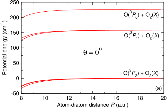
Figure 2: (a) Asymptotic PESs for the nine spin-orbit states O(³P_0,1,2) + O${}_{2}(X^{3}\Sigma^{-}_{g})$ at $r=r_{e}=2.282$ a.u. and $\theta$=0^∘. (b) Asymptotic PESs for the five lowest spin-orbit states correlated to O(³P₂) + O${}_{(}2X^{3}\Sigma^{-}_{g})$ at $r=r_{e}=2.282$ a.u. and $R=10$ a.u.. In (b) the dotted line refer to the ground state PES without fine-structure.

Inclusion of spin-orbit splitting lifts the degeneracy of the states and twenty-seven states arise from the interaction of O(${}^{3}P_{J_{a}}$) with O₂(X${}^{3}\Sigma^{-}_{g}$), which reduce to nine states if we neglect the O₂ fine-structure (Fig. 2(a)). The angular dependence of the five states correlated to the O(${}^{3}P_{2}$)+O₂(X${}^{3}\Sigma^{-}_{g}$) limit are displayed for $R=10$ a.u. on Fig. 2(b), where the influence of the spin-orbit interaction of O(${}^{3}P_{2}$) on the anisotropy of the PES is clearly visible.

III Asymptotic potential energy curves between O and O₂ in a given rovibrational level

III.1 Model

The calculations presented in this section are based on our previous work on Cs($6p\,{}^{2}P$)–Cs${}_{2}(^{1}\Sigma_{g}^{+},v_{d}=0,N_{d})$ lepers2010 ; lepers2011a ; lepers2011b ; lepers2011c performed in the context of ultracold gases. The main differences are that the present work deals (i) with a ground-state atom, and (ii) with a triplet molecule ($S_{d}=1$).

When an oxygen atom approaches a rovibrating O₂ molecule from large distances, the rotational levels of O₂ are coupled by the electric field induced by O. We focus on the derivation of one-dimensional long-range potential energy curves (PECs) for the O–O₂ complex depending on $R$, thus describing the interaction in the frame $xyz$ linked to the complex. In other words we leave out here the mutual rotation of O and O₂.

The quantities regarding the oxygen atom are expressed here in the fine-structure basis $|J_{a}M_{a}\rangle$ and are identical to those of Section II. To stress the differences with the fixed-geometry problem for the diatom, all the quantities $X$ that are averaged over O₂ vibrational wave functions are overlined ($\overline{X}$). Note that the effects of centrifugal distortion on those wave functions will be ignored.

III.1.1 Zeroth-order energies and state vectors

We consider that the O₂ molecule lies in its ground vibrational level $v_{d}=0$. In addition to the electronic quantum numbers $\Lambda_{d}=0$, $S_{d}=1$ and $\Sigma_{d}$ of O₂, we introduce the quantum numbers for the (electronic$+$nuclear) orbital angular momentum $N_{d}$, for the orbital$+$spin angular momentum $J_{d}$ ($\left|N_{d}-1\right|\leq J_{d}\leq N_{d}+1$), and the corresponding projections $M_{d}$, $M_{N_{d}}$ (and $M_{S_{d}}$ for $S_{d}$) on the $z$ axis. Here we limit our study to the ${}^{16}\textrm{O}_{2}$ isotopologue allowing for odd values of $N_{d}$ only vdavoird1987 . All the matrix elements will be given in the fine-structure basis $\left|(N_{d}S_{d})J_{d}M_{d}\right\rangle\equiv\left|N_{d}J_{d}M_{d}\right\rangle$, connected to the $\left|N_{d}M_{N_{d}}S_{d}M_{S_{d}}\right\rangle$ basis by

$$\left|N_{d}J_{d}M_{d}\right\rangle=\sum_{M_{N_{d}}M_{S_{d}}}C_{N_{d}M_{N_{d}}S_{d}M_{S_{d}}}^{J_{d}M_{d}}\left|N_{d}M_{N_{d}}S_{d}M_{S_{d}}\right\rangle,$$ (21)

where $C_{N_{d}M_{N_{d}}S_{d}M_{S_{d}}}^{J_{d}M_{d}}=\langle N_{d}M_{N_{d}}S_{d}M_{S_{d}}|J_{d}M_{d}\rangle$ denotes a Clebsch-Gordan coefficient.

In its ground electronic state, O₂ belongs to Hund’s case b, i.e. $N_{d}$ is considered as a good quantum number. The rotational spectrum is dominated by the free-rotator contribution $\overline{B}_{v_{d}}\mathbf{N}_{d}^{2}$, with $\overline{B}_{v_{d}=0}=\overline{B}_{0}=1.438$  cm^-1 vdavoird1987 . The matrix element of the spin-spin interaction (Eq. (4)) are expressed in the $|J_{d}M_{d}\rangle$ basis (see Sec. III of the supplementary material epaps )

$$\overline{E}_{SS} = \langle J_{d}M_{d}|\hat{H}_{SS}|J_{d}M_{d}\rangle$$ (26)

$$= \left(-1\right)^{1+J_{d}}\frac{2\sqrt{30}}{3}\left(2N_{d}+1\right)\overline{\lambda}_{0}$$

$$\times\left\{\begin{array}[]{ccc}N_{d}&1&J_{d}\\ 1&N_{d}&2\end{array}\right\}\left(\begin{array}[]{ccc}N_{d}&2&N_{d}\\ 0&0&0\end{array}\right)\,,$$

where the spin-spin coupling constant $\overline{\lambda}_{0}=\overline{\lambda}_{v_{d}=0}=1.983$ cm^-1 is taken from Ref. tinkham1955 . The spin-spin interaction results into the splitting of the fine-structure rotational levels $J_{d}$ inside a given manifold $N_{d}$. The spin-rotation interaction $\hat{H}_{SR}=\overline{\mu}_{v_{d}=0}\hat{\mathbf{N}}_{d}\cdot\hat{\mathbf{S}}_{d}$ is characterized by a coupling constant $\overline{\mu}_{v_{d}=0}=8.43\times 10^{-3}$ cm^-1 tinkham1955 much smaller than $\overline{\lambda}_{0}$, and will be neglected in what follows.

The zeroth-order energy $\overline{E}_{0}$ is the sum of the atomic spin-orbit, the molecular rigid-rotator and the spin-spin interactions

$$\overline{E}_{0}=\frac{A}{2}\left(J_{a}\left(J_{a}+1\right)-6\right)+\overline{B}_{0}\left(N_{d}\left(N_{d}+1\right)-2\right)+\overline{E}_{SS}\,,$$ (27)

corresponding to unperturbed state vectors $|\overline{\Psi}_{0}\rangle=\left|J_{a}M_{a}\right\rangle\left|N_{d}J_{d}M_{d}\right\rangle$. The origin of energies $\overline{E}_{0}=0$ is fixed to the O$(^{3}P_{2})$+O${}_{2}(v_{d}=0,N_{d}=1)$ dissociation limit.

III.1.2 First-order quadrupole-quadrupole interaction

The quadrupole moment matrix elements of the vibrating and rotating O₂ molecule is obtained by starting from Eq. (12) of Ref. lepers2011b written in the $|N_{d}M_{N_{d}}S_{d}M_{S_{d}}\rangle$ basis, and by applying the transformation to the fine-structure basis $|N_{d}J_{d}M_{d}\rangle$ (Eq.(21))

$$\langle v_{d}=0,N_{d}J_{d}M_{d}|\hat{Q}_{2}^{-m}|v_{d}=0,N^{\prime}_{d}J^{\prime}_{d}M^{\prime}_{d}\rangle = \left(-1\right)^{1+J_{d}+J_{d}^{\prime}-M_{d}^{\prime}}\overline{q}_{0}\sqrt{\left(2J_{d}+1\right)\left(2J_{d}^{\prime}+1\right)}$$ (35)

$$\times\sqrt{\left(2N_{d}+1\right)\left(2N_{d}^{\prime}+1\right)}\left(\begin{array}[]{ccc}N_{d}&2&N_{d}^{\prime}\\ 0&0&0\end{array}\right)$$

$$\times\left\{\begin{array}[]{ccc}N^{\prime}_{d}&1&J^{\prime}_{d}\\ J_{d}&2&N_{d}\end{array}\right\}\left(\begin{array}[]{ccc}J_{d}&2&J^{\prime}_{d}\\ -M_{d}&-m&M^{\prime}_{d}\end{array}\right)\,,$$

where we use the expansion of the product of three Clebsh-Gordan coefficients (see Eq. (2) of the supplementary material epaps ), and where

$$\overline{q}_{0}\equiv\overline{q}_{v_{d}=0}=\int_{0}^{+\infty}dr\left(\psi_{v_{d}=0}(r)\right)^{2}q(r)\,$$ (36)

is the quadrupole operator averaged over the vibrational wave function $\psi_{v_{d}=0}(r)$. Its value $\overline{q}_{0}=-0.2273$ a.u. is taken from Ref. lawson1997 . The properties of the 3-j and 6-j symbols impose that $N_{d}^{\prime}=N_{d},N_{d}\pm 2$ and $J_{d}^{\prime}=J_{d},J_{d}\pm 1,J_{d}\pm 2$.

The $R$-dependent quadrupole-quadrupole matrix element reads

$$\overline{E}_{\mathrm{elec}}^{\,J_{a}M_{a}J^{\prime}_{a}M^{\prime}_{a}N_{d}J_{d}M_{d}N^{\prime}_{d}J^{\prime}_{d}M^{\prime}_{d}}(v_{d}=0,R)$$ (37)

$$= \frac{1}{R^{5}}\sum_{m=-2}^{2}g_{m}(2,2)\langle J_{a}M_{a}|\hat{Q}_{2}^{m}|J^{\prime}_{a}M^{\prime}_{a}\rangle$$

$$\times\langle v_{d}=0,N_{d}J_{d}M_{d}|\hat{Q}_{2}^{-m}|v_{d}=0,N^{\prime}_{d}J^{\prime}_{d}M^{\prime}_{d}\rangle\,,$$

where $g_{m}(2,2)$ is given by Eq. (2). Note that the atomic quadrupole moment, expressed in the fine-structure basis, is related to the one in the $|M_{L_{a}}M_{S_{a}}\rangle$ basis (see Eq. (8)),

$$\langle J_{a}M_{a}|\hat{Q}_{2}^{m}|J^{\prime}_{a}M^{\prime}_{a}\rangle = \sum_{M_{L_{a}}M_{S_{a}}}\sum_{M^{\prime}_{L_{a}}M^{\prime}_{S_{a}}}C_{1M_{L_{a}}1M_{S_{a}}}^{J_{a}M_{a}}C_{1M^{\prime}_{L_{a}}1M^{\prime}_{S_{a}}}^{J^{\prime}_{a}M^{\prime}_{a}}$$ (38)

$$\times \delta_{M_{S_{a}}M^{\prime}_{S_{a}}}\langle 1M_{L_{a}}|\hat{Q}_{2}^{m}|1M^{\prime}_{L_{a}}\rangle\,.$$

III.1.3 Second-order dipole-dipole interaction

In order to calculate the dispersion term in $R^{-6}$, we use the approach of Refs. lepers2011a ; lepers2011b , adapted with the notations of the present paper. In the atomic and molecular fine-structure bases, the matrix elements associated with the second-order dipole-dipole interaction reads

$$\overline{E}_{\mathrm{disp}}^{\,J_{a}M_{a}J^{\prime}_{a}M^{\prime}_{a}N_{d}J_{d}M_{d}N^{\prime}_{d}J^{\prime}_{d}M^{\prime}_{d}}(R)$$ (39)

$$= -\frac{1}{2\pi R^{6}}\sum_{m,m^{\prime}=-1}^{1}g_{m}(1,1)g_{m^{\prime}}(1,1)$$

$$\times \int_{0}^{+\infty}d\omega\,{}^{J_{a}M_{a}J^{\prime}_{a}M^{\prime}_{a}}\alpha_{1m1m^{\prime}}(i\omega)$$

$$\times\,{}^{N_{d}J_{d}M_{d}N^{\prime}_{d}J^{\prime}_{d}M^{\prime}_{d}}\overline{\alpha}_{1-m1-m^{\prime}}(i\omega),$$

where ${}^{J_{a}M_{a}J^{\prime}_{a}M^{\prime}_{a}}\alpha_{1m1m^{\prime}}(i\omega)$ and ${}^{N_{d}J_{d}M_{d}N^{\prime}_{d}J^{\prime}_{d}M^{\prime}_{d}}\overline{\alpha}_{1-m1-m^{\prime}}(i\omega)$ are the uncoupled dipole polarizabilities at imaginary frequencies, for the atom and the molecule respectively. Note that these polarizabilities are related to the ones defined in Ref. lepers2011a according to ${}^{xx^{\prime}}\alpha_{1m1m^{\prime}}(i\omega)=[(-1)^{m}]{}^{xx^{\prime}}\alpha_{m,-m^{\prime}}^{M_{x}M_{x}^{\prime}}(i\omega)$, where $x$ stands for the set of atomic or molecular quantum numbers (see Ref. lepers2011a , Eqs. (13) and (14)). The polarizabilities of O expressed in the fine-structure basis reads

$${}^{J_{a}M_{a}J^{\prime}_{a}M^{\prime}_{a}}\alpha_{1m1m^{\prime}}(i\omega) = \sum_{M_{L_{a}}M_{S_{a}}}\sum_{M^{\prime}_{L_{a}}M^{\prime}_{S_{a}}}C_{1M_{L_{a}}1M_{S_{a}}}^{J_{a}M_{a}}C_{1M^{\prime}_{L_{a}}1M^{\prime}_{S_{a}}}^{J^{\prime}_{a}M^{\prime}_{a}}$$ (40)

$$\times \delta_{M_{S_{a}}M^{\prime}_{S_{a}}}\,{}^{M_{L_{a}}M^{\prime}_{L_{a}}}\alpha_{1m1m^{\prime}}(i\omega)\,.$$

where ${}^{M_{L_{a}}M^{\prime}_{L_{a}}}\alpha_{1m1m^{\prime}}(i\omega)$ are the polarizabilities in the $|M_{L_{a}}M_{S_{a}}\rangle$ basis (see Eqs. (13) and (17)).

For O₂, the polarizabilities ${}^{J_{d}M_{d}J^{\prime}_{d}M^{\prime}_{d}}\overline{\alpha}_{1m1m^{\prime}}$ are calculated in Sec. IV of the supplementary material epaps , starting from our previous work lepers2011a ; lepers2011b . We obtain finally

$${}^{N_{d}J_{d}M_{d}N^{\prime}_{d}J^{\prime}_{d}M^{\prime}_{d}}\overline{\alpha}_{1m1m^{\prime}}(i\omega) = \left(-1\right)^{m}\delta_{J_{d}J^{\prime}_{d}}\delta_{M_{d}M^{\prime}_{d}}\delta_{m,-m^{\prime}}\frac{\overline{\alpha}_{0}^{\parallel}(i\omega)+2\overline{\alpha}_{0}^{\bot}(i\omega)}{3}$$ (50)

$$+ \sqrt{\frac{10}{3}}\sqrt{\left(2N_{d}+1\right)\left(2N^{\prime}_{d}+1\right)\left(2J_{d}+1\right)\left(2J^{\prime}_{d}+1\right)}$$

$$\times\left(-1\right)^{1+J_{d}+J_{d}^{\prime}-M_{d}^{\prime}}\left\{\begin{array}[]{ccc}N^{\prime}_{d}&1&J^{\prime}_{d}\\ J_{d}&2&N_{d}\end{array}\right\}\left(\begin{array}[]{ccc}N_{d}&2&N^{\prime}_{d}\\ 0&0&0\end{array}\right)$$

$$\times\left(\overline{\alpha}_{0}^{\parallel}(i\omega)-\overline{\alpha}_{0}^{\bot}(i\omega)\right)$$

$$\times\left(\begin{array}[]{ccc}2&1&1\\ M^{\prime}_{d}-M_{d}&m&m^{\prime}\end{array}\right)\left(\begin{array}[]{ccc}J_{d}&2&J^{\prime}_{d}\\ -M_{d}&M_{d}-M^{\prime}_{d}&M^{\prime}_{d}\end{array}\right),$$

where $\overline{\alpha}_{0}^{\parallel}=\overline{\alpha}_{v_{d}=0}^{\parallel}$ and $\overline{\alpha}_{0}^{\bot}=\overline{\alpha}_{v_{d}=0}^{\bot}$ are the parallel and perpendicular polarizabilities of O₂ in its vibrational ground level. Equation (50) is a sum of two contributions: The first term, proportional to the so-called isotropic polarizability $(\overline{\alpha}_{0}^{\parallel}+2\overline{\alpha}_{0}^{\bot})/3$, is diagonal; the second term, which is proportional to the so-called anisotropic polarizability $\overline{\alpha}_{0}^{\parallel}-\overline{\alpha}_{0}^{\bot}$, couples the different angular-momentum projections $M_{d}$. The properties of the 3-j and 6-j symbols impose that $N_{d}^{\prime}=N_{d},N_{d}\pm 2$ and $J_{d}^{\prime}=J_{d},J_{d}\pm 1,J_{d}\pm 2$.

III.2 Asymptotic potential energy curves

The asymptotic PECs are obtained after diagonalizing the potential energy matrix with elements (where we omitted the label $v_{d}=0$ for simplicity)

$$\overline{E}_{\mathrm{tot}}^{\,J_{a}M_{a}J^{\prime}_{a}M^{\prime}_{a}N_{d}J_{d}M_{d}N^{\prime}_{d}J^{\prime}_{d}M^{\prime}_{d}}(R) = \delta_{J_{a}M_{a}}\delta_{J^{\prime}_{a}M^{\prime}_{a}}\delta_{J_{d}M_{d}}\delta_{J^{\prime}_{d}M^{\prime}_{d}}\overline{E}_{0}$$ (51)

$$+ \overline{E}_{\mathrm{elec}}^{\,J_{a}M_{a}J^{\prime}_{a}M^{\prime}_{a}N_{d}J_{d}M_{d}N^{\prime}_{d}J^{\prime}_{d}M^{\prime}_{d}}(R)$$

$$+ \overline{E}_{\mathrm{disp}}^{\,J_{a}M_{a}J^{\prime}_{a}M^{\prime}_{a}N_{d}J_{d}M_{d}N^{\prime}_{d}J^{\prime}_{d}M^{\prime}_{d}}(R)\,,$$

for different values of $R$, and within the subspace determined by each value of the total angular momentum $M=M_{a}+M_{d}$ on the $z$ axis dubernet1994 ; lepers2010 ; lepers2011a ; lepers2011b ; lepers2011c . For $M=0$, the eigenvectors of (51) are also characterized by a given reflection symmetry through any plane containing the $z$ axis. Following the expression of the reflection operator $\sigma_{xz}$ for two atoms (see for instance Eq. (3.11) of Ref. chang1967 ), we assign the $\pm$ symmetry to eigenvectors corresponding to the linear combinations $|M_{a},-M_{a}\rangle\pm(-1)^{L_{a}+J_{a}+N_{d}+J_{d}}|-M_{a}M_{a}\rangle$. On Figs. 3–6, we display long-range potential curves belonging to the $M=0^{+}$ symmetry. The curves belonging to other symmetries have the same appearance, except that some asymptotic channels may not be allowed for a given value of $M$, e.g. $J_{a}=J_{d}=0$ for $M=1$. All the curves are strongly attractive, due to the dominance of the attractive van der Waals term in the range of O–O₂ distances that we consider here (see Tables 3 and 4 for an illustration of this point).

Figure 3: Long-range potential energy curves for the interaction between ¹⁶O$(^{3}P_{2,1,0})$ and ¹⁶O₂($X^{3}\Sigma_{g}^{-},v_{d}=0,N_{d}=1,3,5$), as functions of their mutual separation $R$, for $M=0$ and the $(+)$ reflection symmetry.

As the spin-orbit splitting of O is much larger than the rotational splitting of O₂ (at least for the $N_{d}$ lowest levels), we see in Fig. 3 that the corresponding fine-structure PEC manifolds are almost decoupled from each other. This situation corresponds to Hund’s-like case ”1C” defined in dubernet1994 , also valid in the Cs*+Cs₂ system lepers2011c . For the sake of clarity, we have restricted our plot to the first three (odd-parity) rotational levels of ¹⁶O₂ ($N_{d}=1,3,5$), even if in principle all the rotational levels up to infinity should be included in the calculation (see a discussion about this point in lepers2011b ). However, even at the low-$R$ limit of our calculations, the different $N_{d}$ levels remain almost uncoupled. As an illustration, at $R=8$ a.u., the PECs of Figs. 3–5 conserve at least $95\%$ of their asymptotic $N_{d}$ character. In other words, in the range of O–O₂ distances that we consider, the oxygen molecule rotates almost freely.

Figure 4: Same as Fig. 3, but focused on the ${}^{3}P_{2}$ fine-structure level of ¹⁶O.

Figure 5: Same as Fig. 3, but focused on the ${}^{3}P_{2}$ fine-structure level of O, and the $N_{d}=1$ rotational level of ¹⁶O₂.

The PECs obtained for other O₂ isotopologues, not shown here, have similar features as Figs. 3–5. But caution has to be taken on which $N_{d}$ values are allowed. For ${}^{18}\textrm{O}_{2}$, the allowed $N_{d}$ values are the odd ones, whereas for ${}^{17}\textrm{O}_{2}$, the allowed values are the even/odd ones, if the total nuclear spin is odd/even. For mixed isotopologues, that is ${}^{16}\textrm{O}^{17}\textrm{O}$, ${}^{16}\textrm{O}^{18}\textrm{O}$ and ${}^{17}\textrm{O}^{18}\textrm{O}$, all values of $N_{d}$ are possible. But since the Hamiltonian of Eq. (51) conserves the parity of $N_{d}$, even and odd values can still be separated from each other.

Figure 6: The long-range potential curves of Fig. 5 (solid lines) dressed with a centrifugal term corresponding to a collisional partial wave $L=10$ for the ¹⁶O₂-¹⁶O system. Note that the $R$ axis is logarithmic.

In order to get an insight into the collisional dynamics between O and O₂, we have added to our curves a centrifugal term $L(L+1)/2\mu R^{2}$, where $L$ is the partial wave of the collision that we took equal to 10, and $\mu$ the reduced mass of the O–O₂ system (Fig. 6). This term competes with the attractive van der Waals interaction, and creates a centrifugal barrier of about 2 cm^-1, or about 3 Kelvin. This temperature being much lower than even the lowest temperatures of ozone samples, we can conclude that many partial waves should be included in a full quantum treatment of the O–O₂ collision.

IV Discussion: how do the two approaches connect to each other?

In the previous sections, we have calculated the matrix elements of the potential energy operator of the long-range interaction between ground state O and O₂, yielding its eigenvalues after diagonalization in the appropriate configuration subspace: either for fixed geometries of the O–O₂ complex leading to ($R$,$\theta$,$r\equiv r_{e}$)-dependent electronic PESs (Section II), or for a given rovibrational state of O₂ leading to $R$-dependent PECs (Section III). It is clear that those two adiabatic potential energy sets are not directly related to each other; instead, the matrix elements of the latter approach are obtained by averaging those of the former approach on the $r$ and $\theta$ coordinates of O₂, as briefly addressed in Ref. dubernet1994 . This is easily demonstrated on the matrix elements of the quadrupole-quadrupole interaction. Equation (35) shows that the ro-vibrationally averaged matrix element of the diatom quadrupole moment reads

$$\left\langle v_{d}N_{d}J_{d}M_{d}\left|\hat{Q}_{2}^{-m}\right|v_{d}N_{d}^{\prime}J_{d}^{\prime}M_{d}^{\prime}\right\rangle=\overline{q}_{v_{d}}\int_{0}^{\pi}d\theta\sin\theta\psi_{N_{d}J_{d}M_{d}}(\theta)d_{-m0}^{2}(\theta)\psi_{N_{d}^{\prime}J_{d}^{\prime}M_{d}^{\prime}}(\theta)\,,$$ (52)

where

$$\psi_{N_{d}J_{d}M_{d}}(\theta)=\sqrt{\frac{2N_{d}+1}{2}}\sum_{M_{N_{d}}M_{Ns}}\langle N_{d}M_{N_{d}}S_{d}M_{S_{d}}|J_{d}M_{d}\rangle d_{M_{N_{d}}0}^{N_{d}}(\theta)$$ (53)

is the angular part of the wave function of the fine-structure rotational level. We thus have

$$\overline{E}_{\mathrm{elec}}^{\,J_{a}M_{a}J^{\prime}_{a}M^{\prime}_{a}N_{d}J_{d}M_{d}N^{\prime}_{d}J^{\prime}_{d}M^{\prime}_{d}}(R)=\int_{0}^{+\infty}dr\left(\psi_{v_{d}}(r)\right)^{2}\int_{0}^{\pi}d\theta\sin\theta\psi_{N_{d}J_{d}M_{d}}(\theta)\psi_{N_{d}^{\prime}J_{d}^{\prime}M_{d}^{\prime}}(\theta)E_{\mathrm{elec}}^{\,J_{a}M_{a}J^{\prime}_{a}M^{\prime}_{a}}(R,r,\theta)\,.$$ (54)

The situation for the second-order dipole-dipole interaction is slightly more subtle. In Sec. V of the supplementary material epaps , we demonstrate that as far as the rotation of O₂ is concerned, the passage from one approach to the other is made by averaging $E_{\mathrm{disp}}$ over the rotational wave function $\psi_{N_{d}J_{d}M_{d}}(\theta)$, which can be schematically summarized as follows

$$d_{-\mathcal{M}0}^{\mathcal{L}_{d}}(\theta)\mathrm{\,[in\,}E_{\mathrm{disp}}\mathrm{]}\to\int_{0}^{\pi}d\theta\sin\theta\psi_{N_{d}J_{d}M_{d}}(\theta)d_{-\mathcal{M}0}^{\mathcal{L}_{d}}(\theta)\psi_{N_{d}^{\prime}J_{d}^{\prime}M_{d}^{\prime}}(\theta)\mathrm{\,[in\,}\overline{E}_{\mathrm{disp}}\mathrm{]}\,,$$ (55)

where $E_{\mathrm{disp}}=E_{\mathrm{disp}}^{J_{a}M_{a}J^{\prime}_{a}M^{\prime}_{a}}$ and $\overline{E}_{\mathrm{disp}}=\overline{E}_{\mathrm{disp}}^{\,J_{a}M_{a}J^{\prime}_{a}M^{\prime}_{a}N_{d}J_{d}M_{d}N^{\prime}_{d}J^{\prime}_{d}M^{\prime}_{d}}$ are given by Eqs. (9) and (39), respectively.

The drawback which can occur when taking in account the vibration of O₂ is illustrated by considering the static parallel electronic polarizability $\alpha^{\parallel}(\omega=0;r)$

$$\alpha^{\parallel}(\omega=0;r)=2\sum_{e\neq X}\frac{\mu_{Xe}^{2}(r)}{V_{e}(r)-V_{X}(r)}\,,$$ (56)

where $V_{X}(r)$ and $V_{e}(r)$ are the potential energy curves of the ${}^{3}\Sigma_{g}^{-}$ ground state and of the excited electronic states, respectively, and $\mu_{Xe}(r)$ the ($r$-dependent) transition dipole moment between states $X$ and $e$. Eq. (56) is a strict application of the Born-Oppenheimer approximation, i.e. the molecular response to an electric field is only due to the electrons. The most straightforward way to take into account the vibration of O₂ would be to average (56) over the vibrational wave function,

$$\langle\alpha^{\parallel}(r)\rangle_{v_{d}}=2\sum_{e\neq X}\int_{0}^{+\infty}dr\psi_{v_{d}}(r)\frac{\mu_{Xe}^{2}(r)}{V_{e}(r)-V_{X}(r)}\psi_{v_{d}}(r)\,.$$ (57)

However, one sees that Eq. (57) differs from the polarizability $\overline{\alpha}_{v_{d}}^{\parallel}$ associated with the vibrational level $v_{d}$, which reads

$$\overline{\alpha}_{v_{d}}^{\parallel}=2\sum_{e,v^{\prime}_{d}\neq X,v_{d}}\frac{\langle v^{\prime}_{d}|\mu_{Xe}(r)|v_{d}\rangle^{2}}{E_{ev^{\prime}_{d}}-E_{Xv_{d}}}\,,$$ (58)

where $E_{ev^{\prime}_{d}}$ and $E_{Xv_{d}}$ are the electronic and vibrational energy levels of the field-free molecule. Note that $v^{\prime}_{d}$ can also stand for a continuum state, in which case the discrete sum in Eq. (58) becomes an integral. As pointed out in Ref. bishop1990 , Eqs.(57) and (58) are identical if one neglects the diatom zero-point energy, i.e. $E_{Xv_{d}}=E_{X}(r=r_{e})$ and $E_{ev^{\prime}_{d}}=E_{e}(r=r_{e})$, where $r_{e}$ is the O₂ equilibrium distance in its ground state.

To check the validity of this approximation is appropriate for O₂, we have considered the two lowest excited $B^{3}\Sigma_{u}^{-}$ and $E^{3}\Sigma_{u}^{-}$ electronic states in the sums above (Fig. 7). The $X$ and $B$ PECs, as well as the transition dipole moment $\mu_{XB}(r)$ are taken from Refs. allison1986 ; friedman1990 . The PEC for the pure $E$ Rydberg state is taken from Ref. wang1987 , and we have extended it for $2.8a_{0}<r<3a_{0}$ by shifting down the experimental potential curve of O${}_{2}^{+}(X^{2}\Pi_{g})$ singh1966 . The transition dipole moment between $X$ and $E$ has been extracted from Ref. wang1987 . As described in Ref.spelsberg1998 , the $B$ and $E$ states exhibit an avoided crossing around 2.3$a_{0}$ close to the $X$ equilibrium distance $r_{e}$, due to a valence-Rydberg exchange of character. The $B$ state is steep and purely repulsive around $r_{e}$, while the minimum of the $E$ state is located at $r=2.25a_{0}$, namely close to $r_{e}$.

Figure 7: Potential energy curves of O₂: (a) for the $B^{3}\Sigma_{u}^{-}$ state (dashed lines) and the $E^{3}\Sigma_{u}^{-}$ state (dotted lines), (b) for the $X^{3}\Sigma_{g}^{-}$ state. (c) transition dipole moments: $B\leftarrow X$ (dashed lines), $E\leftarrow X$ (dotted lines). Between the two vertical lines, the wave-function of the $X,v_{d}=0$ level is more than half its maximum value.

The numerical values of Eqs.(56-58) obtained within this three-state model are presented in Table 5. The electronic polarizability of the $X$ state $\alpha^{\parallel}(r_{e})=$5.75 a.u. amounts for 40% of the total parallel polarizability kumar1996 . The three determinations are almost identical, despite the particular shape of the PECs. The partial contribution of each transition, ($B\leftarrow X$) and ($E\leftarrow X$) show a discrepancy between $\alpha^{\parallel}(r)$ on the one hand, and $\langle\alpha^{\parallel}(r)\rangle_{0}$ and $\overline{\alpha}_{0}^{\parallel}$ on the other hand, which is due to the sudden changes in potential curves and transition dipole moment within the spatial extension of the $X,v_{d}=0$ level. The fact that these differences compensate each other is due to the exchange in character between the two excited electronic states. In contrast, inside each electronic transition, $\langle\alpha^{\parallel}(r)\rangle_{v_{d}}$ and $\overline{\alpha}_{v_{d}}^{\parallel}$ are always nearly equal. On a physical point of view, it confirms that the response to an external electric field is, to a very large extent, due to the electrons, and not to the nuclei, which justifies the use of the Born-Oppenheimer approximation.

Table 5: Static parallel polarizability of O₂ calculated with three electronic states (see text): $\alpha^{\parallel}(r_{e})$ is purely electronic polarizability, evaluated at the O₂ equilibrium distance (see Eq. (56)), $\langle\alpha^{\parallel}(r)\rangle_{v_{d}=0}$ is the $r$-dependent electronic polarizability averaged over the ground-level vibrational wave function (see Eq. (57)), and $\overline{\alpha}_{v_{d}=0}^{\parallel}$ is purely vibrational (see Eq. (58)). We present the contribution of individual electronic transitions, $B\leftarrow X$ and $E\leftarrow X$, to the polarizability.

Transition	$\alpha^{\parallel}(r_{e})$	$\langle\alpha^{\parallel}(r)\rangle_{v_{d}=0}$	$\overline{\alpha}_{v_{d}=0}^{\parallel}$
$B\leftarrow X$	5.47	5.16	5.15
$E\leftarrow X$	0.29	0.63	0.63
Total	5.75	5.79	5.78

Our result tends to prove that the vibrational part of the energy (see Eq. (58)) can be neglected, whether the excited state PEC has a potential well or is purely repulsive. In the first situation, which corresponds to the $E\leftarrow X$ transition, the ground vibrational level $v_{d}=0$ has significant Franck-Condon factor (higher than $10^{-4}$) with the $E$ vibrational levels ranging from $v=0$ to 4. The vibrational energies (with respect to the corresponding minimum electronic energies) associated with $X,v_{d}=0$ and $E,v=4$ are 791 cm^-1 and 10300 cm^-1 respectively. So they are very small compared to the difference in electronic energy, which equals to 80000 cm^-1 at $r=r_{e}$. The ground vibrational level $v_{d}=0$ significantly overlaps with continuum states of the purely repulsive $B$ state whose classical turning point is located in the Franck-Condon region. This turning point region is precisely where the vibrational, i.e. kinetic part of the energy is small. In the present case, we only have the O₂ polarizabilities at the equilibrium distance $r_{e}$. In consequence, we assumed that the relationship between the fixed-geometries and the ro-vibrationally averaged approach, given for $E_{\mathrm{elec}}$ in Eq. (54), can be extended to $E_{\mathrm{disp}}$, and hence for $E_{\mathrm{tot}}$, within a good approximation.

V Conclusion

In this article, we have characterized the potential energy surfaces (PESs) of the ozone molecule at large distances, where O and O₂ weakly interact with each other, using two different approaches. Our calculations are based on the multipolar expansion of the electrostatic potential energy, which is expressed in terms of the electric properties of O and O₂.

Firstly, we have calculated the 27 asymptotic electronic PESs correlated to the O$(^{3}P)$–O${}_{2}(X^{3}\Sigma_{g}^{-})$ dissociation limit including spin-orbit couplings. All the PESs are found attractive due to the dominant isotropic van der Waals interaction. For all spin-orbit states, the minimum energy is observed for a linear configuration of the three oxygen atoms. These long-range PESs can readily be connected at short distances to the most recent ones obtained by high-level ab initio calculations dawes2011 , in order to derive global PESs for all values of the chosen internal coordinates. The overlap of the long-range and ab initio PESs on a large enough range of distances in the region of the LeRoy radius should avoid the tedious calculation of higher order terms in the multipolar expansion.

Secondly, we have considered the interaction between an O${}_{2}(X^{3}\Sigma_{g}^{-})$ molecule in a given spin-orbit state, vibrating in the ground level and rotating in a low level and an O$(^{3}P)$ atom. We obtained one-dimensional potential energy curves (PECs) dominated by the isotropic van der Waals interaction. They are nearly parallel, which indicates that, when O and O₂ approach each other, the rotation of O₂ is only weakly hindered by the presence of O at distances larger than the LeRoy radius. It is worthwhile to note that this hypothesis is generally assumed in models characterizing the transition state, which is located at smaller distances, in the O+O₂ exchange reaction hathorn2000 ; gao2001 ; gao2002 . However, such an hypothesis of weakly hindered rotation is not always appropriate, as demonstrated for instance in the long-range interaction between a cesium atom and a ground state Cs₂ molecule lepers2011c .

The one-dimensional PEC above can be smoothly matched to an arbitrary potential curve below the LeRoy radius so that vibrational energies and wavefunctions (along the O–O₂ axis) can be calculated in the frame attached to the trimer (i.e. neglecting the mutual rotation of O and O₂. They will be of relevance for estimating the density of vibrational levels of the O–O₂ system close to the dissociation limit, namely with binding energy smaller than the remaining potential energy $V(R_{LR})\approx 30$ cm^-1 around the LeRoy radius. Such wavefunctions will be mostly concentrated at large distances, since the potential energy around the O₃ global minimum is by far larger than $V(R_{LR})$. Once experimental energies are available near the dissociation limit, one could tune the potential energy in the inner zone in order to match the calculated energies to the observed one, and thus characterize the related energy levels with quantum numbers of the O–O₂ system.

Furthermore, such PECs could be of interest for the study of O–O₂ collisions in the cold ($T\lesssim 1$ K) or ultracold ($T\lesssim 1$ mK) regimes. Several theoretical studies already aimed at modeling collisions involving oxygen avdeenkov2001 ; volpi2002 ; tilford2004 ; perez-rios2009 ; perez-rios2011 , while several experimental investigations suggested possible ways to create beams of cold atomic or molecular oxygen patterson2007 ; narevicius2008 ; bucicov2008 . In particular, we can expect such collisions to exhibit rotational unconventional isotopic effects. If the difference in rotational energy compensates the difference in vibrational zero-point energy, we obtain two quasi-degenerate channels of different isotopologues. In addition, the nuclear-spin symmetry can also play an important part in the rotational isotopic effects, as it forbids some rotational levels. For example, the channels ${}^{17}\mathrm{O}+^{16}\mathrm{O}_{2}(N_{d}=3)$ and ${}^{16}\mathrm{O}+^{16}\mathrm{O}^{17}\mathrm{O}(N_{d}=4)$ on the one hand, and ${}^{18}\mathrm{O}+^{17}\mathrm{O}^{18}\mathrm{O}(N_{d}=3)$ and ${}^{17}\mathrm{O}+^{18}\mathrm{O}_{2}(N_{d}=4)$ on the other hand, are only separated by 0.2 cm^-1; but the second situation is not allowed, as ${}^{18}\mathrm{O}_{2}$ has no even rotational levels.

It is worthwhile to mention that in contrast with similar studies devoted to low energy atom exchange reactions in atom-diatom systems (for instance Al+O₂ reignier1998 , C+OH jorfi2010 , or O+OH stoecklin2012 ), the adiabatic capture centrifugal theory levine1987 conducted in the sudden approximation (ACCSA) clary1984 relying on the unique knowledge of the long-range asymptotic ground state potential energy of the atom-diatom system cannot be used in the ozone case, due to the presence of the transition state playing a role at distances lower than the LeRoy radius, and thus beyond the validity of the present approach. A calculation within this model would undoubtedly lead to an overestimation of the atom exchange rate.

References

• (1) R. Schinke, S. Y. Grebenshchikov, M. V. Ivanov, and P. Fleurat-Lessard. Dynamical studies of the ozone isotope effect: A status report. Annu. Rev. Phys. Chem., 57:625–661, 2006.
• (2) M.H. Thiemens and J.E. Heidenreich. The mass-independent fractionation of oxygen: A novel isotope effect and its possible cosmochemical implications. Science, 219:1073, 1983.
• (3) K. Mauersberger. Ozone isotope measurements in the stratosphere. Geophys. Res. Lett., 14:80–83, 1987.
• (4) S.M. Anderson, D. Hülsebusch, and K. Mauersberger. Surprising rate coefficients for four isotopic variants of o$+$o${}_{2}+$m. J. Chem. Phys., 107:5385–5392, 1997.
• (5) C. Janssen, J. Guenther, K. Mauersberger, and D. Krankowsky. Kinetic origin of the ozone isotope effect: a critical analysis of enrichments and rate coefficients. Phys. Chem. Chem. Phys., 3(21):4718–4721, 2001.
• (6) K. Mauersberger, D. Krankowsky, C. Janssen, and R. Schinke. Assessment of the ozone isotope effect. Adv. At. Mol. Opt. Phys., 50:1–54, 2005.
• (7) C. Janssen, J. Guenther, D. Krankowsky, and K. Mauersberger. Relative formation rates of 50o3 and 52o3 in 16o–18o mixtures. J. Chem. Phys., 111:7179–7182, 1999.
• (8) Y.Q. Gao and R.A. Marcus. Strange and unconventional isotope effects in ozone formation. Science, 293:259–263, 2001.
• (9) Y.Q. Gao and R.A. Marcus. On the theory of the strange and unconventional isotopic effects in ozone formation. J. Chem. Phys., 116:137–154, 2002.
• (10) S.Y. Grebenshchikov, R. Schinke, P. Fleurat-Lessard, and M. Joyeux. van der Waals states in ozone and their influence on the threshold spectrum of O ($x^{1}a_{1}$). i. bound states. J. Chem. Phys., 119:6512, 2003.
• (11) D. Babikov. Entrance channel localized states in ozone: Possible application to helium nanodroplet isolation spectroscopy. J. Chem. Phys., 119:6554, 2003.
• (12) H.S. Lee and J.C. Light. Vibrational energy levels of ozone up to dissociation revisited. J. Chem. Phys., 120:5859, 2004.
• (13) D. Babikov, B.K. Kendrick, R.B. Walker, R.T. Pack, P. Fleurat-Lesard, and R. Schinke. Metastable states of ozone calculated on an accurate potential energy surface. J. Chem. Phys., 118:6298–6308, 2003.
• (14) S. Y. Grebenshchikov and R. Schinke. Towards quantum mechanical description of the unconventional mass-dependent isotope effect in ozone: Resonance recombination in the strong collision approximation. J. Chem. Phy., 131:181103, 2009.
• (15) P. Fleurat-Lessard, S.Y. Grebenshchikov, R. Siebert, R. Schinke, and N. Halberstadt. Theoretical investigation of the temperature dependence of the o+o2 exchange reaction. J. Chem. Phys., 118:610, 2003.
• (16) M.V. Ivanov and D. Babikov. Efficient quantum-classical method for computing thermal rate constant of recombination: Application to ozone formation. J. Chem. Phys., 136:184304, 2012.
• (17) R. Siebert, R. Schinke, and M. Bittererová. Spectroscopy of ozone at the dissociation threshold: Quantum calculations of bound and resonance states on a new global potential energy surface. Phys. Chem. Chem. Phys., 3:1795–1798, 2001.
• (18) R. Siebert, P. Fleurat-Lessard, R. Schinke, M. Bittererová, and S.C. Farantos. The vibrational energies of ozone up to the dissociation threshold: Dynamics calculations on an accurate potential energy surface. J. Chem. Phys., 116:9749–9767, 2002.
• (19) P. Rosmus, P. Palmieri, and R. Schinke. The asymptotic region of the potential energy surfaces relevant for the o $(p)+$o${}_{2}(x^{3}\sigma_{g}^{-}$)$\rightleftharpoons$o3 reaction. J. Chem. Phys., 117:4871–4877, 2002.
• (20) F. Holka, P.G. Szalay, T. Müller, and V.G. Tyuterev. Toward an improved ground state potential energy surface of ozone. J. Phys. Chem. A, 114:9927–9935, 2010.
• (21) R. Dawes, P. Lolur, J. Ma, and H. Guo. Communication: Highly accurate ozone formation potential and implications for kinetics. J. Chem. Phys., 135:081102, 2011.
• (22) M. Tashiro and R. Schinke. The effect of spin–orbit coupling in complex forming o(${}^{3}p$)+o2 collisions. J. Chem. Phys., 119:10186, 2003.
• (23) B. Bussery-Honvault, F. Dayou, and A. Zanchet. Long-range multipolar potentials of the 18 spin-orbit states arising from the C (${}^{3}{P}$) + OH(X${}^{2}{\Pi}$) interaction. J. Chem. Phys., 129:234302, 2008.
• (24) B. Bussery-Honvault and F. Dayou. Si (${}^{3}{P}$) + OH (X${}^{2}{\Pi}$) interaction: Long-range multipolar potentials of the eighteen spin-orbit states. J. Phys. Chem. A, 113(52):14961, 2009.
• (25) M. Lepers, O. Dulieu, and V. Kokoouline. Photoassociation of a cold atom-molecule pair: long-range quadrupole-quadrupole interactions. Phys. Rev. A, 82:042711, 2010.
• (26) R.J. LeRoy. Long-range potential coefficients from RKR turning points: $C_{6}$ and $C_{8}$ for $B(^{3}{\Pi}_{{Ou}^{+}})$-state Cl2, Br2, and I2. Can. J. Phys., 52:246, 1974.
• (27) M. Bartolomei, E. Carmona-Novillo, J. Campos-Martinez M.I. Hernandez, and R. Hernandez-Lamoneda. J. Comput. Chem., 32:279–290, 2010.
• (28) M. Tinkham and M. W. P. Strandberg. Theory of the fine structure of the molecular oxygen ground state. Phys. Rev., 97:937–951, 1955.
• (29) D. A. Varshalovich, A. N. Moskalev, and V. K. Khersonskii. Quantum theory of angular momentum. Leningrad, 1988.
• (30) D. Spelsberg, T. Lorenz, and W. Meyer. Dynamic multipole polarizabilities and long range interaction coefficients for the systems H, Li, Na, K, He, H-, H2, Li2, Na2, and K2. J. Chem. Phys., 99:7845, 1993.
• (31) P.W. Langhoff and M. Karplus. Padé approximants for two-and three-body dipole dispersion interactions. J. Chem. Phys., 53:233–250, 1970.
• (32) EPAPS no. NNN.
• (33) T. Stoecklin, B. Bussery-Honvault, P. Honvault, and F. Dayou. Asymptotic potentials and rate constants in the adiabatic capture centrifugal sudden approximation for X + OH$(X^{2}\Pi)\to$ OX + H$(^{2}S)$ reactions where X = O$(^{3}P)$, S$(^{3}P)$ or N$(^{4}S)$. Comp. Theor. Chem., 990:39–46, 2012.
• (34) G.L. Gutsev, P. Jena, and R.J. Bartlett. Chem. Phys. Lett., 291:547, 1998.
• (35) A.K. Das and A.J. Thakkar. J. Phys. B, 31:2215, 1998.
• (36) M. Medved, P.W. Fowler, and J.M. Hutson. Mol. Phys., 98:453, 2000.
• (37) D. B. Lawson and J. F. Harrison. Distance dependence and spatial distribution of the molecular quadrupole moments of H2, N2, O2, and F2. J. Phys. Chem. A, 101(26):4781–4792, 1997.
• (38) A. Kumar, W. J. Meath, P. Bündgen, and A. J. Thakkar. Reliable anisotropic dipole properties, and dispersion energy coefficients, for o evaluated using constrained dipole oscillator strength techniques. J. Chem. Phys., 105:4927–4937, 1996.
• (39) D.A. Dummur A.D. Buckingham, R.L. Disch. J. Am. Chem. Soc., 90:3104, 1968.
• (40) M.A. Buldakov, I.I. Ippolitov, B.V. Korolev, I.I. Matrosov, A.E. Cheglokov, V.N. Chrerepanov, Yu.S. Makushkin, and O.N. Ulenikov. Spectrochim. Acta A, 52:995, 1996.
• (41) E. Cohen and Birnbaum G.J. J. Chem. Phys., 66:2443, 1977.
• (42) N.J. Bridge and A.D. Buckingham. Proc. R Soc. London Ser. A, 295:334, 1966.
• (43) M. Lepers, R. Vexiau, N. Bouloufa, O. Dulieu, and V. Kokoouline. Photoassociation of a cold atom-molecule pair: second-order perturbation approach. Phys. Rev. A, 83:042707, 2011.
• (44) M. Lepers and O. Dulieu. Ultracold atom-dimer long-range interactions beyond the $1/r^{n}$ expansion. Eur. Phys. J. D, 165:113–123, 2011.
• (45) M. Lepers and O. Dulieu. Long-range interactions between ultracold atoms and molecules including atomic spin-orbit. Phys. Chem. Chem. Phys., 13:19106–19113, 2011.
• (46) A. Van der Avoird and G. Brocks. The O2-O2 dimer: magnetic coupling and spectrum. J. Chem. Phys, 87:5346–5360, 1987.
• (47) M.-L. Dubernet and J. M. Hutson. Atom-molecule van der Waals complexes containing open-shell atoms. i. general theory and bending levels. J. Chem. Phys., 101:1939–1958, 1994.
• (48) T. Y. Chang. Moderately long-range interatomic forces. Rev. Mod. Phys., 39(4):911–942, 1967.
• (49) D. M. Bishop. Molecular vibrational and rotational motion in static and dynamic electric fields. Rev. Mod. Phys., 62(2):343–374, 1990.
• (50) A.C. Allison, S.L. Guberman, and A. Dalgarno. A model of the Schumann-Runge continuum of O2. J. Geophys. Res., 91(A9):10193–10, 1986.
• (51) R.S. Friedman. Oscillator strengths of the schumann-runge bands of isotopic oxygen molecules. J. Quant. Spec. Rad. Trans., 43:225–238, 1990.
• (52) J. Wang, D.G. McCoy, A.J. Blake, and L. Torop. Effects of the close approach of potential curves in photoabsorption by diatomic molecules–ii. temperature dependence of the O2 cross section in the region 130-160 nm. J. Quant. Spec. Rad. Trans., 38:19–27, 1987.
• (53) R.B. Singh and D.K. Rai. Potential-energy curves for O${}_{2}^{+}+$, N${}_{2}^{+}$, and CO+. J. Mol. Spec., 19:424–434, 1966.
• (54) D. Spelsberg and W. Meyer. Ab initio dynamic dipole polarizabilities for O2, its photoabsorption spectrum in the schumann-runge region, and long-range interaction coefficients for its dimer. J. Chem. Phys., 109:9802–9810, 1998.
• (55) B.C. Hathorn and R.A. Marcus. An intramolecular theory of the mass-independent isotope effect for ozone. ii. numerical implementation at low pressures using a loose transition state. J. Chem. Phys., 113:9497–9509, 2000.
• (56) A. V. Avdeenkov and J. L. Bohn. Ultracold collisions of oxygen molecules. Phys. Rev. A, 64:052703, 2001.
• (57) A. Volpi and J.L. Bohn. Magnetic-field effects in ultracold molecular collisions. Phys. Rev. A, 65:052712, 2002.
• (58) K. Tilford, M. Hoster, P.M. Florian, and R.C. Forrey. Cold collisions involving rotationally hot oxygen molecules. Phys. Rev. A, 69:052705, 2004.
• (59) J. Pérez-Ríos, M. Bartolomei, J. Campos-Martínez, M.I. Hernández, and R. Hernández-Lamoneda. Quantum-mechanical study of the collision dynamics of $\mathrm{O}_{2}(^{3}{\Sigma}_{g}^{-})+\mathrm{O}_{2}(^{3}{\Sigma}_{g}^{-})$ on a new ab initio potential energy surface. J. Phys. Chem. A, 113:14952, 2009.
• (60) J. Pérez-Ríos, J. Campos-Martínez, and M.I. Hernández. Ultracold O2 + O2 collisions in a magnetic field: On the role of the potential energy surface. J. Chem. Phys., 134:124310, 2011.
• (61) D. Patterson and J.M. Doyle. Bright, guided molecular beam with hydrodynamic enhancement. J. Chem. Phys., 126:154307, 2007.
• (62) E. Narevicius, A. Libson, C.G. Parthey, I. Chavez, J. Narevicius, U. Even, and M.G. Raizen. Stopping supersonic oxygen with a series of pulsed electromagnetic coils: A molecular coilgun. Phys. Rev. A, 77:051401, 2008.
• (63) O. Bucicov, M. Nowak, S. Jung, G. Meijer, E. Tiemann, and C. Lisdat. Cold SO2 molecules by Stark deceleration. Eur. Phys. J. D, 46:463, 2008.
• (64) D. Reignier, T. Stoecklin, S.D. Le Picard, A. Canosa, and B.R. Rowe. Rate constant calculations for atom–diatom reaction involving an open-shell atom and a molecule in a $\sigma$ electronic state application to the reaction Al(${}^{2}P_{1/2,3/2}$)+O${}_{2}(X^{3}\Sigma_{g}^{-})\to$ AlO($X^{2}\Sigma^{+}$)+O$(^{3}P_{2,1,0})$. J. Chem. Soc., Faraday Trans., 94(12):1681–1686, 1998.
• (65) M. Jorfi, B. Bussery-Honvault, P. Honvault, T. Stoecklin, P. Larrégaray, and P. Halvick. Theoretical sensitivity of the C(${}^{3}P$)+OH($X^{2}\Pi$)$\to$CO($X^{1}\Sigma^{+}$)+H(${}^{2}S$) rate constant: The role of the long-range potential. J. Phys. Chem. A, 114(28):7494–7499, 2010.
• (66) R.D. Levine and R.B. Bernstein. Molecular Reaction Dynamics and Chemical Reactivity. Oxford University Press, 1987.
• (67) D.C. Clary. Rates of chemical reactions dominated by long-range intermolecular forces. Mol. Phys., 53(1):3–21, 1984.