Tools for Astrophysics: MESA and NuGrid

Abstract:

These notes provide a tutorial for those who want to use the state-of-the-art stellar evolution code MESA and post-processing nucleosyntheis tools of NuGrid. As an example, an application of MESA and NuGrid tools for simulations of a nova outburst and associated nucleosynthesis occurring on a $1.3\,M_{\odot}$ ONe white dwarf is presented.

1 What Are These Tools For?

MESA is a collection of Fortran-95 Modules for Experiments in Stellar Astrophysics. Its main module star can be used for one-dimensional stellar evolution simulations of almost any kind. For instance, it can compute without any interruption the evolution of a solar-type star from the pre-MS phase through the He-core flash and thermal pulses on the AGB towards white-dwarf cooling. The code works well for low, intermediate and high mass stars. Other modules provide star with state-of-the-art numerical algorithms, e.g. for adaptive mesh refinement and timestep control, atmospheric boundary conditions, and modern input physics (see Marco Pignatari’s tutorial on MESA/NuGrid physics packages).

NuGrid tools include codes and data enabling large-scale post-processing nucleosynthesis computations. These can be done either at one Lagrangian coordinate (with the one-zone code PPN), in which case changes of $T$ and $\rho$ with time at a chosen mass zone (the so-called “trajectory”) have to be provided, or for an entire star (with the multi-zone code MPPNP), in which case $T$ and $\rho$ have to be given as functions of $M_{r}$ for each evolutionary model (“cycle”).

The MESA star has an option to output an evolutionary sequence of stellar models in a compressed format readable by the NuGrid MPPNP code. This interface allows to run star with a small reaction network, sufficient to properly take into account the nuclear energy generation rate, followed by an MPPNP run that can use stellar models prepared by star as a background for detailed nucleosynthesis computations.

The star code uses multi-threading to speed up its execution on multiple CPU cores, while MPPNP uses MPI to run in parallel on multiple CPUs.

2 What Should You Know if You Want to Use These Tools?

I would recommend first to read the MESA and NuGrid manifestos that can be found on their websites, http://mesa.sourceforge.net/ and www.nugridstars.org. These documents describe important “terms and conditions” (actually, a sort of fair-play rules) for accessing and using the tools.

MESA is free for download from its website that also gives some information on how to install and run the code. Its technical details, physical assumptions, and unique modeling capabilities are reported and copiously illustrated in the MESA main “instrument” paper [2].

To be successfully compiled and executed, MESA needs several libraries to be installed on your Linux or MAC computer. In particular, MESA will require a recent version of ifort or gfortran compiler, linear algebra BLAS and LAPACK libraries, version-5 Hierarchical Data Format (HDF5) library, PGPLOT graphics library, ndiff fuzzy comparison tool, and SE library from the NuGrid project. You can find, download, and install them on your computer separately or, as an alternative, you can use a unified software development kit MESA SDK put together by Rick Townsend on the website www.astro.wisc.edu/$\sim$townsend that also explains how to build MESA. The most important next step is to correctly specify MESA installation parameters in the file mesa/utils/makefile_header. It contains step-by-step instructions that help to choose right options for the parameters. A special version of this file called makefile_header.mesasdk can be used by those who decided to take advantage of the MESA SDK kit.

To join the NuGrid collaboration and get an access to the NuGrid tools, you should send an email message expressing your interest to one of its active members, e.g. Marco Pignatari (mpignatari@gmail.com), Gabriel Rockefeller (gaber@lanl.gov), or Falk Herwig (fherwig@uvic.ca).

3 How to Run MESA Star?

During its installation, MESA conducts some tests. If results of these tests are correct, MESA reports about its successful installation, and it is now ready for use. The main working directory for running MESA star is mesa/star/work. It is a good idea to copy this template directory elsewhere. Then, at its new location, you should first change the directory path names that are assigned to the string variables mesa_data_dir and MESA_DIR at the tops of the files work/inlist_project and work/make/makefile, respectively. These changes will let your copy of the work directory know where the other MESA modules are located. After that, you should type ./mk in your work directory to make the code, followed by the command ./rn that launches the MESA star. As a result, the evolution of a star with predefined parameters will be calculated with a lot of various text and graphics output data sent to a number of files and popped-up windows.

In order to set up parameters for your own MESA star run, you have to use an inlist file or the inlist_project file, if the latter is read by the former. It contains three Fortran-95 parameter namelists: star_job, controls, and pgstar. Roughly speaking, the first namelist allows you to “build” your own stellar evolution code by specifying where an initial model is to be taken, what data from computed models you want to be extracted and saved in files, what input physics, in particular a MESA standard or your own customized nuclear network should be used, and other global parameters. In the second namelist, you assign values to parameters that are specific for an individual run, such as the initial chemical composition and mass of the star, conditions to stop the simulations, prescriptions for mass gain or loss at different evolutionary phases, a criterion for convective instability (Schwarzschild or Ledoux), and others. The controls namelist is also the place where you can add some non-standard physical assumptions to your stellar evolution simulations. At present, these include element diffusion, semiconvection and convective overshooting, as well as thermohaline, rotational and magnetic mixing. Finally, the third namelist customizes the graphics output.

The section “how to use MESA star” on the MESA website provides more details on setting up the parameters in the inlist. Although MESA star has a too large number of parameters to comprehend, all of them already have reasonable default values with which standard stellar evolution simulations can be done. The full lists of the star_job, controls, and pgstar parameters with their default values can be found in the files run_star_defaults.dek, star_defaults.dek, and pgstar_defaults.dek located in the directory mesa/star/ public.

A few words of caution are necessary for those who want to experiment with the MESA non-standard physical assumptions. It is your responsibility to verify that a set of inlist parameters that you choose will result in correct modeling of the corresponding physical process. It is a matter of fact that non-standard additions to the MESA star are made on requests of its active and potential users who may not thoroughly test them afterwards. Sometimes, an option that worked in a previous release of MESA may not be available or produces a different result in its newer version. This can happen if the addition is considered non-standard, and therefore not included in MESA regression testing. The best way to solve such a problem is to contact a person who has already used the non-standard physical assumption you are interested in and ask for advice. For this, you can use the MESA-users mailing list (http://lists.sourceforge.net/lists/listinfo/MESA-users/) or try the new MESA-user forum (http://mesastar.org/).

4 Application of MESA and NuGrid Tools for Simulations of Classical Nova Outbursts and Nucleosynthesis

If you want to reproduce someone else’s stellar evolution simulations with MESA, you need to have a copy of the inlist file and know the version of the MESA package with which the simulations were run. If the inlist reads other project inlists or non-standard files specifying the initial model and its chemical composition, nuclear network, and output data lists, you will also need these. MESA itself has a special directory /mesa/star/test_suite that contains examples of a large number of its possible applications. You can use one of these tests, that best suits your problem, as a starting point for its solution.

Classical novae are the results of thermonuclear explosions of hydrogen occurring on the surfaces of white dwarfs (WDs) that accrete H-rich material from their low-mass MS binary companions. In our MESA nova simulations, we have used inlists of two relevant test_suite cases:

• make_co_wd combines some “stellar engineering” tricks into a procedure that creates CO WD models from a range of initial masses,

• wd2 demonstrates the use of parameters that control accretion, as well as mass ejection options available for nova calculations.

Our extended nuclear network nova_ext.net includes 48 isotopes from H to ³⁰Si coupled by 120 reactions. The initial stellar models are the $1.0\,M_{\odot}$ and $1.15\,M_{\odot}$ CO WDs, and $1.15\,M_{\odot}$ and $1.3\,M_{\odot}$ ONe WDs. They have been prepared with inlists similar to the one in the directory make_co_wd.

Nova outbursts become stronger when WD’s mass increases, while its initial central temperature and the accretion rate decrease, the latter being limited by the range $10^{-11}\,M_{\odot}/\mbox{yr}\leq\dot{M}\leq 10^{-9}\,M_{\odot}/\mbox{yr}$ for classical novae. The observed enrichment of the ejecta of novae in heavy elements (C, N, O, and Ne) is believed to be a signature of mixing between the accreted envelope and WD. Like in most other 1D nova simulations, we do not model this mixing explicitly but, instead, assume that the WD already accretes a pre-enriched mixture of equal amounts of its core and solar-composition materials.

As a representative case demonstrating the application of MESA and NuGrid tools for simulations of nova outbursts and nucleosynthesis, we have chosen our model of a nova occurring on the $1.3\,M_{\odot}$ ONe WD with the initial central temperature $T_{\rm WD}=12$ MK and accretion rate $\dot{M}=2\times 10^{-10}\,M_{\odot}$/yr. Its evolutionary track is plotted in Fig. 1 (the blue curve in the left panel) from the start of accretion till the star has expanded to several solar radii as a result of explosion (the dashed black lines are the loci of constant $R$). The three right panels show the internal profiles of $T$ and $\rho$ (upper), mass fractions of some isotopes (middle), and temperature gradients (logarithmic and with respect to pressure) (lower) in the envelope of a model (the red star symbol in the left panel) in which the maximum temperature has reached its peak value, $T_{\rm max}\approx 355$ MK. In order to reproduce these computations (with the version 3611 of MESA), you will need their corresponding inlists, the initial WD model (ne_wd_1.3_12_mixed.mod), the chemical composition of the accreted envelope (ne_nova_1.3_mixed_comp), the nuclear networks nova_ext.net and nova.net, the latter having a shorter list of isotopes with which the WD models have been generated, and the file my_log_columns.list specifying the output data for each model. You will also have to use our modified fortran subroutine run_star_extras.f that should replace its standard copy in the directory work/src. All these files can be downloaded from the webpage http://astrowww.phys.uvic.ca/$\sim$dpa/MESA_NuGrid_Tutorial.html.

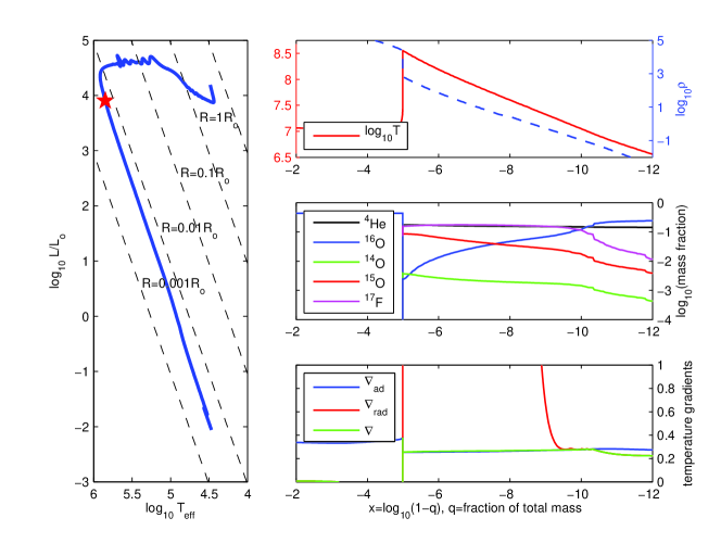
Figure 1: The results of our MESA simulations of the nova outburst occurring on the $1.3\,M_{\odot}$ ONe WD with the initial central temperature 12 MK and accretion rate $2\times 10^{-10}\,M_{\odot}/\mbox{yr}$. It is assumed that the WD accretes a pre-enriched mixture of equal amounts of WD’s core and solar-composition materials. Left panel: the evolutionary track (the blue curve) and location of the model with the peak maximum temperature at the base of the H-rich envelope (the red star symbol). The three right panels show the internal profiles of $T$ and $\rho$ (upper), mass fractions of some isotopes (middle), and temperature gradients (lower; the region where $\nabla_{\rm rad}>\nabla_{\rm ad}$ is convectively unstable) in the envelope of the model with the peak $T_{\rm max}$.

The star_job namelist has the parameter set_se_output in its output section. When this parameter is set to .true., the internal structure (the $T$ and $\rho$ profiles, chemical composition, diffusion coefficients corresponding to different mixing processes, etc.) of each model (called “cycle” in NuGrid) will be written to a disk in the compressed hdf5 format (the file se.input defines a prefix to names of the model structure files, as well as a name of the directory where they are stored). The NuGrid MPPNP code can read these files and use them as a background for multi-zone post-processing nucleosynthesis computations. A list of isotopes considered by the code can be changed. In our nova post-processing nucleosynthesis computations, we use 147 isotopes from H to Ca. The initial composition is the same as the one used in our MESA nova simulations, except that the number of isotopes has been increased from 48 to 147. Because the NuGrid tools are not available for a free download yet, we will not explain here how to run MPPNP and PPN codes. The interested reader is referred to the NuGrid Code Book (search for “book” at www.nugridstars.org).

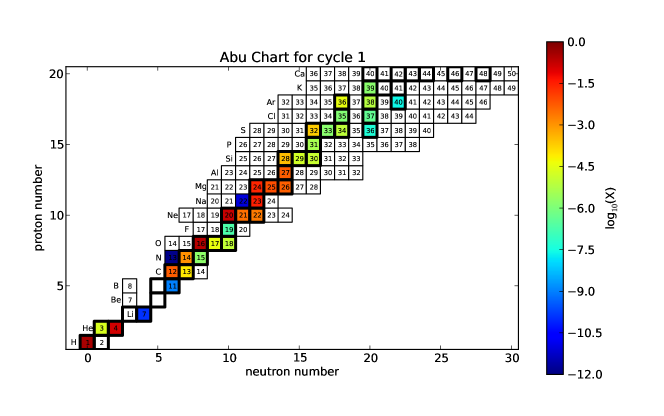
Figure 2: The isotopes and their initial abundances in the H-rich envelope of our $1.3\,M_{\odot}$ ONe nova model used in our post-processing nucleosynthesis computations.

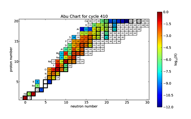
Figure 3: The isotope abundance distribution in the model in which the maximum internal temperature has reached its peak value (the red star symbol in Fig. 1). Note the accumulation of the $\beta^{+}$-unstable isotopes ¹⁴O, ¹⁵O, and ¹⁷F, also seen in the middle right panel in Fig. 1, which is typical for H-burning in the hot CNO cycle in novae.

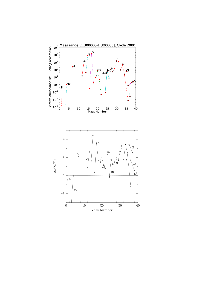
Figure 4: Upper panel: the mass-averaged abundances of stable isotopes (connected by solid and dashed lines for each element for their better identification) divided by their corresponding solar values in the expanding envelope of our final ONe nova model calculated with the NuGrid MPPNP code. Lower panel: the abundance ratios from a similar nova model (a $1.35\,M_{\odot}$ ONe WD accreting 50% pre-enriched material with the accretion rate $2\times 10^{-10}\,M_{\odot}/\mbox{yr}$) reported by the Barcelona group in [1].

The NuGrid tools have a library of Python scripts that can be used to plot MPPNP and PPN results. We have used them to produce Figs. 2, 3, 4, and 6. Fig. 2 shows the isotopes and their initial abundances that we have used in our MPPNP computations. Fig. 3 corresponds to the evolved model with $T_{\rm max}\approx 355$ MK (the red star symbol in the left panel in Fig. 1). Note the accumulation of the $\beta^{+}$-unstable isotopes ¹⁴O, ¹⁵O, and ¹⁷F, also seen in the middle right panel in Fig. 1, which is typical for H-burning in the hot CNO cycle in novae. The upper panel in Fig. 4 displays the mass-averaged abundances of stable isotopes divided by their corresponding solar values in the expanding envelope of our final model. They are compared with the abundance ratios from a similar nova model (a $1.35\,M_{\odot}$ ONe WD accreting 50% pre-enriched material with $\dot{M}=2\times 10^{-10}\,M_{\odot}/$yr) reported by the Barcelona group in [1]. In spite of the different input physics and computer codes, there is a very good qualitative agreement between the two plots.

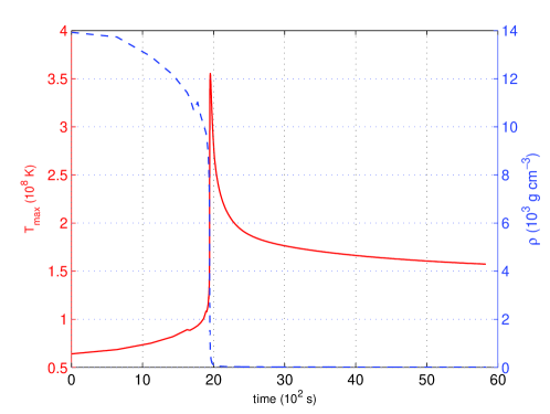
Figure 5: The trajectory ($T$ and $\rho$ as functions of time) for the Lagrangian coordinate at which the temperature profile has its maximum (e.g., see the red curve in the upper right panel in Fig. 1), extracted from our ONe nova simulations (from the file work/LOGS/star.log).

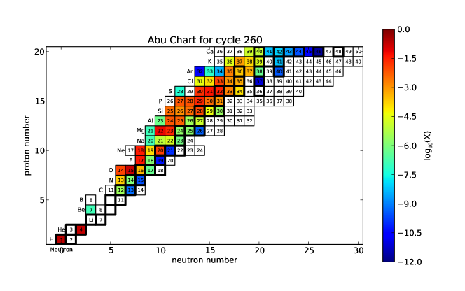
Figure 6: The distribution of isotope abundances at the time when $T$ reaches its maximum on the trajectory from Fig. 5, obtained with the NuGrid PPN code. Compare this distribution with the one from Fig. 3.

Finally, Fig. 5 shows the trajectory ($T$ and $\rho$ as functions of time) for a Lagrangian coordinate at which the temperature profile has its maximum. It can be used by the NuGrid PPN code to carry out the one-zone post-processing nucleosyntheis computations. The PPN code runs much faster than MPPNP, while producing qualitatively similar results (compare Figs. 3 and 6), therefore it can be used for a comprehensive numerical analysis of parameter space, when the isotope abundances and reaction rates are varied within their observationally and experimentally constrained limits.

- [1] J. José, & M. Hernanz, M., 1998, ApJ 494, 680
- [2] B. Paxton, L. Bildsten, A. Dotter, F. Herwig, P. Lessafre, & F. Timmes, 2011, ApJS 192, 3