A simpler load-balancing algorithm for range-partitioned data in Peer-to-Peer systems

Abstract

Random hashing is a standard method to balance loads among nodes in Peer-to-Peer networks. However, hashing destroys locality properties of object keys, the critical properties to many applications, more specifically, those that require range searching. To preserve a key order while keeping loads balanced, Ganesan, Bawa and Garcia-Molina proposed a load-balancing algorithm that supports both object insertion and deletion that guarantees a ratio of 4.237 between the maximum and minimum loads among nodes in the network using constant amortized costs. However, their algorithm is not straightforward to implement in real networks because it is recursive. Their algorithm mostly uses local operations with global max-min load information. In this work, we present a simple non-recursive algorithm using essentially the same primitive operations as in Ganesan et al.’s work. We prove that for insertion and deletion, our algorithm guarantees a constant max-min load ratio of 7.464 with constant amortized costs.

1 Introduction

One of important issues in Peer-to-Peer (P2P) networks is load balancing. Load balancing is a method that balances loads among nodes in the networks. In P2P networks, a standard technique usually used to spread keys over nodes is hashing. The research on the construction of distributed hash tables (DHTs) is very active recently. However, hashing destroys locality properties of keys. This makes many applications difficult to support a range searching.

Ganesan, Bawa and Garcia-Molina [4] proposed a sophisticated load-balancing algorithm on top of linearly ordered buckets. Since the ordering of keys is preserved, item searching is simple and range searching is naturally supported. Their algorithm, called the AdjustLoad algorithm, uses two basic balancing operations, NbrAdjust and Reorder with global max-min information, and can maintain a good ratio of 4.237 between the maximum and minimum loads among nodes in the network, while requiring a constant amortized work per operation. We give the description of their algorithm in Section 3.3.

Although both operations are easy to state, the AdjustLoad algorithm is recursive; thus, it is not straightforward to implement in distributed environments. Also, in the worst case, the AdjustLoad algorithm does not guarantee the number of invoked balancing operations, the number of updated data (partition change and load information) and the number of affected nodes. Since each balancing operation may require global information, the number of global queries may be higher than the number of insertions and deletions.

In this paper, we present a simpler, non-recursive load-balancing algorithm that uses the same primitive operations, NbrAdjust and Reorder as in Ganesan et al., but for each insertion or deletion, primitive operations are called at most once. This also implies that our proposed algorithm only makes queries to global at most once per insertion or deletion.

As in Ganesan et al., we prove that the ratio between the maximum load and the minimum load, the imbalance ratio, is at most 7.464 and the amortized cost of the algorithm is a constant per operation.

Our algorithm uses two high-level operations, MinBalance and Split:

1. The MinBalance operation occurs when there is an insertion at some node $u$ causing the load of $u$ to be too high; in this case, we shall take the node $v$ with the minimum load, transfer its load to one of $v$’s neighbors with a lighter load, and let $v$ share half the load with $u$.

2. The Split operation occurs when there is a deletion at some node $u$ causing the load of $u$ to be too low; in this case, we either let $u$ take some load from one of its neighbors, or transfer all $u$’s load to its neighbors and let it share half the load with the maximum loaded node.

Overview of the techniques. When considering only insertion, the key to proving the imbalance ratio is to analyze how the load of neighbors of the minimum loaded node changes over time. Let $z$ denote the lightly-loaded neighbor of $v$. The bad situation can occur when $z$ takes entire loads of the minimum loaded nodes (at various points in time) for too many times; this could cause the load of $z$ to be too high compared with the minimum load. We show that this is not possible because each time a load is transferred to $z$, the minimum load is increased to within some constant factor of the load of $z$, thus keeping the imbalance ratio bounded.

We make an important assumption in our analysis of the insertion-only case, namely, that the minimum load can never decrease. For the general case, this is not true. We maintain the general analysis framework by introducing the notion of phases such that within a phase the minimum load remains monotonically non-decreasing. To prove the result in this case, we show that inside a phase, the imbalance ratio is small; and when we enter a new phase (i.e., when the minimum load decreases), we are in a good starting condition.

Organization. The remainder of the paper is organized as follows. In Section 2, we discuss related work. Section 3 describes the model, states the basic definitions and reviews the AdjustLoad algorithm. In Section 4, we consider the insert-only case. We propose the MinBalance operation, analyze the imbalance ratio and calculate the cost of the algorithm. In Section 5, we consider the general case, which has both insertion and deletion. We propose the Split operation that is used when a deletion occurs and analyze the imbalance ratio and the cost of the load-balancing algorithm.

2 Related work

Research on complex queries in P2P networks has long been an interesting problem. It started when Harren et al. [5] argued that complex queries are important open issues in P2P networks. After that, much research has appeared on search methods in P2P networks. For more information, readers are referred to the survey on searching in P2P networks by Risson and Moors [15].

Range searching is one of the search methods that arises in many fields including P2P systems. Since most data structures for distributed items are based on distributed hash tables (DHTs) [11, 14, 16, 17, 20], early work focused mainly on building range search data structures on top of DHTs, e.g., PHT [13] and DST [21], based on binary search trees and segment trees, respectively. These data structures do not address a load-balancing mechanism when supporting insertion and deletion. Moreover, hot spots may occur when loads are highly imbalanced.

There are other data structures for range searching in P2P networks, which are not based on DHTs. SkipNet [6], which is adapted from Skip Lists [12], can support range searching or load balancing but not both. Skip Graphs [1] is also adapted from Skip Lists and addresses on the range searching but it does not address on load balancing on the number of items per nodes.

Many data structures support efficient range queries and show a good load balancing property in experiments, e.g., Mercury [2], Baton [7], Chordal graph [8], Dak [18] and Yarqs [19]. However, they do not have any theoretical guarantees on load distribution among nodes in their data structures.

There are mainly two groups of researchers trying to address both range searching and load-balancing theoretically. The former is the group of Karger and Ruhl [9, 10]. The latter is the group of Ganesan and Bawa [3] and Ganesan, Bawa and Garcia-Molina [4]. Both of them use two operations. The first operation balances loads between two consecutive nodes by transferring the load from the node with higher load to the node with lower load. For the second operation, a node $i$ transfers its entire load to its neighbor and relocates its position to share load with a node $j$ in a new position.

Karger and Ruhl [9, 10] presented the randomized protocol, where each node chooses another node to perform a balancing operation at random. Load balancing operations should be performed regularly, even when there is no insertion or deletion at the node. More precisely, they showed that if each node contacts $\Omega(\log n)$ other nodes then the load of each node is between $\frac{\epsilon}{16}\cdot L$ and $\frac{16}{\epsilon}\cdot L$, where $L$ denotes the average load and $\epsilon$ is a constant with $0<\epsilon<\frac{1}{4}$, with high probability, where the hidden constant in the $\Omega$ notation depends on $\epsilon$. They also showed that the cost of load balancing steps can be amortized over the constant costs of insertion and deletion. Again, the constants depend on the value of $\epsilon$. We note that this implies a high probability bound of at least 4,096 for the imbalance ratio.

Ganesan and Bawa [3] and Ganesan, Bawa and Garcia-Molina [4] proposed a distributed load-balancing algorithm that works on top of any linear data structures of items. Their algorithm is recursive and uses information about the maximum and minimum-loaded nodes. They guarantee a constant imbalance ratio with a constant cost per insertion and deletion. The ratio can be adjusted to $4.237$. This is much smaller than that of Karger and Ruhl. The major drawback is that their algorithm requires global knowledge of the maximum and minimum-loaded nodes. While this issue is important in practice (e.g., when building real P2P systems), the cost of finding global information can be amortized over the cost of other operations, e.g., node searching. For completeness, we discuss how to obtain this global information in Section 6.

3 Problem setup, cost model and the algorithm of Ganesan et al.

In this section, we describe the problem setup, discuss the cost of an algorithm and review the algorithm of Ganesan et al., the AdjustLoad algorithm.

3.1 Problem setup

We follow closely the basic setup of [4]. The system consists of $n$ nodes and maintains a collection of keys. Let $V$ be the set of all nodes. The key space is partitioned into $n$ ranges, with boundaries $R_{0}\leq R_{1}\leq\cdots\leq R_{n}$. Let $N_{i}$ be the $i$-th node that manages a range $[R_{i-1},R_{i})$. For any node $u\in V$, let $L(u)$ be the number of keys stored in $u$. At any point of time, there is an ordering of the nodes. This ordering defines left and right relations among nodes and this relation is crucial to our analysis.

As in previous work, in some operation, a node requires non-local information, namely the maximum and minimum loads and the locations of the nodes with the maximum and minimum loads.

When a key is inserted or deleted, the node that manages the range containing the key must update its data. After that, the load-balancing algorithm is invoked. Our goal is to maintain the ratio of the maximum load to the minimum load, called the imbalance ratio. We say that a load-balancing algorithm guarantees an imbalance ratio $\sigma$ if after each insertion or deletion of a key and the execution of the algorithm, $\max_{u}L(u)\leq\sigma\cdot\min_{u}L(u)+c_{0}$ for some constant $c_{0}$.

We assume that, initially, each node has a small constant load, $c_{0}$. As in [4], we ignore the concurrency issues and consider only the serial schedule of operations.

3.2 The cost

To analyze the cost of a load-balancing algorithm, we follow the three types of costs discussed in Ganesan et al..

1. Data Movement. Each operation that moves a key from one node to another is counted as a unit cost.

2. Partition Change. When load-balancing steps are performed, the range of keys stored in each node may change. This change has to be propagated through the system so that the next insertion or deletion goes to the right node.

3. Load Information. This work occurs when a node requests non-local information, e.g., requesting the node with the minimum or maximum load.

In this paper, we analyze the amortized cost of the load-balancing algorithm, i.e., we consider the worst-case cost of a sequence of $m$ load-balancing steps instead of a single one.

As in Ganesan et al., we first analyze a simpler model that accounts only for the data movement cost. For partition change cost and load information cost, we assume that there is a centralized server which maintains the partition boundaries of each node and can answer the request for global information.

This assumption can be removed as shown in Ganesan et al.. For completeness, we discuss this in Section 6.

3.3 The algorithm of Ganesan et al.

We briefly review the algorithm introduced in [4], the AdjustLoad algorithm. The algorithm uses two basic operations, NbrAdjust and Reorder operations, defined as follows.

NbrAdjust: Node $N_{i}$ transfers its load to its neighbor $N_{i+1}$. This may change the boundary $R_{i}$ of $N_{i}$ and $N_{i+1}$.

Reorder: Consider a node $N_{i}$ with an empty range $\left[R_{i},R_{i}\right)$. $N_{i}$ relocates its position and separates the range of $N_{j}$. Then, the range $\left[R_{j},X\right)$ is managed by $N_{j}$, whereas the range $\left[X,R_{j+1}\right)$ is managed by $N_{i}$ for some $X,R_{j}\leq X\leq R_{j+1}$. Finally, rename nodes appropriately.

For some constant $c$ and $\delta$, they define a sequence of thresholds $T_{m}=\left\lfloor c\delta^{m}\right\rfloor$, for all $m\geq 1$, used to trigger the AdjustLoad procedure described later. When $\delta=2$, they call their algorithm the Doubling Algorithm. The AdjustLoad procedure works as well when $\delta>\phi=\frac{(1+\sqrt{5})}{2}\approx 1.618$, the golden ratio. They call their algorithm that operates at that ratio, the Fibbing Algorithm. They prove that the AdjustLoad procedure running on that ratio would guarantee the imbalance ratio $\sigma$ of $\delta^{3}\approx 4.237$.

Given the threshold sequence, the AdjustLoad procedure is as follows. When a node $N_{i}$’s load crosses a threshold $T_{m}$, the load-balancing algorithm is invoked on that node. Let $N_{j}$ be the lightly-loaded neighbor of $N_{i}$. If the load of $N_{j}$ is not too high, the NbrAdjust operation is applied, following by two recursive calls of AdjustLoad on $N_{i}$ and $N_{j}$. Otherwise, it checks the load of the minimum-loaded node $N_{k}$, and if the imbalance ratio is too high, tries to balance the loads with the Reorder operation as follows. First, $N_{k}$ transfers its load to its lightly-loaded neighbor $N$. Then, the Reorder operation is invoked on $N_{k}$ and $N_{i}$, and finally another call to the AdjustLoad procedure is invoked on node $N$.

4 The algorithm for the insert-only case

In this section, we present the algorithm for the insert-only case. This case is simpler to analyze and provides general ideas on how to deal with the general case. It is also of practical interest because in many applications, as in a file sharing, deletions rarely occur.

We present the MinBalance procedure which uses the same primitive operations, the NbrAdjust and Reorder operations. However, it is simpler than the algorithm AdjustLoad of Ganesan et al. Notably, the MinBalance procedure is not recursive and performs only a constant number of primitive operations. We prove the bound on the imbalance ratio of 7.464 and show that the amortized cost of an insertion is a constant.

4.1 The MinBalance operation

After an insertion occurs on any node $u$, the MinBalance operation is invoked. If the load of $u$ is more than $\alpha$ times the load of the current minimum-loaded node $v$, node $v$ transfers its entire load to one of its neighbor nodes, which has a lighter load. After that, $v$ halves the load of $u$. We call these steps, MinBalance steps. Note that this procedure requires information about the minimum load; the system must maintain this information.

Procedure MinBalance $(u)$

1:  Let $v$ be the minimum-loaded node in the system.

2:  if $L(u)>\alpha\cdot L(v)$ then

3:     //MinBalance steps

4:     Let $z$ be the lightly-loaded neighbor of $v$.

5:     Transfer all keys of $v$ to $z$.

6:     Transfer a half-load of $u$ to $v$, s.t., $L(u)=\left\lceil\frac{L(u)}{2}\right\rceil$ and $L(v)=\left\lfloor\frac{L(u)}{2}\right\rfloor$.

7:     {Rename nodes appropriately.}

8:  end if

4.2 Analysis of the imbalance ratio for the insert-only case

We assume the notion of time of the system in a natural way. For simplicity, we assume that each operation completes instantly.

For any time $t$, let $L_{t}(u)$ and $L^{\prime}_{t}(u)$ denote the load of node $u$ after time $t$ and right before time $t$, i.e., $t-\epsilon$ for some $\epsilon>0$, respectively. Let $Min_{t}$ and $Min^{\prime}_{t}$ denote the minimum load in the system after time $t$ and right before time $t$ respectively, i.e., $Min_{t}=\min_{u\in V}L_{t}(u)$ and $Min^{\prime}_{t}=\min_{u\in V}L^{\prime}_{t}(u)$.

We shall prove that the following invariant holds all the time.

For any time $t$, the load of any node is not over $(\alpha+2)$ times the minimum load.

Note that the ratio of the maximum load to the minimum load is bounded by $\alpha+2$, i.e., $\frac{Max_{t}}{Min_{t}}\leq(\alpha+2)$ where $Max_{t}$ is the maximum load at time $t$. We prove this invariant in Theorem 1.

4.2.1 Overview of the analysis

While the analysis is rather involved, the idea is not very difficult to understand. This section gives an short overview to the analysis.

The main idea of the analysis is to prove that the imbalance ratio remains under a constant after any operation. We assume that the system starts with a uniform load distribution. We first show the key property for the insert-only case, that is, the minimum load never decreases. Then, we analyze how the insertions change the loads of the nodes.

When an insertion occurs on any node $u$, there are two cases depending on if $u$ calls MinBalance steps or not. After insertion, the bound on the load of $u$ itself can be verified easily.

However, the insertion also affects two other nodes, i.e., the minimum loaded node $v$ and its lighter neighbor $z$. When MinBalance steps are invoked, the minimum loaded node $v$ transfers its entire load to $z$ and shares a half load of $u$. While showing the bound on the load of $v$ is pretty straight-forward, the bound on $z$ requires more analysis because $z$ may receive loads many times through out the execution of the algorithm. The harder case for showing the bound on $z$ is when $z$ repeatedly takes loads from its neighbors without any insertions to $z$. However, in that case, we know that $z$’s neighbors at some point become the minimum loaded node; thus, we can establish the bound on the load of $z$ relative to the minimum load and prove the required ratio.

4.2.2 The analysis of the imbalance ratio

First, we show an important property of the minimum load in the system, i.e., after any operation, the minimum load never decreases.

Lemma 1

Suppose $\alpha>2$. Then the minimum load of the system never decreases.

Proof: Inserting keys into the system only increases load. The only steps that decrease loads are the MinBalance steps; therefore, we consider only these steps. For each MinBalance steps, there are three nodes involved, i.e., node $u$ which initiates the MinBalance steps at some time $t$, the current minimum-loaded node $v$ and node $z$ which is the lightly-loaded neighbor of $v$ at time $t$. First, $v$ transfers its entire keys to $z$; hence $z$’s load increases. The new load of each of $u$ and $v$ is a half of $u$’s current load. Since $u$ invokes the MinBalance steps, its load must more than $\alpha\cdot Min_{t}>2\cdot Min_{t}$. Thus, we have that after the steps, $u$’s load and $v$’s load are at least $Min_{t}$ as required.  

After an insertion occurs on any node $u$, the load of $u$ changes. Next lemma guarantees a good ratio on node $u$.

Lemma 2

Consider an insertion occurring on node $u$ at some time $t$. Suppose $\alpha\geq 3$. After an insertion and its corresponding load-balancing steps, $L_{t}(u)\leq\alpha\cdot Min_{t}$.

Proof: After an insertion, we consider two cases. The first case is when the MinBalance steps are invoked. After that the load of $u$ decreases by half. Note that the load of $u$ after insertion cannot be over $(\alpha+2)\cdot Min^{\prime}_{t}+1$ which comes from the invariant and a key insertion. Then, we have that

$$L_{t}(u)\leq\left\lceil\frac{(\alpha+2)\cdot Min^{\prime}_{t}+1}{2}\right\rceil\leq\frac{(\alpha+2)\cdot Min^{\prime}_{t}+Min^{\prime}_{t}}{2}.$$

For any $\alpha\geq 3$, it follows that $\frac{(\alpha+3)}{2}\leq\alpha$. Hence, $L_{t}(u)\leq\alpha\cdot Min^{\prime}_{t}$. From the non-decreasing property, we have $L_{t}(u)\leq\alpha\cdot Min_{t}$.

We are left to consider the second case when the MinBalance steps are not invoked. From the algorithm, the load of $u$ in this case is not over $\alpha\cdot Min^{\prime}_{t}$. Because the minimum load never decreases, we have $L_{t}(u)\leq\alpha\cdot Min_{t}$.  

Note that the MinBalance procedure “sees” the load of the newly inserted node and the minimum load, while it ignores the load of node $z$, the previous neighbor of the minimum-loaded node. We define the min-transfer event, i.e., we say that a min-transfer event occurs on node $z$, when the minimum-loaded node transfers its load to $z$, its lightly-loaded neighbor. Most of our analysis deals with the load of nodes suffered from this kind of transfer.

Consider a sequence of min-transfer events occurring on node $z$. Let $t_{i}$ represent the time after the $i$-th min-transfer event occurs on $z$. Note that before a min-transfer event occurs on $z$, an insertion may occur on it. Next lemma shows that the load of $z$ has a good ratio in this case.

Lemma 3

Suppose that an insertion occurs on node $z$ at some time $t$ right before the $i$-th min-transfer event occurs on $z$. Then $L_{t_{i}}(z)\leq(\alpha+1)\cdot Min_{t_{i}}$.

Proof: From Lemma 2, after an insertion occurs on $z$ at some time $t$, $L_{t}(z)\leq\alpha\cdot Min_{t}$. The load of $z$ increases again when the $i$-th min-transfer event occurs at time $t_{i}$. Thus,

$$L_{t_{i}}(z)=L_{t}(z)+Min^{\prime}_{t_{i}}\leq\alpha\cdot Min_{t}+Min^{\prime}_{t_{i}}.$$

Therefore, we have that $L_{t_{i}}(z)\leq(\alpha+1)\cdot Min_{t_{i}}$ because of the non-decreasing property of the minimum load.  

As the result of Lemma 3, later when dealing with the load of node $z$, we only have to consider the case that no insertion occurs on $z$ before a min-transfer event occurs on it.

In our analysis, we categorize a min-transfer event into two types: the left-transfer event and the right-transfer event. The left-transfer event on $z$ is a min-transfer event that $z$ gets the keys from the node, which is to the left of $z$ (see Figure 1 (a)). The right-transfer event on $z$ is a min-transfer event that $z$ gets the keys from the node, which is to the right of $z$ (see Figure 1 (b)).

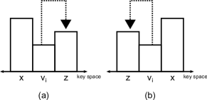
Figure 1: (a) The left-transfer event on z. (b) The right-transfer event on z.

When a new min-transfer event occurs on $z$, there are two situations, i.e., the new min-transfer event is the same type as the previous min-transfer event and the new min-transfer event is the other type.

The next lemma bounds the load of $z$ when $l$ min-transfer events of the same type occur on $z$ (probably not one after another). Note that, it is straightforward to show that the bound of $(\alpha+l+2)$ but we need a better bound.

Lemma 4

Suppose $\alpha\geq 1+\sqrt{5}\approx 3.237$ and $l\geq 0$. Consider the $i$-th, $(i+1)$-th, …, $(i+l+1)$-th min-transfer events on $z$. If the $i$-th and $(i+l+1)$-th min-transfer events are of the same type, while the $(i+1)$-th, $(i+2)$-th, …, $(i+l)$-th min-transfer events are of type different from that of the $i$-th and $(i+l+1)$-th events, then after the $(i+l+1)$-th min-transfer event, $L_{t_{i+l+1}}(z)\leq(\alpha+l+1)\cdot Min_{t_{i+l+1}}$.

Proof: Without loss of generality, we assume that the $i$-th and $(i+l+1)$-th min-transfer events occurring on $z$ are the right-transfer event; and the $(i+1)$-th, $(i+2)$-th, …, $(i+l)$-th are the left-transfer event. Let $v_{i}$ be the minimum-loaded node at time $t_{i}$.

We first deal with the case that there exists an insertion occurring on $z$ between the $i$-th and $(i+l+1)$-th min-transfer events. Assume that the latest insertion occurs on $z$ right before the $k$-th min-transfer event where $i<k\leq i+l+1$. From Lemma 3, after the $k$-th min-transfer event, the load of $z$ is not over $\alpha+1$ times the minimum load at time $t_{k}$, i.e.,

$$L_{t_{k}}(z)\leq(\alpha+1)\cdot Min_{t_{k}}.$$

Since no insertion occurs on $z$ after the $k$-th min-transfer event, we have

$$L_{t_{i+l+1}}(z)\leq(\alpha+1)\cdot Min_{t_{k}}+Min_{t_{k+1}}+\cdots+Min_{t_{i+l+1}}.$$

Because the minimum load never decreases, it follows that

$$L_{t_{i+l+1}}(z)\leq(\alpha+1)\cdot Min_{t_{i+l+1}}+(i+l-k)\cdot Min_{t_{i+l+1}},$$

and finally we have $L_{t_{i+l+1}}(z)\leq(\alpha+l+1)\cdot Min_{i+l+1}$, because $k>i$.

We are left to consider the case that there is no insertion into $z$ between the $i$-th and $(i+l+1)$-th min-transfer events. We make the first claim.

Claim 1

$$L_{t_{i+l+1}}(z)\leq L_{t_{i}}(z)+(l+1)\cdot Min^{\prime}_{t_{i+l+1}}.$$

Proof: To prove the claim, we note that for any $i<j\leq i+l+1$, the load of $z$ right before the $j$-th min-transfer event is equal to its load after the $(j-1)$-th min-transfer event, i.e.,

$$L^{\prime}_{t_{j}}(z)=L_{t_{j-1}}(z).$$ (1)

Also, for any $i<j\leq i+l+1$, the load of $z$ after the $j$-th min-transfer event increases by the minimum load before time $t_{j}$, $Min^{\prime}_{t_{j}}$. Thus,

$$L_{t_{j}}(z)=L^{\prime}_{t_{j}}(z)+Min^{\prime}_{t_{j}},$$ (2)

and from Eq. (1),

$$L_{t_{j}}(z)=L_{t_{j-1}}(z)+Min^{\prime}_{t_{j}}.$$ (3)

Telescoping, we have

$$L_{t_{i+l+1}}(z)\leq L_{t_{i}}(z)+Min^{\prime}_{t_{i+1}}+Min^{\prime}_{t_{i+2}}+\cdots+Min^{\prime}_{t_{i+l+1}}\leq L_{t_{i}}(z)+(l+1)\cdot Min^{\prime}_{t_{i+l+1}}.$$

The last step is from the non-decreasing property of the minimum load; and the claim follows.  

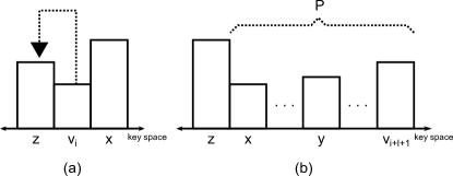
Figure 2: (a) The $i$-th min-transfer event on z. (b) The node set $P$ between $x$ and $v_{i+l+1}$.

Now, consider the $i$-th min-transfer event on $z$. Recall that the $i$-th min-transfer event is a right-transfer event. Let $x$ be the node on the right of $v_{i}$ right before the $i$-th min-transfer event occurs on $z$ (see Figure 2 (a)). Note that because the $(i+l+1)$-th min-transfer event is a right-transfer event, $x$ must become the minimum-loaded node at some point after $t_{i}$. Let $t^{*}$ be the time that $x$ becomes the minimum-loaded node after $t_{i}$. Node $x$ plays a crucial role in our analysis.

There are two cases depending on $x$ calls MinBalance steps or not.

Case 1: $x$ does not call MinBalance steps between time $t_{i}$ and $t_{i+l+1}$.

In the $i$-th min-transfer event occurring on $z$, $v_{i}$ transfers its entire load to $z$ at time $t_{i}$, but not $x$. That means the load of $z$ right before the $i$-th min-transfer event is not over the load of $x$, i.e., $L^{\prime}_{t_{i}}(z)\leq L^{\prime}_{t_{i}}(x)$. Then, after time $t_{i}$,

$$L_{t_{i}}(z)=L^{\prime}_{t_{i}}(z)+Min^{\prime}_{t_{i}}\leq L^{\prime}_{t_{i}}(x)+Min^{\prime}_{t_{i}},$$ (4)

and from the Claim 1,

$$L_{t_{i+l+1}}(z)\leq L^{\prime}_{t_{i}}(x)+Min^{\prime}_{t_{i}}+(l+1)\cdot Min^{\prime}_{t_{i+l+1}}.$$ (5)

After time $t_{i}$, $x$ becomes the minimum-loaded node at time $t^{*}$. Note that $x$ does not call the MinBalance steps. Then, the event that may occur on $x$ after time $t_{i}$ is an insertion or a min-transfer event. Thus, $x$’s load does not decrease. We have $L^{\prime}_{t_{i}}(x)\leq Min_{t^{*}}$. Then,

$$L_{t_{i+l+1}}(z)\leq Min_{t^{*}}+Min^{\prime}_{t_{i}}+(l+1)\cdot Min^{\prime}_{t_{i+l+1}}.$$

From the non-decreasing property of the minimum load, we have $L_{t_{i+l+1}}(z)\leq(l+3)\cdot Min_{t_{i+l+1}}$ and when $\alpha\geq 2$, it follows that $L_{t_{i+l+1}}(z)\leq(\alpha+l+1)\cdot Min_{t_{i+l+1}}$.

Case 2: $x$ calls MinBalance steps between time $t_{i}$ and $t_{i+l+1}$.

Let $t^{\prime}$ be the latest time that $x$ calls MinBalance steps. Since MinBalance steps are invoked, some insertion must occur on $x$. After that, $x$’s load is over $\alpha$ times the minimum load at time $t^{\prime}$. Then, the load of $x$ is divided into halves, i.e.,

$$L_{t^{\prime}}(x)\geq\left\lceil\frac{\alpha Min_{t^{\prime}}}{2}\right\rceil.$$

Note that after time $t^{\prime}$, $x$ does not call MinBalance steps and it becomes the minimum-loaded node at time $t^{*}$. The event that may occur on $x$ after time $t^{\prime}$ is an insertion or a min-transfer event. Thus, $x$’s load after time $t^{\prime}$ does not decrease. Therefore, $L_{t^{\prime}}(x)\leq L_{t^{*}}(x)$. Moreover, we know that $L_{t^{*}}(x)\leq Min^{\prime}_{t_{i+l+1}}$ by the non-decreasing property of the minimum load. Then,

$$Min^{\prime}_{t_{i+l+1}}\geq\left\lceil\frac{\alpha Min_{t^{\prime}}}{2}\right\rceil.$$ (6)

From the invariant, the load of $z$ at time $t_{i}$ is not over $(\alpha+2)$ times the minimum load at time $t_{i}$. We know that the minimum load cannot decrease; we have

$$L_{t_{i}}(z)\leq(\alpha+2)\cdot Min_{t_{i}}\leq(\alpha+2)\cdot Min_{t^{\prime}}.$$ (7)

Consider the Claim 1. We divide it by $Min_{i+l+1}$, i.e.,

$$\frac{L_{t_{i+l+1}}(z)}{Min_{i+l+1}} \leq \frac{L_{t_{i}}(z)+(l+1)\cdot Min^{\prime}_{t_{i+l+1}}}{Min_{t_{i+l+1}}}.$$

By the non-decreasing property of the minimum load, $Min^{\prime}_{t_{i+l+1}}\leq Min_{t_{i+l+1}}$. We have

$$\frac{L_{t_{i+l+1}}(z)}{Min_{i+l+1}} \leq \frac{L_{t_{i}}(z)+(l+1)\cdot Min^{\prime}_{t_{i+l+1}}}{Min^{\prime}_{t_{i+l+1}}}$$

$$= (l+1)+\frac{L_{t_{i}}(z)}{Min^{\prime}_{t_{i+l+1}}},$$

and from Eq. (6) and (7),

$$\frac{L_{t_{i+l+1}}(z)}{Min_{i+l+1}} \leq (l+1)+\frac{(\alpha+2)\cdot Min_{t^{\prime}}}{\frac{\alpha Min_{t^{\prime}}}{2}}$$

$$= (l+1)+\frac{2(\alpha+2)}{\alpha}.$$

From the assumption that $\alpha\geq 1+\sqrt{5}$, it follows that $\frac{2(\alpha+2)}{\alpha}\leq\alpha$. Then, we have

$$\frac{L_{t_{i+l+1}}(z)}{Min_{i+l+1}}\leq(\alpha+l+1).$$

 

Using previous lemmas, we can conclude the bound on the load of $z$ after a min-transfer event occurring on it.

Lemma 5

Suppose $\alpha\geq 1+\sqrt{5}\approx 3.237$. After the $i$-th min-transfer event occurs on $z$, $L_{t_{i}}(z)\leq(\alpha+2)\cdot Min_{t_{i}}.$

Proof: We prove by induction on the number of min-transfer events occurring on $z$.

For the base case, the first min-transfer event occurs on $z$. If some insertion occurs on it before the min-transfer event, t from Lemma 3, $L_{t_{1}}(z)\leq(\alpha+1)\cdot Min_{t_{1}}$. We are left to consider the case that no insertion occurs on $z$ before the first min-transfer event. The load of $z$ before the min-transfer event is equal to its load at the beginning of the system, $c_{0}$. Note that the minimum load at time $t^{\prime}_{1}$ is also $c_{0}$. After the first min-transfer event, $L_{t_{1}}(z)=2Min_{t_{1}}$. Thus, the load of $z$ in both cases is not over $(\alpha+2)\cdot Min_{t_{1}}$.

Assume that the load of any node at time $t_{k}$ is not over $(\alpha+2)\cdot Min_{t_{k}}$. Consider the $(k+1)$-th min-transfer event on $z$. There are two cases.

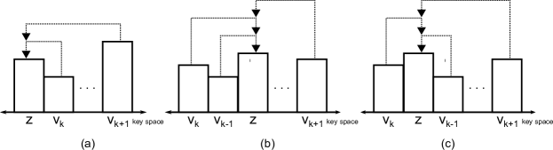
Figure 3: (a) the $k$-th and $(k+1)$-th min-transfer events are the same type. (b) the $(k-1)$-th and $k$-th min-transfer events are the same type but the $(k+1)$-th min-transfer event is a different type. (c) the $(k-1)$-th and $(k+1)$-th min-transfer events are the same type but the $k$-th min-transfer event is a different type.

Case 1: The $(k+1)$-th and $k$-th min-transfer events are the same type (see Figure 3 (a)). From Lemma 4, when set $l=0$, after the $(k+1)$-th min-transfer event, $L_{t_{k+1}}(z)\leq(\alpha+1)\cdot Min_{t_{k+1}}$. Thus, the lemma holds in this case.

Case 2: The $(k+1)$-th min-transfer event is a different type from the $k$-th min-transfer event. If there is any insertion into $z$ between time $t_{k}$ and $t_{k+1}$, from Lemma 3, $L_{t_{k+1}}(z)\leq(\alpha+1)\cdot Min_{t_{k+1}}$. We consider the $(k-1)$-th min-transfer event. There are three sub cases.

Sub case 2.1: There is no the $(k-1)$-th min-transfer event; hence, the $k$-th min-transfer event is the first min-transfer event. We can bound the load of $z$ after $t_{k}$ like the base case, i.e., $L_{t_{k}}(z)\leq(\alpha+1)\cdot Min_{t_{k}}$. The load of $z$ increases again when the $(k+1)$-th min-transfer event occurs on it at time $t_{k+1}$, i.e.,

$$L_{t_{k+1}}(z)=L_{t_{k}}(z)+Min^{\prime}_{t_{k+1}}\leq(\alpha+1)\cdot Min_{t_{k}}+Min^{\prime}_{t_{k+1}}.$$

From the non-decreasing property of the minimum load, we have that $L_{t_{k+1}}(z)\leq(\alpha+2)\cdot Min_{t_{k+1}}$. Thus, the lemma holds in this sub case.

Sub case 2.2: The $(k-1)$-th min-transfer event is the same type as the $k$-th min-transfer event (see Figure 3 (b)). From Lemma 4, when set $l=0$, after the $k$-th min-transfer event, $L_{t_{k}}(z)\leq(\alpha+1)\cdot Min_{t_{k}}$. The load of $z$ increases again by the $(k+1)$-th min-transfer event, i.e.,

$$L_{t_{k+1}}(z)=L_{t_{k}}(z)+Min^{\prime}_{t_{k+1}}\leq(\alpha+1)\cdot Min_{t_{k}}+Min^{\prime}_{t_{k+1}}.$$

From the non-decreasing property of the minimum load, we have $L_{t_{k+1}}(z)\leq(\alpha+2)\cdot Min_{t_{k+1}}$. Thus, the lemma holds in this sub case.

Sub case 2.3: The $(k-1)$-th min-transfer event is a different type from the $k$-th min-transfer event, i.e., the $(k-1)$-th min-transfer event is the same type as the $(k+1)$-th min-transfer event (see Figure 3 (c)). From Lemma 4, when set $l=1$, after the $(k+1)$-th min-transfer event, $L_{t_{k+1}}(z)\leq(\alpha+2)\cdot Min_{t_{k+1}}$ and thus, the lemma holds in this sub case.  

We are ready to prove the invariant. Note that a load of any node may change from insertion or min-transfer event. From Lemma 2 and 5, we can conclude the invariant, which guarantees the bound of any load in the system.

Theorem 1

Consider the insert-only case. Suppose $\alpha\geq 1+\sqrt{5}\approx 3.237$. For any node $u\in V$, after any event at time $t$, $L_{t}(u)\leq(\alpha+2)\cdot Min_{t}.$

In our load-balancing algorithm, we want to minimize the number of moving keys and to guarantee a constant imbalance ratio. Imbalance ratio, $\sigma$, is defined as the ratio of the maximum to minimum load in the system. We show that the imbalance ratio from our algorithm in the insert-only case is a constant.

Corollary 1

Consider the insert-only case. Suppose $\alpha\geq 1+\sqrt{5}\approx 3.237$. The imbalance ratio of the algorithm is a constant.

Proof: Prove directly from Theorem 1.  

4.3 Cost of the algorithm in insert-only case

Our algorithm uses two operations, i.e., insert and MinBalance operations. We consider the cost of each operation. Moving a single key from one node to another is counted as a unit cost. We follow the analysis in [4] based on the potential function method, and use the same potential function.

Theorem 2

Suppose that $\alpha>2(1+\sqrt{3})\approx 5.464$. The amortized costs of our algorithm in the insert-only case are constant.

Proof: Let $\bar{L}_{t}$ denote the average load at time $t$ and let $N_{i}$ be the $i$-th node that manages a range $[R_{i-1},R_{i})$. We consider the same potential function as [4], i.e., $\Phi=\frac{c\left(\sum^{n}_{i=1}(L_{t}(N_{i}))^{2}\right)}{\bar{L}_{t}}$, where $c$ is a constant to be specific later. We show that the gain in potential when an insertion occurs is at most a constant and the drop in potential when a MinBalance operation occurs pays for the cost of the operation.

Insertion: Consider an insertion of a key occurring on node $N_{j}$ at time $t$ before any load-balancing steps are invoked. Note that, the load of all nodes except $N_{j}$ does not change during the insertion. Thus, the gain in potential, $\Delta\Phi$, is

$$\Delta\Phi = \frac{c\left(\sum^{n}_{i=1}(L_{t}(N_{i}))^{2}\right)-c\left(L_{t}(N_{j})\right)^{2}+c\left(L_{t}(N_{j})+1\right)^{2}}{\bar{L}_{t}+\frac{1}{n}}-\frac{c\left(\sum^{n}_{i=1}(L_{t}(N_{i}))^{2}\right)}{\bar{L}_{t}}$$

$$\leq \frac{c\left((L_{t}(N_{j})+1)^{2}\right)-c\left(L_{t}(N_{j})^{2}\right)}{\bar{L}_{t}}$$

$$= \frac{c\left(2L_{t}(N_{j})+1\right)}{\bar{L}_{t}}.$$

From the invariant, $L_{t}(N_{j})\leq(\alpha+2)\cdot Min_{t}$. Since $\bar{L}_{t}\geq Min_{t}\geq 1$, then $L_{t}(N_{j})\leq(\alpha+2)\cdot\bar{L}_{t}$. Hence,

$$\Delta\Phi \leq \frac{c\left(2(\alpha+2)\cdot\bar{L}_{t}+1\right)}{\bar{L}_{t}}\leq c\left(2\cdot\alpha+5\right).$$

Since an insertion moves a new key to some node, the actual cost of an insertion is a unit cost. Thus, the amortized cost of an insertion is bounded by a constant.

MinBalance: There are three nodes involved, i.e., $N_{j}$ which calls MinBalance steps, the minimum-loaded node $N_{k}$ and the $N_{k}$’s lightly-loaded neighbor $N_{l}$. When node $N_{j}$ calls MinBalance steps, $N_{k}$ transfers its entire load to $N_{l}$. After that, $N_{k}$ shares a half the load of $N_{j}$. The drop potential is

$$\Delta\Phi = \frac{c\left(L_{t}(N_{j})^{2}+L_{t}(N_{k})^{2}+L_{t}(N_{l})^{2}-2(\frac{L_{t}(N_{j})}{2})^{2}-(L_{t}(N_{k})+L_{t}(N_{l}))^{2}\right)}{\bar{L}_{t}}$$

$$= \frac{c\left(\frac{L_{t}(N_{j})^{2}}{2}-2L_{t}(N_{k})L_{t}(N_{l})\right)}{\bar{L}_{t}}.$$

From the invariant, we have $L_{t}(N_{l})\leq(\alpha+2)\cdot L_{t}(N_{k})$. Since $N_{j}$ calls the MinBalance steps, we know that $L_{t}(N_{k})\leq\frac{L_{t}(N_{j})}{\alpha}$. We have $L_{t}(N_{l})\leq(\alpha+2)\cdot\frac{L_{t}(N_{j})}{\alpha}$. Then,

$$\Delta\Phi \geq \frac{c\left(\frac{L_{t}(N_{j})^{2}}{2}-\frac{2(\alpha+2)\cdot L_{t}(N_{j})^{2}}{\alpha^{2}}\right)}{\bar{L_{t}}}$$

$$= \frac{c\left(L_{t}(N_{j})^{2}(\frac{1}{2}-\frac{2(\alpha+2)}{\alpha^{2}})\right)}{\bar{L_{t}}}.$$

Again, from the invariant, we have $\bar{L_{t}}\leq(\alpha+2)\cdot L_{t}(N_{k})\leq(\alpha+2)\cdot L_{t}(N_{j})$. Then,

$$\Delta\Phi \geq cL_{t}(N_{j})\left(\frac{1}{2(\alpha+2)}-\frac{2}{\alpha^{2}}\right).$$

The data movement of MinBalance steps is $\left\lfloor\frac{L_{t}(N_{j})}{2}\right\rfloor$+ $L_{t}(N_{k})<L_{t}(N_{j})$. For any $c>\left(\frac{2\alpha^{2}(\alpha+2)}{\alpha^{2}-4(\alpha+2)}\right)$ and $\alpha>2(1+\sqrt{3})\approx 5.464$, we have $\Delta\Phi\geq L_{t}(N_{j})$. Thus, the data movement cost can be paid by this drop in potential.  

5 The algorithm for the general case

In this section, we consider the general case that supports both insert and delete operations. In order to deal with the imbalance ratio, after these operations, load balancing steps are invoked. For insertion, we perform the MinBalance operation presented in the previous section. On the other hand, for deletion, we present the Split operation.

5.1 The Split operation

The Split operation is invoked after a deletion occurs on any node $u$. Let $z$ be the lightly-loaded neighbor of $u$. The load-balancing steps are called when the load of $u$ is less than $\frac{1}{\beta}$ fractions of the maximum load at that time. There are two types of load-balancing steps depending on the load of $z$. If the load of $z$ is more than $\frac{2}{\beta}$ fractions of the maximum load, $u$ averages out its load with $z$. We call these steps, the SplitNbr. In other case, $u$ transfers its entire load to $z$. After that, $u$ shares a half load of the maximum-loaded node. These steps are called the SplitMax. Note that the SplitNbr calls only the NbrAdjust operation but the SplitMax calls both the NbrAdjust and the Reorder operations.

We again note that to be able to perform these operations, the system must maintain non-local information, i.e., the maximum load.

Procedure Split $(u)$

1:  Let $w$ be the maximum-loaded node in the system.

2:  if $L(u)\leq\frac{L(w)}{\beta}$ then

3:     Let $z$ be the lightly-loaded neighbor of $u$.

4:     if $L(z)\leq 2\cdot\frac{L(w)}{\beta}$ then

5:        //SplitMax steps

6:        Transfer all keys of $u$ to $z$.

7:        Transfer a half-load of $w$ to $u$, s.t., $L(w)=\left\lceil\frac{L(w)}{2}\right\rceil$ and $L(u)=\left\lfloor\frac{L(w)}{2}\right\rfloor$.

8:     else

9:        //SplitNbr steps

10:        Move keys from $z$ to $u$ to equalize load, s.t., $L(u)=\left\lceil\frac{(L(u)+L(z))}{2}\right\rceil$ and $L(z)=\left\lfloor\frac{(L(u)+L(z))}{2}\right\rfloor$.

11:     end if

12:     {Rename nodes appropriately.}

13:  end if

5.2 Analysis of imbalance ratio for the general case

We assume the notion of time and the invariant in the same way as the previous section. We analyze the imbalance ratio after any event. In previous section, we analyze the ratio after insertion and min-transfer event. In this section, we have to deal with deletion and two more events:

• The nbr-transfer event on node $z$ is the event that occurs when $z$ receives load from its neighbor, which invokes the SplitMax steps, and

• The nbr-share event on node $z$ is the event that occurs when $z$ shares load with its neighbor, which invokes the SplitNbr steps.

Let $Max_{t}$ and $Max^{\prime}_{t}$ denote the maximum load in the system after time $t$ and right before time $t$ respectively, i.e., $Max_{t}=\max_{u\in V}L_{t}(u)$ and $Max^{\prime}_{t}=\max_{u\in V}L^{\prime}_{t}(u)$.

5.2.1 Overview of the analysis

The major problem for applying the proofs in the insert-only case to the general case is the assumption that the minimum load cannot decrease over time. To handle this, we shall analyze the system in phases. Each phase spans the period where the minimum load is non-decreasing; this allows us to apply mostly the same techniques to the analyze the situation when the update does not change the analysis phase.

The only way an update could cause phase change is when there is a deletion in the minimum loaded node. In that case, we show that if there is a deletion on the minimum loaded node that starts the phase change, the ratio between the minimum load and the maximum load is bounded by a constant. This provides the sufficient initial condition for the analysis of the next phase.

5.2.2 Transition between phases

We shall analyze the transition between two consecutive phases occurring when the minimum load decreases.

Consider a deletion occurring on any nodes. Next lemma shows the load property of any node after deletion occurring on it.

Lemma 6

Suppose $\beta>3$. Consider the case that a deletion occurs on some node $u$ at some time $t$. After deletion and its corresponding load-balancing steps, $L_{t}(u)>\frac{Max_{t}}{\beta}$. Moreover, the minimum load can decrease in the case that load-balancing steps are not invoked.

Proof: After a deletion occurs on $u$, there are two cases. The first case is when load-balancing steps are not invoked. In this case, the load of $u$ after deletion is more than $\frac{Max^{\prime}_{t}}{\beta}$. Note that at time $t$, the only event that occurs in the system is a deletion on $u$. Then, the maximum load does not increase, i.e., $Max^{\prime}_{t}\geq Max_{t}$. We have that $L_{t}(u)>\frac{Max^{\prime}_{t}}{\beta}\geq\frac{Max_{t}}{\beta}$.

We are left to consider the second case when load-balancing steps are invoked. In this case, the load of $u$ is not over $\frac{Max^{\prime}_{t}}{\beta}$. Let $z$ be the lightly-loaded neighbor of $u$ at time $t$. There are two sub cases.

Sub case 1: Node $u$ calls SplitMax steps. First, $u$ transfers its entire load to $z$. After that, $u$ shares a half load of the maximum-loaded node, i.e.,

$$L_{t}(u)=\left\lfloor\frac{Max^{\prime}_{t}}{2}\right\rfloor>\frac{Max^{\prime}_{t}}{\beta}.$$

In this sub case, the node except $u$ that its load increases at time $t$ is $z$. Note that, $z$ receives load from $u$, i.e.,

$$L_{t}(z)=L^{\prime}_{t}(z)+L^{\prime}_{t}(u)\leq\frac{2Max^{\prime}_{t}}{\beta}+\frac{Max^{\prime}_{t}}{\beta}\leq\frac{3Max^{\prime}_{t}}{\beta}.$$

From the assumption that $\beta>3$, $L_{t}(z)<Max^{\prime}_{t}$. Since the maximum load does not increase at time $t$. Then, we have $L_{t}(u)>\frac{Max_{t}}{\beta}$.

Sub case 2: Node $u$ calls SplitNbr steps. This sub case occurs when $L^{\prime}_{t}(z)>\frac{2Max^{\prime}_{t}}{\beta}$. The load of $z$ is shared to $u$ to balance their loads, i.e.,

$$L_{t}(u)\geq\frac{\frac{2Max^{\prime}_{t}}{\beta}+L^{\prime}_{t}(u)}{2}>\frac{Max^{\prime}_{t}}{\beta}.$$

In this sub case, there are two nodes involved, $u$ and $z$. Note that the only node in the system that its load increases at time $t$ is $u$. We know that $L^{\prime}_{t}(u)\leq\frac{Max^{\prime}_{t}}{\beta}<\frac{Max^{\prime}_{t}}{2}$. Then, $u$’s load after load-balancing steps cannot over $Max^{\prime}_{t}$ because its load less than $\frac{Max^{\prime}_{t}}{2}$ and its received load cannot over $\frac{Max^{\prime}_{t}}{2}$. Since the maximum load does not increase at time $t$. Therefore, we have $L_{t}(u)>\frac{Max_{t}}{\beta}$.

Consider the load of the minimum-loaded node after deletion occurring on it at time $t$. When it is more than $\frac{Max^{\prime}_{t}}{\beta}$, load-balancing steps are not invoked. From the first case, the minimum load can decrease. When it is not over $\frac{Max^{\prime}_{t}}{\beta}$, load-balancing steps are invoked. From the second case, the load after load-balancing steps is more than $\frac{Max_{t}}{\beta}$. Thus, the minimum load does not decrease after deletion in this case.  

From Lemma 6, the minimum load at time $t$ can decrease in the case that load-balancing steps are not invoked. After the minimum load decreases at time $t$, we have $Min_{t}>\frac{Max_{t}}{\beta}$ and the phase changes. Moreover, the following condition holds:

At the beginning of each phase at time $t$, the imbalance ratio guarantee is $\beta$, i.e.,

$$\frac{Max_{t}}{Min_{t}}<\beta.$$

5.2.3 Imbalance ratio inside each phase

We prove the same invariant in the previous section, i.e.,

For any time $t$, the load of any node is not over $(\alpha+2)$ times the minimum load,

holds after each operation.

At the beginning of each phase, the imbalance load guarantee is $\beta$. At the end, we choose $\beta$ such that $\beta\leq\alpha$; this implies that at the beginning of each phase, $Max_{t}\leq\beta Min_{t}\leq(\alpha+2)Min_{t}$, as required.

In our analysis later on, we ignore the case of the deletion which is not followed with load-balancing steps, because the load of the affected can never violate the ratio. Thus, the events of this type shall not be considered in our analysis.

To analyze the imbalance ratio, we consider how the load of each affected node changes. We deal with two easy events first. For insertion, we use Lemma 2 to guarantee the load of inserted node and for deletion, we use Lemma 6 to guarantee the load of deleted node. For the rest of this section, we are left with the node which effected from load-balancing steps. There are three types of events, i.e., nbr-transfer, nbr-share and min-transfer events.

We summarize the events and how to deal with them as follows.

• For the nbr-transfer events, we focus on a lightly-loaded neighbor of the deleted node. It receives an entire load of the deleted node. Lemma 7 deals with this type of events.

• For the nbr-share events, a lightly-loaded neighbor of the deleted node averages out its load with the deleted node. The imbalance ratio is also proved in Lemma 7.

• For the min-transfer events, we focus on the load of a lightly-loaded neighbor of the minimum-loaded node. It receives load from the minimum-loaded node. Lemma 11 deals with this type of events.

The next lemma handles the case of nbr-transfer and nbr-share events.

Lemma 7

Suppose $\alpha\geq 3$ and $\beta\geq\frac{3(\alpha+2)}{\alpha}$. Consider the case that a deletion occurs on node $u$ at some time $t$ and $u$ calls load balancing steps. Let $z$ be the lightly-loaded neighbor of $u$ at time $t$. Then $L_{t}(u)\leq\alpha\cdot Min_{t}$ and $L_{t}(z)\leq\alpha\cdot Min_{t}$.

Proof: There are two types of load balancing steps after deletion.

Case 1: Node $u$ invokes SplitMax steps and a nbr-transfer event occurs on $z$. This case occurs when $L^{\prime}_{t}(z)\leq\frac{2Max^{\prime}_{t}}{\beta}$ and $L^{\prime}_{t}(u)\leq\frac{Max^{\prime}_{t}}{\beta}$. Node $u$ proceeds by transferring its entire load to $z$, i.e.,

$$L_{t}(z)\leq\frac{2Max^{\prime}_{t}}{\beta}+\frac{Max^{\prime}_{t}}{\beta}.$$

From the invariant, we have $L_{t}(z)\leq\frac{3((\alpha+2)\cdot Min^{\prime}_{t})}{\beta}$. Since $\beta\geq\frac{3(\alpha+2)}{\alpha}$, it follows that $\frac{3(\alpha+2)}{\beta}\leq\alpha$. Then, the load of $z$ at time $t$ is not over $\alpha\cdot Min^{\prime}_{t}$. From the non-decreasing property of the minimum load, we have $L_{t}(z)\leq\alpha\cdot Min_{t}$.

After that, $u$ shares half a load of the maximum-loaded node. From the invariant, we have that $L_{t}(u)\leq\frac{(\alpha+2)Min^{\prime}_{t}}{2}$. When $\alpha\geq 2$, it follows that $\frac{(\alpha+2)}{2}\leq\alpha$. Then, the load of $u$ after deletion is not over $\alpha\cdot Min_{t}^{\prime}$ and we have $L_{t}(u)\leq\alpha\cdot Min_{t}$ from the non-decreasing property of the minimum load.

Case 2: Node $u$ invokes SplitNbr steps and a nbr-share event occurs on $z$. This case occurs when $L^{\prime}_{t}(z)>\frac{2Max^{\prime}_{t}}{\beta}$ and $L^{\prime}_{t}(u)\leq\frac{Max^{\prime}_{t}}{\beta}$. From the invariant, we have $L^{\prime}_{t}(z)\leq Max^{\prime}_{t}\leq(\alpha+2)\cdot Min^{\prime}_{t}$. Node $u$ and $z$ share their loads equally, i.e.,

$$L_{t}(z)\leq\frac{(\alpha+2)\cdot Min^{\prime}_{t}+(\alpha+2)\cdot\frac{Min^{\prime}_{t}}{\beta}}{2}\leq\frac{(\beta+1)(\alpha+2)}{2\beta}\cdot Min^{\prime}_{t}.$$

From the assumption that $\alpha\geq 3$ and $\beta\geq\frac{3(\alpha+2)}{\alpha}$, we have that $\beta>\frac{(\alpha+2)}{(\alpha-2)}$. Moreover, when $\beta>\frac{(\alpha+2)}{(\alpha-2)}$ and $\alpha>2$, it follows that $\frac{(\beta+1)(\alpha+2)}{2\beta}\leq\alpha$. Then, the load of $z$ and $u$ after load-balancing steps are not over $\alpha\cdot Min^{\prime}_{t}$. From the non-decreasing property of the minimum load, we have $L_{t}(u)\leq\alpha\cdot Min_{t}$ and $L_{t}(z)\leq\alpha\cdot Min_{t}$.  

We are left with the min-transfer case. Let $e$ be the min-transfer event occurring on $z$. Next lemma deals with the case that $e$ is the first event occurring on $z$ in phase $d$.

Lemma 8

Consider any phase $d$. Suppose $\beta>2$. If the first event occurring on $z$ in that phase is the $i$-th min-transfer event, $L_{t_{i}}(z)\leq(\beta+1)\cdot Min_{t_{i}}.$

Proof: There are two cases to consider. First, we consider the case that $d=1$, i.e., the first phase. At the beginning of this phase, the load of any node is equal to $c_{0}$. Note that the load of $z$ does not change until the first min-transfer event occurs on it. Moreover, at time $t_{1}$, the minimum load is also $c_{0}$ because it cannot decrease and it cannot increase over $c_{0}$. When the min-transfer event occurs on $z$, it’s load increases, i.e., $L_{t_{1}}(z)=c_{0}+Min^{\prime}_{t_{1}}=2Min^{\prime}_{t_{1}}$. From the non-decreasing property of the minimum load, we have $L_{t_{1}}(z)\leq 2Min_{t_{1}}$. From the assumption that $\beta>2$, it follows that $L_{t_{1}}(z)\leq(\beta+1)\cdot Min_{t_{1}}$.

For the case that $d>1$, let $t^{\prime}$ be the beginning time of phase $d$. From the load condition at the beginning of each phase, $Max_{t^{\prime}}<\beta Min_{t^{\prime}}$. Therefore, $L_{t^{\prime}}(z)<\beta Min_{t^{\prime}}$. After the $i$-th min-transfer event occurs on $z$, its load increases, i.e., $L_{t_{i}}(z)=L_{t^{\prime}}(z)+Min^{\prime}_{t_{i}}\leq\beta\cdot Min_{t^{\prime}}+Min^{\prime}_{t_{i}}$. Because the minimum load never decreases in each phase, we have $L_{t_{i}}(z)\leq(\beta+1)\cdot Min_{t_{i}}$ as required.  

Now, assume that $e$ is not the first event occurring on $z$ in phase $d$.

Let $e^{\prime}$ be the latest event that occurs on $z$ before an event $e$. The next lemma considers the case where $e^{\prime}$ is not a min-transfer event, while Lemma 10, which is more involved, considers the case when $e^{\prime}$ is a min-transfer event.

Lemma 9

Consider any phase. Suppose $\alpha\geq 3$ and $\beta\geq\frac{3(\alpha+2)}{\alpha}$. If any event $e^{\prime}$ except a min-transfer event occurs on node $z$ right before the $i$-th min-transfer event, then after the $i$-th min-transfer event occurs on $z$, $L_{t_{i}}(z)\leq(\alpha+1)\cdot Min_{t_{i}}.$

Proof: An event $e^{\prime}$ can be an insertion, or a deletion which is followed with load-balancing steps, or an nbr-transfer event, or an nbr-share event. After event $e^{\prime}$ occurs on $z$ at time $t^{\prime}$, from Lemma 2 (for insertions) and Lemma 7 (for other events), we have $L_{t^{\prime}}(z)\leq\alpha\cdot Min_{t^{\prime}}$. The load of $z$ increases again from the $i$-th min-transfer event, i.e., $L_{t_{i}}(z)=L_{t^{\prime}}(z)+Min^{\prime}_{t_{i}}\leq\alpha\cdot Min_{t^{\prime}}+Min^{\prime}_{t_{i}}$. Because the minimum load does not decrease in each phase, it follows that $L_{t_{i}}(z)\leq(\alpha+1)\cdot Min_{t_{i}}$.  

Finally, we consider the case when the latest event $e^{\prime}$ before event $e$ is a min-transfer event. Recall that we categorize the min-transfer event into two types: the left-transfer event and the right-transfer event. The next lemma is a generalization of Lemma 4 but it deals more with deletion, SplitMax and SplitNbr.

Lemma 10

Suppose $\alpha\geq\frac{3+\sqrt{33}}{2}\approx 4.373$, $\beta\geq\frac{3(\alpha+2)}{\alpha}$ and $l\geq 0$. Consider the $i$-th, $(i+1)$-th, …, $(i+l+1)$-th min-transfer events on $z$ in any phase. If the $i$-th and $(i+l+1)$-th min-transfer events are of the same type, while the $(i+1)$-th, $(i+2)$-th, …, $(i+l)$-th min-transfer events are of type different from that of the $i$-th and $(i+l+1)$-th events, then after the $(i+l+1)$-th min-transfer event, $L_{t_{i+l+1}}(z)\leq(\alpha+l+1)\cdot Min_{t_{i+l+1}}$.

Proof: Without loss of generality, we assume that the $i$-th and $(i+l+1)$-th min-transfer events occurring on $z$ are right-transfer events; and the $(i+1)$-th, $(i+2)$-th, …, $(i+l)$-th are left-transfer events. Let $v_{i}$ be the minimum-loaded node at time $t_{i}$.

We first deal with the case that there exists an event except the min-transfer event occurring on $z$ between the $i$-th and $(i+l+1)$-th min-transfer events. Assume that the latest event except the min-transfer event occurs on $z$ right before the $k$-th min-transfer event where $i<k\leq i+l+1$. From Lemma 9, after the $k$-th min-transfer event, we have

$$L_{t_{k}}(z)\leq(\alpha+1)\cdot Min_{t_{k}}.$$

After the $k$-th min-transfer event, only the min-transfer event can occur on $z$. Note that after time $t_{k}$, there are at most $i+l-k$ min-transfer events occurring on $z$ at time $t_{i+l+1}$. Since, the minimum load never decreases, we have that

$$L_{t_{i+l+1}}(z)\leq(\alpha+1)\cdot Min_{t_{i+l+1}}+(i+l-k)\cdot Min_{t_{i+l+1}},$$

and finally we have $L_{t_{i+l+1}}(z)\leq(\alpha+l+1)\cdot Min_{i+l+1}$, because $k>i$.

We are left to consider the case that there is no other events occurring on $z$ except the min-transfer event between the $i$-th and $(i+l+1)$-th min-transfer events. We follow Claim 1 in the proof of Lemma 4 using the property that in each phase the minimum load does not decrease. Then, we have

$$L_{t_{i+l+1}}(z)\leq L_{t_{i}}(z)+(l+1)\cdot Min^{\prime}_{t_{i+l+1}}.$$ (8)

Consider the $i$-th min-transfer event on $z$. Recall that, it is a right-transfer event. Let $x$ be the node on the right of $v_{i}$ right before the $i$-th min-transfer event. Note that, because the $(i+l+1)$-th min-transfer event is also a right-transfer event, $x$ must become the minimum-loaded node at some point after time $t_{i}$. Let $t^{*}$ be the time that $x$ becomes the minimum-loaded node after time $t_{i}$.

Instead of focusing on node $x$, we consider a set of nodes $P$ that arranges in a consecutive order from $x$ to $v_{i+l+1}$ between time $t_{i}$ and $t_{i+l+1}$ (see Figure 2 (b)). We bound the load of $z$ by the load of node in this set. There are two cases.

Case 1: No nodes in set $P$ calls MinBalance, SplitMax and SplitNbr steps between time $t_{i}$ and $t_{i+l+1}$. In this case, we consider the node $x$. Note that deletion may occur on $x$. There are two sub cases.

Sub case 1.1: No deletion occurs on $x$ after $t_{i}$. Consider the $i$-th min-transfer event occurring on $z$. The minimum-loaded node at time $t_{i}$ transfers its load to $z$. That means $L^{\prime}_{t_{i}}(z)\leq L^{\prime}_{t_{i}}(x)$. Then, we have

$$L_{t_{i}}(z)=L^{\prime}_{t_{i}}(z)+Min^{\prime}_{t_{i}}\leq L^{\prime}_{t_{i}}(x)+Min^{\prime}_{t_{i}},$$

and from Eq. (8), we have

$$L_{t_{i+l+1}}(z)\leq L^{\prime}_{t_{i}}(x)+Min^{\prime}_{t_{i}}+(l+1)\cdot Min^{\prime}_{t_{i+l+1}}.$$ (9)

After time $t_{i}$, deletion and load-balancing steps do not occur on $x$. The operation that can occur on it is an insertion. Then, $x$’s load does not decrease. At time $t^{*}$, $x$ becomes the minimum-loaded node. Then, $L^{\prime}_{t_{i}}(x)\leq Min_{t^{*}}$. From Eq. (9), we have

$$L_{t_{i+l+1}}(z)\leq Min_{t^{*}}+Min^{\prime}_{t_{i}}+(l+1)\cdot Min^{\prime}_{t_{i+l+1}}.$$

Because the minimum load does not decrease, we have $L_{t_{i+l+1}}(z)\leq(l+3)\cdot Min_{t_{i+l+1}}$. When $\alpha\geq 2$, we have $L_{t_{i+l+1}}(z)\leq(\alpha+l+1)\cdot Min_{t_{i+l+1}}$. Thus, the lemma holds in this sub case.

Sub case 1.2: Some deletion occurs on $x$ after $t_{i}$ but SplitMax and SplitNbr steps are not invoked. Let $t^{\prime}$ be the time that $x$ has the minimum load after deletion occurring on it between time $t_{i}$ and $t^{*}$. From Lemma 6, the maximum load at time $t^{\prime}$ is not over $\beta$ times the load of $x$ at time $t^{\prime}$. Then, we have

$$Max_{t^{\prime}}\leq\beta L_{t^{\prime}}(x)\leq\beta L_{t^{*}}(x).$$ (10)

Note that the only event that can occur on $z$ between time $t_{i}$ and $t^{\prime}$ is a min-transfer event. Thus, the load of $z$ after $t_{i}$ does not decrease. Then, we have $L_{t_{i}}(z)\leq L_{t^{\prime}}(z)$. Consider Eq. (8). We have

$$L_{t_{i+l+1}}(z)\leq L_{t^{\prime}}(z)+(l+1)\cdot Min^{\prime}_{t_{i+l+1}}.$$

From Eq. (10), we have

$$L_{t_{i+l+1}}(z)\leq Max_{t^{\prime}}+(l+1)\cdot Min^{\prime}_{t_{i+l+1}}\leq\beta L_{t^{*}}(x)+(l+1)\cdot Min^{\prime}_{t_{i+l+1}}.$$

Since in each phase, the minimum load never decreases, we have $L_{t_{i+l+1}}(z)\leq(\beta+l+1)\cdot Min_{t_{i+l+1}}$. From the assumption that $\alpha\geq\frac{3+\sqrt{33}}{2}$, it follows that $\alpha\geq\beta$ and thus, the lemma holds in this sub case.

Case 2: At least one node in $P$ calls MinBalance or SplitMax or SplitNbr steps between time $t_{i}$ and $t_{i+l+1}$. Let $y$ be the latest node in this set that calls load-balancing steps at time $\hat{t}$. We consider the case that some deletion occurs on $y$ after $\hat{t}$. We can prove in the same way as sub case 1.2 and it follows that $L_{t_{i+l+1}}(z)\leq(\alpha+l+1)\cdot Min_{t_{i+l+1}}$.

We are left to consider the case that no deletion occurs on $y$ after MinBalance or SplitNbr or SplitMax steps occurring on $y$ after $\hat{t}$.

Sub case 2.1: Node $y$ calls MinBalance steps at time $\hat{t}$. This sub case can be proved in the same way as case 2 in Lemma 4. When $\alpha\geq 1+\sqrt{5}$, it follows that $\frac{L_{t_{i+l+1}}(z)}{Min_{i+l+1}}\leq(\alpha+l+1).$ Thus, the lemma holds in this sub case.

Sub case 2.2: Node $y$ calls SplitNbr steps at time $\hat{t}$. From Lemma 6, after SplitNbr steps, we have $Max_{\hat{t}}\leq\beta L_{\hat{t}}(y)$. Note that the event that occurs on $z$ after $t_{i}$ is the min-transfer event. Then, $z$’s load does not decrease after $t_{i}$. We have $L_{t_{i}}(z)\leq L_{\hat{t}}(z)$. Consider Eq. (8). Then, it follows that

$$L_{t_{i+l+1}}(z)\leq Max_{\hat{t}}+(l+1)\cdot Min^{\prime}_{t_{i+l+1}}\leq\beta\cdot L_{\hat{t}}(y)+(l+1)\cdot Min^{\prime}_{t_{i+l+1}}.$$

After time $\hat{t}$, no load-balancing steps or deletion occurs on $y$. Then, after $\hat{t}$, $y$’s load never decreases. Since the $(i+l+1)$-th min-transfer event is a right-transfer event, $y$ must become the minimum-loaded node at some point. Let $t^{{}^{\prime\prime}}$ be the time that $y$ becomes the minimum-loaded node. It follows that $L_{\hat{t}}(y)\leq L_{t^{{}^{\prime\prime}}}(y)$. Then, we have $L_{t_{i+l+1}}(z)\leq(\beta+l+1)\cdot Min_{t_{i+l+1}}$. When $\alpha\geq\frac{3+\sqrt{33}}{2}$, it follows that $\alpha\geq\beta$ and thus, the lemma holds in this sub case.

Sub case 2.3: Node $y$ calls SplitMax steps at time $\hat{t}$. After $y$ calls these steps, it transfers its entire load to its neighbor $w$. Then, we have $L_{\hat{t}}(w)\geq 2Min_{\hat{t}}$. After that, $y$ is relocated. Thus, we consider node $w$ instead.

We show that $w$ is in $P$. Assume by contradiction that $w$ is not in $P$. Note that the position of $w$ can be left or right of $y$. Consider the case that $w$ is right of $y$. $w$ can be outside $P$ when $y$ must be the rightmost node in $P$. Because $v_{i+l+1}$ is the rightmost node in $P$, this case contradicts. Consider the case that $w$ is left of $y$. In this case, $y$ must be the leftmost node in $P$ and $y$ transfers its load to the node outside $P$. Note that the node which $y$ transfers its load is $z$. This contradicts that no events occur on $z$ except the min-transfer event.

Consider the case that some deletion occurs on $w$ after $\hat{t}$. This case can be proved in the same way as sub case 1.2.

Now, we assume that no deletion occurs on $w$ after $\hat{t}$. Recall that at time $\hat{t}$, we have $2Min_{\hat{t}}\leq L_{\hat{t}}(w)$. Since the $(i+l+1)$-th min-transfer event is a right-transfer event, $w$ becomes the minimum-loaded node at some point after $\hat{t}$. Let $t^{*}$ be the time that $w$ becomes the minimum-loaded node after $\hat{t}$. After time $\hat{t}$, load-balancing steps and deletion do not occur on $w$. Then, $w$’s load does not decrease. We have $L_{\hat{t}}(w)\leq L_{t^{*}}(w)$. Moreover, we have $L_{\hat{t}}(w)\leq Min^{\prime}_{t_{i+l+1}}$ from the non-decreasing property of the minimum load. Thus, $2Min_{\hat{t}}\leq Min^{\prime}_{t_{i+l+1}}$.

Consider Eq. (8). We divide it by $Min_{i+l+1}$, i.e.,

$$\frac{L_{t_{i+l+1}}(z)}{Min_{i+l+1}} \leq \frac{L_{t_{i}}(z)+(l+1)\cdot Min^{\prime}_{t_{i+l+1}}}{Min_{i+l+1}}$$

$$\leq \frac{L_{t_{i}}(z)+(l+1)\cdot Min^{\prime}_{t_{i+l+1}}}{Min^{\prime}_{t_{i+l+1}}}$$

$$= (l+1)+\frac{L_{t_{i}}(z)}{Min^{\prime}_{t_{i+l+1}}}.$$

From the invariant, it follows that $L_{t_{i}}(z)\leq(\alpha+2)\cdot Min_{t_{i}}\leq(\alpha+2)\cdot Min_{\hat{t}}$ when $t_{i}<\hat{t}$. Recall that $2Min_{\hat{t}}\leq Min^{\prime}_{t_{i+l+1}}$. Then,

$$\frac{L_{t_{i+l+1}}(z)}{Min_{i+l+1}}\leq(l+1)+\frac{(\alpha+2)\cdot Min_{\hat{t}}}{2Min_{\hat{t}}}.$$

When $\alpha>2$, it follows that $\frac{(\alpha+2)}{2}\leq\alpha$. Then, we have $\frac{L_{t_{i+l+1}}(z)}{Min_{i+l+1}}\leq(\alpha+l+1).$ Thus, the lemma holds in this sub case.  

From Lemma 8,  9 and 10, we conclude the effect of the min-transfer event on any node $z$. We omit the proof because it is similar to the proof of Lemma 5.

Lemma 11

Consider any phase $d$. Suppose $\alpha\geq\frac{3+\sqrt{33}}{2}\approx 4.373$ and $\beta\geq\frac{3(\alpha+2)}{\alpha}$. After the $i$-th min-transfer event occurs on $z$, $L_{t_{i}}(z)\leq(\alpha+2)\cdot Min_{t_{i}}.$

Finally, we are ready to prove the imbalance ratio guarantee. In each phase, the load of any node can be changed by insertion, deletion, nbr-transfer, nbr-share and min-transfer events. From Lemma 2, 6, 7 and 11, we can conclude the upper bound of load of any node in any phase after these events.

Theorem 3

Consider any phase. Suppose $\alpha\geq\frac{3+\sqrt{33}}{2}\approx 4.373$ and $\beta\geq\frac{3(\alpha+2)}{\alpha}$. For any node $u\in V$, after any event at time $t$, $L_{t}(u)\leq(\alpha+2)\cdot Min_{t}.$ Thus, the imbalance ratio of the algorithm in the general case is a constant.

5.3 Cost of the algorithm in the general case

We analyze the cost of our algorithm in the general case. Recall that, the cost of moving a key from node $u$ to another node $v$ is counted as a unit cost. In our algorithm, there are four operations, i.e., insertion, deletion, MinBalance and Split. Again, we prove the amortized cost by potential method and use the same potential function of Ganesan et al..

Theorem 4

Suppose $\alpha>2(1+\sqrt{3})\approx 5.464$. The amortized costs of our algorithm are constant.

Proof: We use the potential function in [4], i.e., $\Phi=\frac{c(\sum^{n}_{i=1}(L_{t}(N_{i}))^{2})}{\bar{L}_{t}}$, where $\bar{L}_{t}$ is the average load at time $t$ and $N_{i}$ be the $i$-th node that manages a range $[R_{i-1},R_{i})$. We show that the gain in potential when insertion or deletion occurs is at most a constant and the drop in potential when MinBalance or Split operation occurs pays for the cost of the operation. These imply that the amortized costs of insertion and deletion are constant.

We prove the cost of insertion and MinBalance operation in the same way as Theorem 2. We are left to consider a deletion and Split operation.

Deletion: When a deletion occurs on $N_{j}$ at time $t$, the gain in potential is at most

$$\Delta\Phi \leq c\frac{\left(\sum_{i\in V}{L_{t}(N_{i})^{2}}\right)}{\left(\bar{L}_{t}-\frac{1}{n}\right)}-c\frac{\left(\sum_{i\in V}{L_{t}(N_{i})^{2}}\right)}{\bar{L}_{t}}$$

$$= c\frac{\left(\sum_{i\in V}{L_{t}(N_{i})^{2}}\right)(\frac{1}{n})}{\bar{L}_{t}\cdot\left(\bar{L}_{t}-\frac{1}{n}\right)}.$$

We know that $\bar{L}_{t}\geq Min_{t}$. From the invariant, we have that $L_{t}(u)\leq(\alpha+2)\cdot Min_{t}\leq(\alpha+2)\cdot\bar{L}_{t}$ for any node $u$. Using the fact that $\bar{L}_{t}-\frac{1}{n}\geq\frac{\bar{L}_{t}}{2}$ where $n\geq 2$ and $\bar{L}_{t}\geq 1$, we have

$$\Delta\Phi \leq c\frac{\left((\alpha+2)\cdot\bar{L}_{t}\right)^{2}}{\bar{L}_{t}\cdot\left(\frac{\bar{L}_{t}}{2}\right)}\leq 2c(\alpha+2)^{2}.$$

Hence, the amortized cost of deletion is a constant because the actual cost of deletion is a unit cost.

Split: Consider the load of node $N_{j}$, whose calls Split at time $t$. When its load is less than $\frac{Max_{t}}{\beta}$, load-balancing steps are called. There are two cases, i.e., SplitNbr and SplitMax steps.

Case SplitNbr: Let $N_{k}$ be the lightly-loaded neighbor of $N_{j}$ when $N_{j}$ calls SplitNbr steps. Node $N_{k}$ moves its keys to $N_{j}$ to balance their loads. The drop in potential is

$$\Delta\Phi = \frac{c\left(L_{t}(N_{j})^{2}+L_{t}(N_{k})^{2}-2\left(\frac{L_{t}(N_{j})+L_{t}(N_{k})}{2}\right)^{2}\right)}{\bar{L}_{t}}$$

$$= c\frac{\left(\frac{L_{t}(N_{j})^{2}}{2}+\frac{L_{t}(N_{k})^{2}}{2}-\left(L_{t}(N_{j})L_{t}(N_{k})\right)\right)}{\bar{L}_{t}}$$

$$= c\frac{\left(L_{t}(N_{k})-L_{t}(N_{j})\right)^{2}}{2\bar{L}_{t}}$$

$$= c\frac{\left(L_{t}(N_{k})-L_{t}(N_{j})\right)}{2}\frac{\left(L_{t}(N_{k})-L_{t}(N_{j})\right)}{\bar{L}_{t}}.$$

This case occurs when $L_{t}(N_{k})>\frac{2Max_{t}}{\beta}$ and $L_{t}(N_{j})<\frac{Max_{t}}{\beta}$. Then,

$$\Delta\Phi \geq c\frac{\left(L_{t}(N_{k})-L_{t}(N_{j})\right)}{2}\frac{\left(\frac{2Max_{t}}{\beta}-\frac{Max_{t}}{\beta}\right)}{\bar{L}_{t}}$$

$$= c\frac{\left(L_{t}(N_{k})-L_{t}(N_{j})\right)}{2}\frac{\left(\frac{Max_{t}}{\beta}\right)}{\bar{L}_{t}}$$

$$\geq c\frac{\left(L_{t}(N_{k})-L_{t}(N_{j})\right)}{2}\left(\frac{1}{\beta}\right).$$

The number of moved keys when SplitNbr steps are invoked is $\frac{\left(L_{t}(N_{k})-L_{t}(N_{j})\right)}{2}$. For any $c>\beta$, we have $\Delta\Phi\geq\frac{\left(L_{t}(N_{k})-L_{t}(N_{j})\right)}{2}$. Thus, the drop in potential pays for the data movement.

Case SplitMax: Node $N_{j}$ transfers its entire load to its adjacent node $N_{k}$ and then shares half the load of the maximum-loaded node $N_{l}$. The drop in potential is

$$\Delta\Phi = c\frac{\left(L_{t}(N_{j})^{2}+L_{t}(N_{k})^{2}+L_{t}(N_{l})^{2}-2\left(\frac{L_{t}(N_{l})}{2}\right)^{2}-\left(L_{t}(N_{k})+L_{t}(N_{j})\right)^{2}\right)}{\bar{L}_{t}}$$

$$= c\frac{\left(\frac{L_{t}(N_{l})^{2}}{2}-2L_{t}(N_{k})L_{t}(N_{j})\right)}{\bar{L}_{t}}$$

$$= \frac{c}{\bar{L}_{t}}L_{t}(N_{l})^{2}\left(\frac{1}{2}-\frac{2L_{t}(N_{k})L_{t}(N_{j})}{L_{t}(N_{l})^{2}}\right).$$

From the algorithm, we know that $L_{t}(N_{k})\leq\frac{2Max_{t}}{\beta}$ and $L_{t}(N_{j})\leq\frac{Max_{t}}{\beta}$. Then,

$$\Delta\Phi \geq cL_{t}(N_{l})\left(\frac{1}{2}-\frac{2\frac{2Max_{t}}{\beta}\cdot\frac{Max_{t}}{\beta}}{L_{t}(N_{l})^{2}}\right)$$

$$\geq c\cdot L_{t}(N_{l})\left(\frac{1}{2}-\frac{4}{\beta^{2}}\right).$$

When SplitMax steps are invoked, the number of moved keys is $\frac{L_{t}(N_{l})}{2}+L_{t}(N_{j})\leq L_{t}(N_{l})$. For any $c>\left(\frac{2\beta^{2}}{\beta^{2}-8}\right)$, it follows that $\Delta\Phi\geq L_{t}(N_{l})$ and thus, the drop in potential pays for the key movement.

Thus, the amortized costs of the algorithm are constant.  

6 The cost in real networks

In this section, we discuss how Ganesan et al. [4] dealt with global information and, again, discuss the comparison between this line of work, which this paper extends, and the work of Karger and Ruhl [9, 10] when considering real networks.

In the P2P networks, there is no centralized server to provide the information. If any node requires information about another node, it must send messages to that node. Besides the data movement cost, there is another cost to be considered, the communication cost. The communication cost is defined as a number of messages that required for complete the operation.

We shall discuss how Ganesan et al. implement the idea on real networks. Their implementation is based on skip graphs [1]. Skip graphs support find operation, node insertion, and node deletion with $O(\log n)$ messages with high probability. Also adjacent nodes can be contact with $O(1)$ messages. Ganesan at al. use two skip graphs: one where nodes are ordered by their minimum key in their ranges; another where nodes are ordered by their loads. Therefore, global information can be found with $O(\log n)$ messages, and each partition change costs at most $O(\log n)$ messages. We note that while this cost is more than the constant cost of data movement, usually $O(\log n)$ messages are required for finding the node for each key, and thus these cost can be amortized with the searching cost.

As in Ganesan et al. works, Karger and Ruhl [9, 10] simplify the cost model by not considering how one could find a given node in the system. Therefore, unless they maintain a global directory of nodes, using known data structures for p2p systems, they still need $O(\log n)$ messages as well.

References

- [1] J. Aspnes and G. Shah. Skip graphs. In Proceedings of the fourteenth annual ACM-SIAM symposium on Discrete algorithms, SODA ’03, pages 384–393, 2003.
- [2] A. R. Bharambe, M. Agrawal, and S. Seshan. Mercury: supporting scalable multi-attribute range queries. In Proceedings of the 2004 conference on Applications, technologies, architectures, and protocols for computer communications, SIGCOMM ’04, pages 353–366, 2004.
- [3] P. Ganesan and M. Bawa. Distributed balanced tables: Not making a hash of it all. Technical Report 2003-71, Stanford InfoLab, 2003.
- [4] P. Ganesan, M. Bawa, and H. Garcia-Molina. Online balancing of range-partitioned data with applications to peer-to-peer systems. In Proceedings of the Thirtieth international conference on Very large data bases - Volume 30, VLDB ’04, pages 444–455, 2004.
- [5] M. Harren, J. M. Hellerstein, R. Huebsch, B. T. Loo, S. Shenker, and I. Stoica. Complex queries in dht-based peer-to-peer networks. In Revised Papers from the First International Workshop on Peer-to-Peer Systems, IPTPS ’01, pages 242–259, 2002.
- [6] N. J. A. Harvey, M. B. Jones, S. Saroiu, M. Theimer, and A. Wolman. Skipnet: a scalable overlay network with practical locality properties. In Proceedings of the 4th conference on USENIX Symposium on Internet Technologies and Systems - Volume 4, USITS’03, pages 9–9, 2003.
- [7] H. V. Jagadish, B. C. Ooi, and Q. H. Vu. Baton: a balanced tree structure for peer-to-peer networks. In Proceedings of the 31st international conference on Very large data bases, VLDB ’05, pages 661–672, 2005.
- [8] Y.-J. Joung. Approaching neighbor proximity and load balance for range query in p2p networks. Comput. Netw., 52:1451–1472, May 2008.
- [9] D. R. Karger and M. Ruhl. New algorithms for load balancing in peer-to-peer systems. In IRIS Student Workshop, 2003.
- [10] D. R. Karger and M. Ruhl. Simple efficient load balancing algorithms for peer-to-peer systems. In Proceedings of the sixteenth annual ACM symposium on Parallelism in algorithms and architectures, SPAA ’04, pages 36–43, 2004.
- [11] P. Maymounkov and D. Mazières. Kademlia: A peer-to-peer information system based on the xor metric. In Revised Papers from the First International Workshop on Peer-to-Peer Systems, IPTPS ’01, pages 53–65, 2002.
- [12] W. Pugh. Skip lists: A probabilistic alternative to balanced trees, 1990.
- [13] S. Ramabhadran, S. Ratnasamy, J. M. Hellerstein, and S. Shenker. Brief announcement: prefix hash tree. In Proceedings of the twenty-third annual ACM symposium on Principles of distributed computing, PODC ’04, pages 368–368, 2004.
- [14] S. Ratnasamy, P. Francis, M. Handley, R. Karp, and S. Shenker. A scalable content-addressable network. In Proceedings of the 2001 conference on Applications, technologies, architectures, and protocols for computer communications, SIGCOMM ’01, pages 161–172, 2001.
- [15] J. Risson and T. Moors. Survey of research towards robust peer-to-peer networks: Search methods. Computer Networks, 50:3485 – 3521, December 2006.
- [16] A. I. T. Rowstron and P. Druschel. Pastry: Scalable, decentralized object location, and routing for large-scale peer-to-peer systems. In Proceedings of the IFIP/ACM International Conference on Distributed Systems Platforms Heidelberg, Middleware ’01, pages 329–350, 2001.
- [17] I. Stoica, R. Morris, D. Liben-Nowell, D. R. Karger, M. F. Kaashoek, F. Dabek, and H. Balakrishnan. Chord: a scalable peer-to-peer lookup protocol for internet applications. IEEE/ACM Trans. Netw., 11:17–32, 2003.
- [18] X. Yang and Y. Hu. A scalable index architecture for supporting multidimensional range queries in peer-to-peer networks. In Proceedings of the International Conference on Collaborative Computing: Networking, Applications and Worksharing, CollaborateCom ’06, pages 1 –10, nov. 2006.
- [19] H. Zhang, H. Jin, and Q. Zhang. Yarqs: Yet another range queries schema in dht based p2p network. In Proceedings of the Ninth IEEE International Conference on Computer and Information Technology, volume 1 of CIT ’09, pages 51–56, oct. 2009.
- [20] B. Y. Zhao, L. Huang, J. Stribling, S. C. Rhea, A. D. Joseph, and J. D. Kubiatowicz. Tapestry: A resilient global-scale overlay for service deployment. IEEE Journal on Selected Areas in Communications, 22:41–53, 2004.
- [21] C. Zheng, G. Shen, S. Li, and S. Shenker. Distributed segment tree: Support of range query and cover query over dht. In Electronic publications of the 5th International Workshop on Peer-to-Peer Systems, IPTPS ’06, 2006.