Abstract

In this paper a model in a space-time with compact extra dimension is presented, describing five-dimensional fermion fields interacting with an electromagnetic field localized on a brane. This model can be considered as a toy model for examining possible consequences of the localization of gauge fields on a brane. It is shown that in the limit of infinite extra dimension, the lowest-order amplitudes of some processes in the resulting four-dimensional effective theory are divergent. Such a ”localization catastrophe” can be inherent to more realistic brane world models with infinite extra dimensions.

In Ref. [1], an attempt was made to construct a model with infinite extra dimension, describing spinor electrodynamics localized on a domain wall. It was found that due to the existence of nonlocalized fermion modes, though with large four-dimensional masses, the regularized amplitude of the standard process of quantum electrodynamics — the light-by-light scattering — is divergent. This divergence appears to be a ”physical” one; i.e., it cannot be removed by means of the standard renormalization procedure. It simply reflects the fact that an infinite number of fermions, as seen from the four-dimensional point of view, each with the same coupling to the vector field, contribute to the amplitude.

It is reasonable to suppose that such divergences can arise in other models with infinite extra dimensions, where the zero mode of the gauge field is supposed to be localized on a brane. To show the origin of the problem in a simple way, we will consider a toy model which possesses the same property as the one considered in [1]. It will be shown that an initially local theory with a gauge field localized on a brane can result in the same effects as a theory with a nonlocal interaction between fermions and a gauge field.

In the beginning, let us briefly discuss possible field-theoretical mechanisms of field localization on a brane in a space-time with one infinite extra dimension. The best-known mechanism for localization of fermions is the Rubakov-Shaposhnikov mechanism [2] of fermion localization on a domain wall (see also its generalizations in [3]). The resulting effective theory contains a localized fermion (there can be more than one localized mode for an appropriate choice of the parameters), whose wave function in the extra dimension falls off exponentially, and modes from the continuous spectrum. There is a nonzero mass gap between the localized mode and the modes from the continuous spectrum. As for the gauge fields, there are also certain mechanisms of localization — see, for example, [4]. To illustrate the key idea of [4], let us consider the action for the Abelian gauge field of the form

$$S=-\int d^{4}xdz\frac{G(z)}{4}F_{MN}F^{MN},$$ (1)

where $G(z)$ is some positive function such that $G(z)\to 0$ for $z\to\pm\infty$. This function can either be defined by the fields forming a domain wall or just be added to the model ”by hand”. From the very beginning we can impose the gauge $A_{4}\equiv 0$. From the equations of motion, following from (1), it is clear that the solution for the lowest mode has the form $A_{\mu}(x,z)=Ca_{\mu}(x)$, where $C$ is a constant and $a_{\mu}(x)$ satisfies the Maxwell equations. By an appropriate choice of the function $G(z)$, we can always make a nonzero mass gap between the lowest mode and the other Kaluza-Klein modes (particular realizations of such a scenario can be found in [1, 4]). If the effective width of the function $G(z)$ is rather small (i.e., it is much smaller than the other characteristic sizes of the model), for an appropriate choice of $C$, the action for the lowest mode can be approximated as

$$S_{0}=-\int d^{4}xdz\frac{G(z)C^{2}}{4}f_{\mu\nu}f^{\mu\nu}\to-\int d^{4}xdz\frac{\delta(z)}{4}f_{\mu\nu}f^{\mu\nu},$$ (2)

where $f_{\mu\nu}=\partial_{\mu}a_{\nu}-\partial_{\nu}a_{\mu}$. Note that the interaction of this massless mode with the fermions living in the bulk is defined by the field $A_{\mu}(x,z)=Ca_{\mu}(x)$ and looks like a nonlocal interaction, though it originates from a consistent five-dimensional local theory. Moreover, any consistent field-theoretical mechanism for gauge field localization should lead to an effective theory similar to the one described above: there should be a lowest localized mode which is massless from the four-dimensional point of view; its wave function in the extra dimension should be a constant to prevent the universality of charge, which is crucial in non-Abelian gauge theories (see a detailed discussion of this problem in [5]); and there should be a nonzero mass gap between the lowest localized mode and the modes from the continuous spectrum.

We will be interested in processes involving only the lowest localized mode of the vector field (say, the photon) and all the fermion modes. Of course, it is possible to consider the initial five-dimensional theory and to calculate the amplitudes of the corresponding processes in this theory. Meanwhile, such a calculation can be rather complicated, and it lies beyond the scope of the present paper. A much simpler way is to put our model into a ”box” of a finite size in the extra dimension to discretize the modes from the continuous spectra, then calculate the necessary amplitudes and take the limit of an infinite size of the box. Such a procedure also allows one to see how the divergences, which will be discussed below, arise when one passes from a compact extra dimension to an infinite one.

The reasoning presented above suggests the following toy model in a compact extra dimension. Let us take a model in a five-dimensional space-time with the coordinates $x^{M}=\{x^{\mu},z\}$, $M=0,1,2,3,4$, describing fermions interacting with an Abelian gauge field. The compact extra dimension with the coordinate $-L\leq z\leq L$ is supposed to form an orbifold with the points $-z$ and $z$ identified. In what follows, we will use the notation $x$ for the coordinates $x^{\mu}$. The brane is supposed to be located at a fixed point of the orbifold — say, at the point $z=0$.

The total action of the model consists of two terms. The first term has the form

$$S_{b}=\int d^{4}x\left(-\frac{1}{4}f_{\mu\nu}f^{\mu\nu}+i\bar{\psi}_{b}\gamma^{\mu}\left(\partial_{\mu}-ie_{b}a_{\mu}\right)\psi_{b}-m\bar{\psi}_{b}\psi_{b}\right).$$ (3)

It describes the fermion field $\psi_{b}$ living on the brane, which is coupled to the vector field $a_{\mu}$ with the coupling constant $e_{b}$. In our scenario, a particular mechanism of localization is not taken into account. The second term includes fermions living in the whole five-dimensional space-time. In order to have a nonzero mass term for the zero Kaluza-Klein fermion mode — i.e., to have a nonzero mass gap between the localized fermion and the lowest Kaluza-Klein mode in the effective four-dimensional action — we introduce two five-dimensional spinor fields (see, for example, [3, 6]) possessing the orbifold symmetry conditions

$$\Psi_{1}(x,-z)=\gamma^{5}\Psi_{1}(x,z),$$ (4)

$$\Psi_{2}(x,-z)=-\gamma^{5}\Psi_{2}(x,z).$$ (5)

Thus, the second term of the total action has the form

$$S_{f}=\int d^{4}x\int\limits_{-L}^{L}dz\left[i\bar{\Psi}_{1}\Gamma^{N}\left(\partial_{N}-ieA_{N}\right)\Psi_{1}+i\bar{\Psi}_{2}\Gamma^{N}\left(\partial_{N}-ieA_{N}\right)\Psi_{2}-M\left(\bar{\Psi}_{1}\Psi_{2}+\bar{\Psi}_{2}\Psi_{1}\right)\right],$$ (6)

where $N=0,...,4$, $\Gamma^{\mu}=\gamma^{\mu}$, $\Gamma^{4}=i\gamma^{5}$, $A_{4}\equiv 0$, $A_{\mu}(x,z)=a_{\mu}(x)$. Formally, such a form of the interaction cannot be discarded: the total action is invariant under the four-dimensional $U(1)$ gauge group and under the four-dimensional Lorentz transformations.

If the five-dimensional coupling constant $e=0$, then the effective four-dimensional theory is just the standard four-dimensional electrodynamics, and we do not expect any new effects caused by the Kaluza-Klein modes. We will proceed with the possibility $e\neq 0$, which is much more interesting. We think that the most natural choice for the coupling constant $e_{b}$ is $e_{b}=e$.

The four-dimensional effective action, coming from (6), has the form (see the detailed derivation in Appendix A)

$$S_{f\_eff}=\int d^{4}x\left.\Biggr{[}i\bar{\psi}\gamma^{\mu}\left(\partial_{\mu}-iea_{\mu}\right)\psi-M\bar{\psi}\psi\right.$$ (7)

$$\left.+\sum\limits_{n=1}^{\infty}\sum\limits_{i=1}^{2}\left(i\bar{\psi}_{i}^{n}\gamma^{\mu}\left(\partial_{\mu}-iea_{\mu}\right)\psi_{i}^{n}-\mu_{n}\bar{\psi}_{i}^{n}\psi_{i}^{n}\right)\right]$$

with

$$\mu_{n}=\sqrt{\frac{\pi^{2}n^{2}}{L^{2}}+M^{2}}.$$ (8)

Now the total four-dimensional effective action, coming from (3) and (6), has the form

$$S_{eff}=\int d^{4}x\left.\Biggl{[}-\frac{1}{4}f_{\mu\nu}f^{\mu\nu}+i\bar{\psi}_{b}\gamma^{\mu}\left(\partial_{\mu}-iea_{\mu}\right)\psi_{b}-m\bar{\psi}_{b}\psi_{b}\right.$$ (9)

$$\left.+i\bar{\psi}\gamma^{\mu}\left(\partial_{\mu}-iea_{\mu}\right)\psi-M\bar{\psi}\psi+\sum\limits_{n=1}^{\infty}\sum\limits_{i=1}^{2}\left(i\bar{\psi}_{i}^{n}\gamma^{\mu}\left(\partial_{\mu}-iea_{\mu}\right)\psi_{i}^{n}-\mu_{n}\bar{\psi}_{i}^{n}\psi_{i}^{n}\right)\right].$$

Of course, in a more general theory there can be massive Kaluza-Klein modes of the vector field, which can be described by the extra term

$$S_{extra}=\int d^{4}x\int\limits_{-L}^{L}dz\left(-\frac{1}{4}{\hat{F}_{MN}}{\hat{F}}^{MN}+\frac{1}{2}{\hat{M}}^{2}{\hat{A}}^{M}{\hat{A}}_{M}\right),$$ (10)

and the corresponding interactions of the field ${\hat{A}}_{M}$ with the fermion fields in the action of our toy model (it is clear that the spectrum of Kaluza-Klein modes of the field ${\hat{A}}_{M}$ does not contain a massless four-dimensional mode), but these massive Kaluza-Klein modes will be irrelevant for our analysis, so we just drop them from our toy model and the corresponding four-dimensional effective action. This is a reasonable assumption — apart from the massive vector Kaluza-Klein modes, the discretized effective four-dimensional action of a more complicated model presented in [1] is very similar to (9). Thus, though the interaction between the five-dimensional fermions and the gauge field in (6) looks rather strange because of its nonlocality, such an action indeed can result from a consistent five-dimensional local theory, if we retain only the lowest Kaluza-Klein mode of the vector field. In other words, the action described by (3) and (6) can be considered as a toy model, where a particular mechanism of localization is not taken into account, but the localized theory (described by $\psi_{b}$ and $a_{\mu}$) ”remembers” the fact that it originates from a more general five-dimensional theory through the nonlocal interaction described by (6) (the fields $\Psi_{1}$ and $\Psi_{2}$ can be considered as the fields describing the nonlocalized fermion part of the initial five-dimensional theory). Note that, in principle, the toy model described by (3) and (6) can be constructed using only the general requirements for any field-theoretical mechanism for gauge field localization on the brane, which were mentioned above.

We also suppose that $M\gg m$; i.e., the mass gap between the brane localized theory and the Kaluza-Klein modes is very large. The parameter $M$ can be considered as the energy scale at which five-dimensional effects may come into play.

Now we are ready to consider particular effects following from action (9). As in [1], we will be interested in $\gamma\gamma\to\gamma\gamma$ scattering, where $\gamma$ stands for the particle corresponding to the vector field $a_{\mu}$ (say, the photon). According to action (9), the corresponding amplitude in the lowest order in the coupling constant is schematically represented in Figure 1.

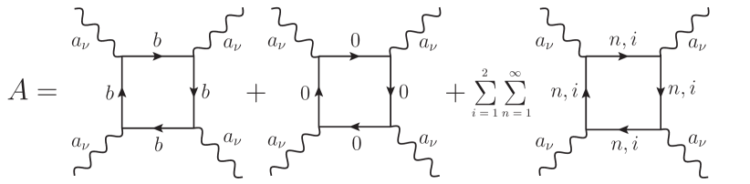
Figure 1: Diagrams corresponding to the $\gamma\gamma$ scattering amplitude. The number marking each fermion line corresponds to the number of the massive fermion Kaluza-Klein mode which is represented by the line. The letter $b$ stands for a brane-localized fermion.

For $\omega\ll m$, where $\omega$ is the energy of the photon in the c.m. frame, the regularized amplitude in the leading order in $\frac{\omega}{m}$ is given by [7]

$$A=\left(\frac{e^{4}\omega^{4}}{m^{4}}+\frac{e^{4}\omega^{4}}{M^{4}}+2\sum\limits_{n=1}^{\infty}\frac{e^{4}\omega^{4}}{\mu_{n}^{4}}\right)F(\theta),$$ (11)

where the function $F(\theta)$ depends on the scattering angle $\theta$ and the polarizations of the photons. We can estimate the series in $A$ using the standard Maclaurin-Cauchy integral test for convergence:

$$\frac{L}{4M^{3}}-\frac{L\arctan\left(\frac{\pi}{ML}\right)}{2\pi M^{3}}-\frac{L^{2}}{2M^{2}(\pi^{2}+M^{2}L^{2})}=\int_{1}^{\infty}dx\frac{L^{4}}{\left(\pi^{2}x^{2}+M^{2}L^{2}\right)^{2}}$$ (12)

$$<\sum\limits_{n=1}^{\infty}\frac{1}{\mu_{n}^{4}}=\sum\limits_{n=1}^{\infty}\frac{L^{4}}{\left(\pi^{2}n^{2}+M^{2}L^{2}\right)^{2}}<\int_{0}^{\infty}dx\frac{L^{4}}{\left(\pi^{2}x^{2}+M^{2}L^{2}\right)^{2}}=\frac{L}{4M^{3}}.$$

Thus, amplitude (11) can be estimated as

$$A>e^{4}\omega^{4}F(\theta)\left(\frac{1}{m^{4}}+\frac{1}{M^{4}}+\frac{L}{2M^{3}}-\frac{L\arctan\left(\frac{\pi}{ML}\right)}{\pi M^{3}}-\frac{L^{2}}{M^{2}(\pi^{2}+M^{2}L^{2})}\right).$$ (13)

One can see that in the limit $L\to\infty$, i.e., when we pass to an infinite extra dimension, the amplitude $A\to\infty$. Note that though the mass gaps between the Kaluza-Klein modes tend to zero in this limit, the mass gap $\Delta m=M-m$ between the brane-localized fermion and the lowest Kaluza-Klein mode remains intact, and it can be very large. A divergence of exactly the same type arises in the model discussed in [1]. This ”localization catastrophe” is the consequence of the fact that, though the vector field is localized on the brane, it interacts with the five-dimensional fermions everywhere in the bulk. Such a nonlocality of the interaction leads to a pathology, and it can arise in more realistic scenarios of gauge field localization on the brane.

It should be noted that the use of a finite cutoff scale does not solve the problem. Indeed, let us take a cutoff scale $\tilde{M}$ such that we do not take into account Kaluza-Klein modes with the masses $\mu_{n}>\tilde{M}$. The number of the heaviest Kaluza-Klein mode, which contributes to the amplitude, can be defined as $N=\lfloor\frac{L\sqrt{{\tilde{M}}^{2}-M^{2}}}{\pi}\rfloor$, where $\lfloor\cdot\rfloor$ stands for the floor function. Thus,

$$\sum\limits_{n=1}^{N}\frac{1}{\mu_{n}^{4}}>\sum\limits_{n=1}^{N}\frac{1}{{\tilde{M}}^{4}}=N\frac{1}{{\tilde{M}}^{4}}>\left(\frac{L\sqrt{{\tilde{M}}^{2}-M^{2}}}{\pi}-1\right)\frac{1}{{\tilde{M}}^{4}},$$ (14)

which tends to infinity in the limit $L\to\infty$ for $\tilde{M}>M$. Indeed, in the limit $L\to\infty$ the masses of the modes $\mu_{n}\to M$. Thus, the larger $L$ becomes, the greater the number of modes that appear below the cutoff scale $\tilde{M}$, each with the same coupling constant to the gauge field which does not depend on $L$, leading to an amplitude which increases with increasing $L$ (see also Appendix B for additional discussion of this issue). Formally, this problem can be solved by considering the cutoff scale such that some constant finite number of the modes $N_{f}$ is below the cutoff scale for any $L$. But in the limit $L\to\infty$, the corresponding cutoff scale $\tilde{M}_{f}\to M$, which is obviously unphysical. Moreover, in the limit $L\to\infty$, the discrete spectrum turns into the continuous one without isolated modes, and a fixed $N_{f}$ in this case means that the contribution from the continuous spectrum is of the measure zero — we just remove the continuous spectrum from the theory and do not estimate its contribution. So, here and below, we consider $\tilde{M}$ such that it does not depend on $L$, and $\tilde{M}>M$.

One can expect that effects analogous to the one which was demonstrated above can arise in other processes, such that the corresponding Feynaman diagrams contain the field $a_{\mu}$ in external lines and the fermion fields in internal lines. For example, let us take the polarization operator of the field $a_{\mu}$. The corresponding diagrams are presented in Figure 2.

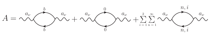
Figure 2: Diagrams which contribute to the polarization operator of the field $a_{\nu}$ in the leading order. As in Figure 1, the number marking each fermion line corresponds to the number of the massive fermion Kaluza-Klein mode which is represented by the line, and the letter $b$ stands for a brane-localized fermion.

The polarization operator has the form

$$\Pi_{\mu\nu}(q)=(q_{\mu}q_{\nu}-\eta_{\mu\nu}q^{2})\left(\Pi(q^{2},m_{b})+\Pi(q^{2},\mu_{0})+2\sum\limits_{n=1}^{\infty}\Pi(q^{2},\mu_{n})\right).$$ (15)

It is well known that for $q^{2}<m_{b}^{2}$ the function $\Pi(q^{2},m_{b})$ can be expanded as [8]

$$\Pi(q^{2},m_{b})=\Pi(0,m_{b})+\frac{\partial\Pi(q^{2},m_{b})}{\partial q^{2}}\biggl{|}_{q^{2}=0}q^{2}+\cdot\cdot\cdot,$$ (16)

where $\frac{\partial\Pi(q^{2},m_{b})}{\partial q^{2}}\bigl{|}_{q^{2}=0}=\frac{16i\pi^{2}}{60m_{b}^{2}}$, and $\Pi(0,m_{b})$ is logarithmically divergent. An analogous expansion can be made for the contributions of the other Kaluza-Klein fermions. Thus, in the leading order in $q^{2}/(\textrm{mass of the mode})^{2}$, the regularized contribution to the polarization operator is proportional to

$$q^{2}\left(\frac{1}{m_{b}^{2}}+\frac{1}{\mu_{0}^{2}}+2\sum\limits_{n=1}^{\infty}\frac{1}{\mu_{n}^{2}}\right).$$ (17)

In the limit $L\to\infty$, the sum in (17) also diverges. To show it, let us again introduce a cutoff scale $\tilde{M}>M$. In this case,

$$\sum\limits_{n=1}^{\infty}\frac{1}{\mu_{n}^{2}}>\sum\limits_{n=1}^{\lfloor\frac{L\sqrt{{\tilde{M}}^{2}-M^{2}}}{\pi}\rfloor}\frac{1}{\mu_{n}^{2}}>\sum\limits_{n=1}^{\lfloor\frac{L\sqrt{{\tilde{M}}^{2}-M^{2}}}{\pi}\rfloor}\frac{1}{{\tilde{M}}^{2}}=\frac{\lfloor\frac{L\sqrt{{\tilde{M}}^{2}-M^{2}}}{\pi}\rfloor}{{\tilde{M}}^{2}}>\left(\frac{L\sqrt{{\tilde{M}}^{2}-M^{2}}}{\pi}-1\right)\frac{1}{{\tilde{M}}^{2}}.$$ (18)

One can see that (18) indeed is divergent in the limit $L\to\infty$, so the polarization operator diverges for $q^{2}\neq 0$.

Just for a comparison, let us consider a rather different scenario — where the vector field can freely propagate in the bulk. In this case, the action for the vector field can be chosen to be

$$S_{vect}=-\int d^{4}xdz\frac{\xi^{2}}{4}F_{MN}F^{MN},$$ (19)

instead of the corresponding brane-localized term in (3). Here the constant $\xi$ with the dimension $\sqrt{\textrm{[mass]}}$ is introduced for convenience — the field $A_{M}$ in this case has the standard dimension [mass]. From the very beginning we can impose the gauge $A_{4}\equiv 0$. After imposing this gauge, we are left with the residual gauge transformations which are responsible for isolating the physical degrees of freedom of the massless four-dimensional vector field. We will be interested in the lowest mode of the vector field, so we take the ansatz $A_{\mu}(x,z)=\frac{1}{\xi\sqrt{2L}}a_{\mu}(x)$. Substituting it into action (19), integrating over the coordinate of the extra dimension, and taking into account (7) and (3), we obtain

$$S=\int d^{4}x\left.\Biggl{(}-\frac{1}{4}f_{\mu\nu}f^{\mu\nu}+i\bar{\psi}_{b}\gamma^{\mu}\left(\partial_{\mu}-ie_{4}a_{\mu}\right)\psi_{b}-m\bar{\psi}_{b}\psi_{b}\right.$$ (20)

$$\left.+i\bar{\psi}\gamma^{\mu}\left(\partial_{\mu}-ie_{4}a_{\mu}\right)\psi-M\bar{\psi}\psi+\sum\limits_{n=1}^{\infty}\sum\limits_{i=1}^{2}\left(i\bar{\psi}_{i}^{n}\gamma^{\mu}\left(\partial_{\mu}-ie_{4}a_{\mu}\right)\psi_{i}^{n}-\mu_{n}\bar{\psi}_{i}^{n}\psi_{i}^{n}\right)\right),$$

where $e_{4}=\frac{e}{\xi\sqrt{2L}}$.

Now let us calculate the amplitude corresponding to the process presented in Figure 1. It has the form

$$A=\left(\frac{e_{4}^{4}\omega^{4}}{m^{4}}+\frac{e_{4}^{4}\omega^{4}}{M^{4}}+2\sum\limits_{n=1}^{\infty}\frac{e_{4}^{4}\omega^{4}}{\mu_{n}^{4}}\right)F(\theta)=\frac{1}{4L^{2}\xi^{4}}\left(\frac{e^{4}\omega^{4}}{m^{4}}+\frac{e^{4}\omega^{4}}{M^{4}}+2\sum\limits_{n=1}^{\infty}\frac{e^{4}\omega^{4}}{\mu_{n}^{4}}\right)F(\theta).$$ (21)

Using (12) we can estimate the amplitude as

$$A<\frac{e^{4}\omega^{4}F(\theta)}{4\xi^{4}}\left(\frac{1}{L^{2}}\left(\frac{1}{m^{4}}+\frac{1}{M^{4}}\right)+\frac{1}{2M^{3}L}\right).$$ (22)

We see that now in the limit $L\to\infty$, the amplitude $A\to 0$. From the four-dimensional point of view, the only difference between this case and the previous one with the brane-localized gauge field is in the value of the coupling constant ($e$ versus $e/(\xi\sqrt{2L})$). From the physical point of view the difference is obvious — the second case corresponds to a local theory. Thus, in the limit $L\to\infty$, the zero mode of the gauge field $A_{\mu}$ ceases to be a four-dimensional particle — there is no mass gap between the zero mode and the next Kaluza-Klein mode of the vector field, and between the other Kaluza-Klein modes. Now all the Kaluza-Klein modes compose a single five-dimensional particle. In the resulting five-dimensional (though non-renormalizable in the usual sense) theory, the corresponding amplitude, of course, is nonzero.

Let us look at this case from another point of view — again by introducing the cutoff scale $\tilde{M}$. For the amplitude, we have

$$\sum\limits_{n=1}^{N}\frac{e_{4}^{4}}{\mu_{n}^{4}}<N\frac{e_{4}^{4}}{{M}^{4}}<\left(\frac{L\sqrt{{\tilde{M}}^{2}-M^{2}}}{\pi}-1\right)\frac{e^{4}}{4\xi^{4}L^{2}}\frac{1}{{M}^{4}},$$ (23)

which tends to zero when $L\to\infty$. Again, the larger $L$ becomes, the greater the number of modes that appear below the cutoff scale $\tilde{M}$, but now the effective coupling constant $e_{4}$ of each mode to the gauge field depends on $L$, leading to the amplitude which decreases with increasing $L$.

Finally, let us consider the last example — the model of quasilocalization of a gauge field proposed in [9] (a particular realization of this mechanism can be found in [10]). The action for the gauge field takes the form (in our notations)

$$S_{vect}=-\int d^{4}xdz\left(\frac{\xi^{2}}{4}F_{MN}F^{MN}+\delta(z)\frac{1}{4}F_{\mu\nu}F^{\mu\nu}\right).$$ (24)

As in the previous cases, let us put this system into a box in the extra dimension; i.e., let us suppose that the extra dimension forms an orbifold with the size $2L$. Again, we can impose the gauge $A_{4}\equiv 0$ and expand the vector field into Kaluza-Klein modes. The lowest mode (which we will be interested in) of the vector field has a constant wave function in the extra dimension (which follows from the corresponding equations of motion for the vector field), so we can take the ansatz $A_{\mu}(x,z)=\frac{1}{\sqrt{2\xi^{2}L+1}}a_{\mu}(x)$. After substituting it into (24), integrating over the coordinate of the extra dimension, and taking into account (6), we obtain (20), but now with $e_{4}=\frac{e}{\sqrt{2\xi^{2}L+1}}$. Instead of (23), we get

$$\sum\limits_{n=1}^{N}\frac{e_{4}^{4}}{\mu_{n}^{4}}<N\frac{e_{4}^{4}}{{M}^{4}}<\left(\frac{L\sqrt{{\tilde{M}}^{2}-M^{2}}}{\pi}-1\right)\frac{e^{4}}{\left(2\xi^{2}L+1\right)^{2}}\frac{1}{{M}^{4}},$$ (25)

which also tends to zero when $L\to\infty$. As in the previous case with the gauge field living in the bulk, in the limit $L\to\infty$, the zero mode of the gauge field $A_{\mu}$ ceases to be a four-dimensional particle — there is no mass gap between the zero mode and the next Kaluza-Klein mode of the vector field, and between the other Kaluza-Klein modes (this happens because of the existence of the term $\frac{\xi^{2}}{4}F_{MN}F^{MN}$ in (24)). Again, we cannot isolate the purely four-dimensional massless photon (a localized zero mode is absent in such a scenario — the photon behaves as a four-dimensional particle at small distances, whereas at large distances it possesses a five-dimensional behavior; see [9] for details), contrary to the case of the localized gauge field described by equations (3) and (6), where the mass gap between the lowest localized mode and the rest Kaluza-Klein tower (which can be taken into account by adding (10) to (3) and (6)) remains nonzero even in the limit $L\to\infty$, in full analogy with [1].

An interesting observation is that (24) turns into the boson part of (3) if one takes $\xi=0$. But the choice $\xi=0$ means that there is a strong coupling outside the brane in our toy model (this also follows from the five-dimensional action in (1) — the ”coupling constant” $\frac{1}{\sqrt{G(z)}}$ grows with $z$). It is obvious that this strong coupling is directly connected to the divergences discussed above.

In conclusion, we have considered the simplest case of an Abelian gauge field. It was shown that the localization of such a gauge field on a brane can result in an effective action (as an example, one can consider the model discussed in [1]) analogous to those coming from multidimensional theories containing nonlocal interactions from the very beginning. Since one may expect pathologies in theories with nonlocal interactions, analogous pathologies can arise in theories with brane-localized gauge fields in more general cases. One should take this effect into account when considering brane world models with infinite extra dimensions.

Appendix A

According to the orbifold symmetry conditions (4) and (5), the five-dimensional fermion fields $\Psi_{1}$ and $\Psi_{2}$ can be decomposed into Kaluza-Klein modes (see [6]) as

$$\Psi_{1}(x,z)=\frac{1}{\sqrt{2L}}\psi_{L}(x)+\frac{1}{\sqrt{L}}\sum\limits_{n=1}^{\infty}\left(\cos\left(\frac{\pi n}{L}z\right)\psi^{n}_{L}(x)-\sin\left(\frac{\pi n}{L}z\right)\hat{\psi}^{n}_{R}(x)\right),$$ (26)

$$\Psi_{2}(x,z)=\frac{1}{\sqrt{2L}}\psi_{R}(x)+\frac{1}{\sqrt{L}}\sum\limits_{n=1}^{\infty}\left(\cos\left(\frac{\pi n}{L}z\right)\psi^{n}_{R}(x)+\sin\left(\frac{\pi n}{L}z\right)\hat{\psi}^{n}_{L}(x)\right),$$ (27)

where $\psi_{L}(x)=\gamma^{5}\psi_{L}(x)$, $\psi_{R}(x)=-\gamma^{5}\psi_{R}(x)$, $\psi^{n}_{L}(x)=\gamma^{5}\psi^{n}_{L}(x)$, $\psi^{n}_{R}(x)=-\gamma^{5}\psi^{n}_{R}(x)$, $\hat{\psi}^{n}_{L}(x)=\gamma^{5}\hat{\psi}^{n}_{L}(x)$, $\hat{\psi}^{n}_{R}(x)=-\gamma^{5}\hat{\psi}^{n}_{R}(x)$. Substituting (26) and (27) into (6) and integrating over the coordinate $z$ of the extra dimension, we arrive at

$$S_{f\_eff}=\int d^{4}x\left[i\bar{\psi}\gamma^{\mu}\left(\partial_{\mu}-iea_{\mu}\right)\psi-M\bar{\psi}\psi+\sum\limits_{n=1}^{\infty}\left.\Bigl{(}i\bar{\psi}^{n}\gamma^{\mu}\left(\partial_{\mu}-iea_{\mu}\right)\psi^{n}\right.\right.$$ (28)

$$\left.\left.+i\bar{\hat{\psi}}^{n}\gamma^{\mu}\left(\partial_{\mu}-iea_{\mu}\right)\hat{\psi}^{n}-\frac{\pi n}{L}(\bar{\hat{\psi}}^{n}\psi^{n}+\bar{\psi}^{n}\hat{\psi}^{n})-M(\bar{\psi}^{n}\psi^{n}-\bar{\hat{\psi}}^{n}\hat{\psi}^{n})\right)\right.\Biggr{]}$$

with

$$\psi(x)=\psi_{L}(x)+\psi_{R}(x),$$ (29)

$$\psi^{n}(x)=\psi_{L}^{n}(x)+\psi_{R}^{n}(x),$$ (30)

$$\hat{\psi}^{n}(x)=\hat{\psi}_{L}^{n}(x)+\hat{\psi}_{R}^{n}(x).$$ (31)

We see that the mass matrix is nondiagonal. In order to bring it into a diagonal form, we use the transformations

$$\psi^{n}(x) = \psi_{1}^{n}(x)\cos(\theta_{n})+\psi_{2}^{n}(x)\sin(\theta_{n}),$$ (32)

$$\hat{\psi}^{n}(x) = \psi_{1}^{n}(x)\sin(\theta_{n})-\psi_{2}^{n}(x)\cos(\theta_{n})$$ (33)

with

$$\tan(2\theta_{n})=\frac{\pi n}{ML}$$ (34)

and obtain

$$S_{f\_eff}=\int d^{4}x\left[i\bar{\psi}\gamma^{\mu}\left(\partial_{\mu}-iea_{\mu}\right)\psi-M\bar{\psi}\psi+\sum\limits_{n=1}^{\infty}\left(i\bar{\psi}_{1}^{n}\gamma^{\mu}\left(\partial_{\mu}-iea_{\mu}\right)\psi_{1}^{n}\right.\right.$$ (35)

$$\left.\left.+i\bar{\psi}_{2}^{n}\gamma^{\mu}\left(\partial_{\mu}-iea_{\mu}\right)\psi_{2}^{n}-\mu_{n}(\bar{\psi}_{1}^{n}\psi_{1}^{n}-\bar{\psi}_{2}^{n}\psi_{2}^{n})\right)\right.\Biggr{]},$$

where $\mu_{n}=\sqrt{\frac{\pi^{2}n^{2}}{L^{2}}+M^{2}}$. We see that the mass terms of the fields $\psi_{2}^{n}$ have unconventional signs. But with the help of the standard redefinition $\psi_{2}^{n}\to\gamma^{5}\psi_{2}^{n}$, we can bring the action of (35) into the standard form of (7).

It should be noted that one can find a similar doubling of the number of four-dimensional effective degrees of freedom in the case of one five-dimensional massive fermion in a space-time with one compact extra dimension, where the extra dimension does not possess the orbifold symmetry. Thus, the number of effective four-dimensional degrees of freedom in the case of two five-dimensional fermions in a space-time with a compact extra dimension forming the $S^{1}/Z_{2}$ orbifold — and in the case of a single five-dimensional fermion in a space-time with a compact extra dimension without the orbifold symmetry — is the same; i.e., the existence of the orbifold symmetry reduces almost by half the number of Kaluza-Klein modes coming from each five-dimensional fermion.

Appendix B

Suppose the size of the extra dimension is rather large: $ML\gg 1$. In this case, the mass gap between two successive modes takes the form

$$\Delta\mu_{n}=\mu_{n+1}-\mu_{n}\approx\frac{\mu_{n+1}^{2}-\mu_{n}^{2}}{2\mu_{n}}=\frac{\pi^{2}(2n+1)}{2L^{2}\mu_{n}}=\frac{\pi}{L\mu_{n}}\left(\sqrt{\mu_{n}^{2}-M^{2}}+\frac{\pi}{2L}\right),$$ (36)

where we have used equation (8). Now we can rewrite the first term of (14) as

$$\sum\limits_{n=1}^{N}\frac{1}{\mu_{n}^{4}}=\sum\limits_{n=1}^{N}\frac{\Delta\mu_{n}}{\Delta\mu_{n}}\frac{1}{\mu_{n}^{4}}\approx\sum\limits_{n=1}^{N}\frac{L\Delta\mu_{n}}{\pi\mu_{n}^{3}\left(\sqrt{\mu_{n}^{2}-M^{2}}+\frac{\pi}{2L}\right)}\approx\frac{L}{\pi}\int_{M}^{\tilde{M}}\frac{d\mu}{\mu^{3}\left(\sqrt{\mu^{2}-M^{2}}+\frac{\pi}{2L}\right)}.$$ (37)

For any fixed cutoff scale $\tilde{M}>M$, the integral in (37) is finite. The larger $L$ becomes, the better the integral term in (37) approximates the initial sum. In the limit $L\to\infty$, the integral itself remains finite, but due to the factor $L$ in front of it, the amplitude tends to infinity.

Integrals analogous to the one in (37) are expected to arise in models with infinite extra dimension. But the origin of the factor $L$ in front of the integral in (37) is not obvious. Below, we will show schematically how it arises in a model with initially infinite extra dimension. Indeed, the existence of a continuous spectrum of excitations in effective four-dimensional theory implies that there is a five-dimensional particle which can move along the extra dimension. It possesses a momentum $p^{z}$ along the extra coordinate $z$, varying in the limits $M\leq p^{z}\leq\tilde{M}$, where the upper limit is defined by our choice of the cutoff scale (of course, in the general case, the particle can move in the opposite direction; i.e., we should also take $-M\geq p^{z}\geq-\tilde{M}$, but it is irrelevant for our analysis). Now let us consider the $\gamma\gamma\to\gamma\gamma$ scattering process, but with the five-dimensional particle in the internal lines instead of a set of four-dimensional particles; see Figure 3.

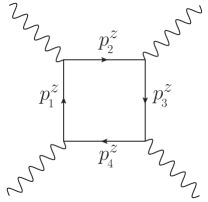
Figure 3: Diagram corresponding to the $\gamma\gamma$ scattering amplitude with five-dimensional particles in internal lines. $p^{z}_{i}$, where $i=1,...,4$; stand for the momenta of the five-dimensional fermions in the extra dimension.

The corresponding matrix element contains a term of the form

$$\int dp^{z}_{1}\int dp^{z}_{2}\int dp^{z}_{3}\int dp^{z}_{4}\,\delta(p^{z}_{1}-p^{z}_{2})\delta(p^{z}_{2}-p^{z}_{3})\delta(p^{z}_{3}-p^{z}_{4})\delta(p^{z}_{4}-p^{z}_{1})F(p^{z}_{1},p^{z}_{2},p^{z}_{3},p^{z}_{4}),$$ (38)

where $F(p^{z}_{1},p^{z}_{2},p^{z}_{3},p^{z}_{4})$ is a function depending on the momenta of fermions in internal lines in the extra dimension [for simplicity, the four-dimensional momenta of particles in external and internal lines of the diagram in Figure 3, together with the corresponding integrals, are included in the definition of the function $F(p^{z}_{1},p^{z}_{2},p^{z}_{3},p^{z}_{4})$]. Note that localized photons do not carry momenta in the extra dimension; i.e., we cannot say that a localized four-dimensional photon is just a five-dimensional particle with $p^{z}=0$ — that is why $\delta$ functions in (38) contain momenta in the extra dimension only of the five-dimensional fermions. The integrals in (38) can be easily evaluated, and we get

$$\int_{M}^{\tilde{M}}dp^{z}_{1}\,\delta(p^{z}_{1}-p^{z}_{1})F(p^{z}_{1},p^{z}_{1},p^{z}_{1},p^{z}_{1})=\delta(0)\int_{M}^{\tilde{M}}dp^{z}_{1}\,F(p^{z}_{1},p^{z}_{1},p^{z}_{1},p^{z}_{1}).$$ (39)

Though the integral on the RHS of (39) can be finite (at least after a four-dimensional regularization), the value of (39) is infinite because of the factor $\delta(0)$. But $\delta(0)=\frac{1}{2\pi}\int_{-\infty}^{\infty}dz=\frac{L}{\pi}$ (where $L\to\infty$), which is nothing but the size of the extra dimension. Thus, we have demonstrated how the factor $L$ arises in model with initially infinite extra dimension.

References

- [1] M.N. Smolyakov, Phys. Rev. D 85 (2012) 045036, Erratum-ibid. D 87 (2013) 029901.
- [2] V. A. Rubakov and M. E. Shaposhnikov, Phys. Lett. B 125 (1983) 136.
-
[3]
S.L. Dubovsky, V.A. Rubakov and P.G. Tinyakov, Phys. Rev. D
62 (2000) 105011.
M.V. Libanov and S.V. Troitsky, Nucl. Phys. B 599 (2001) 319.
R. Casadio and A. Gruppuso, Phys. Rev. D 64 (2001) 025020.
A.A. Andrianov, V.A. Andrianov, P. Giacconi and R. Soldati, JHEP 0307 (2003) 063.
A.A. Andrianov, V.A. Andrianov, P. Giacconi and R. Soldati, JHEP 0507 (2005) 003. -
[4]
A. Kehagias and K. Tamvakis, Phys. Lett. B 504 (2001)
38.
M.E. Shaposhnikov and P. Tinyakov, Phys. Lett. B 515 (2001) 442.
A.T. Barnaveli and O.V. Kancheli, Sov. J. Nucl. Phys. 52 (1990) 576. - [5] V.A. Rubakov, Phys. Usp. 44 (2001) 871.
- [6] C. Macesanu, Int. J. Mod. Phys. A 21 (2006) 2259.
- [7] A.I. Akhiezer, V.B. Berestetskii, Quantum Electrodynamics (Interscience Publishers, New York, 1965).
- [8] S.S. Schweber, An Introduction to Relativistic Quantum Field Theory (Row, Peterson and Co, Evanston, 1961).
- [9] G.R. Dvali, G. Gabadadze and M. A. Shifman, Phys. Lett. B 497 (2001) 271.
- [10] C. Germani, Phys. Rev. D 85 (2012) 055025.
-
[11]
D. Binosi, L. Theussl, Comput. Phys. Commun. 161 (2004)
76.
D. Binosi, J. Collins, C. Kaufhold, L. Theussl, Comput. Phys. Commun. 180 (2009) 1709.