Threat, support and dead edges in the Shannon game

Abstract

The notions of captured/lost vertices and dead edges in the Shannon game (Shannon switching game on nodes) are examined using graph theory. Simple methods are presented for identifying some dead edges and some captured sets of vertices, thus simplifying the (computationally hard) problem of analyzing the game.

1 Introduction

In the Shannon game two vertices in a simple graph are designated as terminals, and one player aims to link the terminals, the other to prevent this, by colouring vertices. This is of interest both in its own right as a mathematical problem in graph theory and because of its connection to the theory of robust networks and fault-tolerance. An understanding of the game can elucidate more general problems, such as the Shannon game with more terminals (discussed below) or with terminals that can change. Various hard computational problems arise in aspects of the game, see [1] for a review.

It was shown by Björnsson et al. [2] that analysis of the Shannon game can be simplified by considering local games (played on a subgraph) as long as the complete neighbourhood of the subgraph is considered, yielding a type of Shannon game with multiple terminals, called a multi-Shannon game (defined in [2] and below). They introduced a concept of domination, relating to the winner of a multi-Shannon game, and presented a set of local patterns in the game Hex where empty cells could be filled in without changing the outcome of the game.

In this paper we introduce concepts related to domination (in the sense of Björnsson et al.), but which are defined in terms of easily identifiable properties of a graph. This simplifies the analysis and permits a number of theorems concerning multi-Shannon games to be easily stated and proved. All the local Hex patterns considered in [2] can be detected through simple graph properties such as counting small walks and triangles. We also discuss the concept of a dead edge, defined in section 5, and present theorems to help identify dead edges. Some further theorems allowing won or lost patterns to be detected are also obtained.

2 Game definition

The Shannon game is played on any simple graph (i.e. no self-loops and no multiple edges), with two of the vertices designated terminals. One player (called Short) seeks to join the terminals, the other (called Cut) seeks to prevent this. Shannon originally proposed colouring edges of the graph, i.e. in each turn Short can colour one edge, and Cut can delete one uncoloured edge. This version is known as the Shannon switching game; it has a polynomial-time algorithmic solution [3]. In this paper we consider only the Shannon switching game on nodes, known as the Shannon game. In the Shannon game, in each turn Short can colour one vertex, and Cut can delete one uncoloured vertex. Short has won if there exists a path between the terminals consisting only of coloured vertices; Cut  has won if the graph is disconnected with the terminals in different components. It is obvious that a draw is not possible.

Instead of deleting vertices Cut may equivalently colour vertices a different colour to Short (e.g. Short is black and Cut is white), then Cut has won if there is a cutset separating the terminals consisting of all white vertices. We will call this the graph colouring model of the game.

The game Hex can be considered as a (beautiful and fascinating) example of the Shannon game, played on a finite planar graph corresponding to an $m\times m$ honey-comb lattice of hexagonal cells (vertices in the graph are adjacent when their corresponding cells are adjacent), with two further vertices (the terminals) adjacent to all vertices on each of two opposite sides of the lattice [1]. If we choose to define the rules of Hex such that one player has to connect the designated sides and the other has to prevent this, then the correspondence to the Shannon game is direct and obvious. However, the rules of Hex are conventionally stated another way: both players colour vertices (with different colours) and one player has to connect one pair of sides, the other player the other pair of sides. That the latter version (standard Hex rules) is equivalent to the former (Shannon game)—i.e. that joining one pair of sides in Hex is equivalent to separating the other pair of sides—was shown by Beck [4] and Gale [5], see also [1].

The Shannon game as described above, where in each turn Short colours a vertex, can also be modelled another way, in which whenever Short picks a vertex $v$, edges are added to the graph between all pairs of neighbours of $v$ which are not already adjacent, and then $v$ is deleted. We refer to this as the reduced graph model. It is easy to see that the graph colouring and reduced graph models are equivalent. Most of the proofs in this paper use the reduced graph model.

The reduced graph model shows that any position in the course of a Shannon game is equivalent to an opening position on a smaller graph (i.e. one with fewer vertices; the number of edges may grow or shrink). Such a position is uniquely specified by the reduced graph, the terminal pair designation and identity of the player who is to move next: $(G,\{t_{1},t_{2}\},P)$. In this paper the Roman font symbol $G$ will always refer to a reduced graph, and we will usually suppress the terminal designation in order to reduce clutter (the terminal designation does not change during the game). For convenience we assign binary values to the players, $P=1$ for Short and $P=0$ for Cut, so if a given player is $P$, then the other player is $\neg P$.

Lemma 1

For every position in the Shannon game, one of the players has a winning strategy.

This is well known and follows from elementary game theory, but it is essential in the following so we exhibit a proof, by induction: Let $(G_{n},P)$ describe the position when the reduced graph has $n$ vertices, the player to move is $P$, and we suppressed the terminal designation. We assume that for every possible position of size $n-1$ which is reachable from $(G_{n},P)$, one of the players (not necessarily the same for all the graphs) has a winning strategy. If among this set there is a position $(G_{n-1},\neg P)$ for which $P$ has a winning strategy, then $P$ has a winning strategy for $(G_{n},P)$. If not, then all the $\{(G_{n-1},\neg P)\}$ reachable from $(G_{n},P)$ give a winning strategy for $\neg P$, from which it follows that $\neg P$ has a winning strategy for $(G_{n},P)$. This establishes the inductive step. It remains to prove the case for some low $n$, and this follows immediately from the fact that $n$ falls as the game proceeds, and ultimately the game is won or lost (not drawn).

The analysis of the Shannon game has two main aims: to identify the winner for a general position, and to find a winning strategy.

Determining the winner of a general Hex position has been shown to be PSPACE-complete [6], and therefore so is the solution of the Shannon game.

2.1 Notation and terminology

We will use the term ‘graph’ to signify a simple graph with two special vertices (the terminals), i.e. $G=(V,E,\{t_{1},t_{2}\})$ is a simple graph with vertex set $V$, edge set $E$, terminal set $\{t_{1},t_{2}\}\subset V$. A position $(G,P)$ is a graph (having designated terminals) with an indication $P$ of which player is to play next.

A clique is a set of vertices each adjacent to all the others in the set. In standard graph terminology the term means a maximal such set. In this paper it will not be important whether the set is maximal or non-maximal (i.e. a subset of a maximal clique). We will use ‘clique’ to mean a vertex set which is either a non-maximal clique or a (maximal) clique.

$G-v$ means the graph obtained from $G$ by deleting vertex $v$. $G\ast v$ means the graph obtained from $G$ by shorting vertex $v$, that is, adding edges between all non-adjacent pairs in the neighbourhood of $v$ (converting the neighbourhood into a clique), and then deleting $v$. Note that in both cases the vertex is deleted. These two operations commute when applied to two different vertices (this is obvious from the graph colouring model). It is not possible to apply them successively to the same vertex. For an edge $e$, $G+e$ means the graph obtained by adding edge $e$, $G-e$ means the graph obtained by deleting edge $e$.

If $S$ is a set vertices, then $G-S$ means the graph obtained by deleting the members of $S$ and $G*S$ means the graph obtained by shorting the members of $S$.

Terminals may never be deleted or shorted.

The open neighbourhood of a vertex $v$ is denoted $\Gamma(v)$. The closed neighbourhood is denoted $\Gamma[v]\equiv\Gamma(v)\cup\{v\}$. Define the neighbourhood $\Gamma(S)$ of a set of vertices $S$ to be the set of vertices not in $S$ but adjacent to a member of $S$: $\Gamma(S)\equiv(\cup_{v\in S}\Gamma(v))\setminus S$, where $\setminus$ is the set minus operation.

If $a\in S$ then we use the shorthand $S-a\equiv S\setminus\{a\}$.

The triangle number $T(v)$ is the number of triangles containing vertex $v$.

The win-value $W(G,P)$ of a position is the identity of the player holding a winning strategy.

3 Multi-Shannon game: domination, capture and loss

The multi-Shannon game is introduced in [2] in order to define concepts and methods useful to solving the Shannon game. In this section we present the game definition, quote the main result of [2], and present some new results.

If $S$ is a set of vertices in a graph $G$ then a multi-Shannon game is played on the induced subgraph $G(S\cup\Gamma(S))$ with the vertices $S$ as ‘playing area’ and the vertices $\Gamma(S)$ designated as ‘terminals’. There may be any number of terminals.

To describe the game it is convenient to use both the graph colouring model and the reduced graph. Short seeks to play in such a way that at the end of the game, when all vertices in $S$ have been coloured, the reduced graph (which, at the end, consists only of terminals and possibly edges between them) is the same as would be obtained if all of $S$ had been shorted. Cut seeks to play in such a way that the outcome (i.e. the final reduced graph among terminals) is the same as if all of $S$ had been cut. If neither eventuality occurs, then the game is drawn. (If both occur, because, for example, the terminals were all mutually adjacent at the start, then both players may declare a win; the vertices in $S$ are then ‘dead’, a concept we will discuss later).

The above rule definition clears up a slight ambiguity in [2] for the case where the graph was not connected at the outset. If the graph is connected then a Short win turns the reduced graph terminals into a clique. If the terminals initially had no edges between them then a Cut win turns the reduced graph terminals into a set of isolated vertices. In the graph colouring model, Short is trying to make Short-coloured paths between all connected but non-adjacent terminal pairs, and Cut is trying to occupy cutsets that separate all non-adjacent terminal pairs.

The multi-Shannon game is useful because it offers a way to simplify the analysis of the regular Shannon game, by reducing part of the complete game to a local ‘battle’, as follows. Consider any set $S$ of non-terminal vertices of the reduced graph in a Shannon game. Let ${\cal M}_{G,S}$ be the multi-Shannon game played on the subgraph of $G$ induced by $S\cup\Gamma(S)$ with terminals $\Gamma(S)$.

Definition $S$ is captured in $G$ if Short has a second-player winning strategy for ${\cal M}_{G,S}$. $S$ is lost in $G$ if Cut has a second-player winning strategy for ${\cal M}_{G,S}$.

Theorem 1

(Björnsson, Hayward, Johanson, van Rijswijck) If $S$ is captured, then $W(G,x)=W(G\ast S,x)\forall x$. If $S$ is lost, then $W(G,x)=W(G-S,x)\forall x$.

Proof: see [2]. Our terminology ‘captured’ and ‘lost’ reflects the point of view of Short. The same concept is referred to in [2] as ‘captured by short’ and ‘captured by cut’.

Observe that in the first case, to solve $G$, it suffices to solve $G\ast S$, and in the second case, to solve $G$, it suffices to solve $G-S$. In either case the resulting problem is usually simpler because the reduced graph has fewer vertices. Therefore when vertices are captured (lost) one may as well go ahead and short (cut) them as a ‘free move’ in order to clarify matters. This is called ‘filling in’ in discussions of Hex [1]. To be clear in the following one should note that to be captured or lost is strictly a property of a set of vertices (in a given graph) rather than of the members of the set. For example a captured set can be a subset of a lost set, and vice versa, see figure 1 for examples.

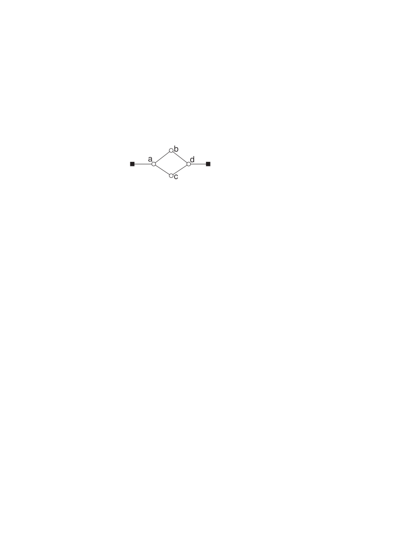
Figure 1: Examples of capture and loss. The filled squares are terminals. $\{b,c\}$ is captured but $\{a,b,c,d\}$ is lost.

Definition $S$ is $P$-dominated if $P$ has a first-player winning strategy for ${\cal M}_{G,S}$. For any initial move $v$ in such a strategy, we say that $v$ $P$-dominates $S$.

The terminology here is precisely as in [2]. Domination is a property of a set as a whole: if a set $S$ is $P$-dominated it does not necessarily follow that a subset $U\subset S$ is $P$-dominated. For example figure 2 shows a case where $a$ cut-dominates $\{a,b,c\}$ but $a$ does not cut-dominate $\{a,b\}$ or $\{a,c\}$.

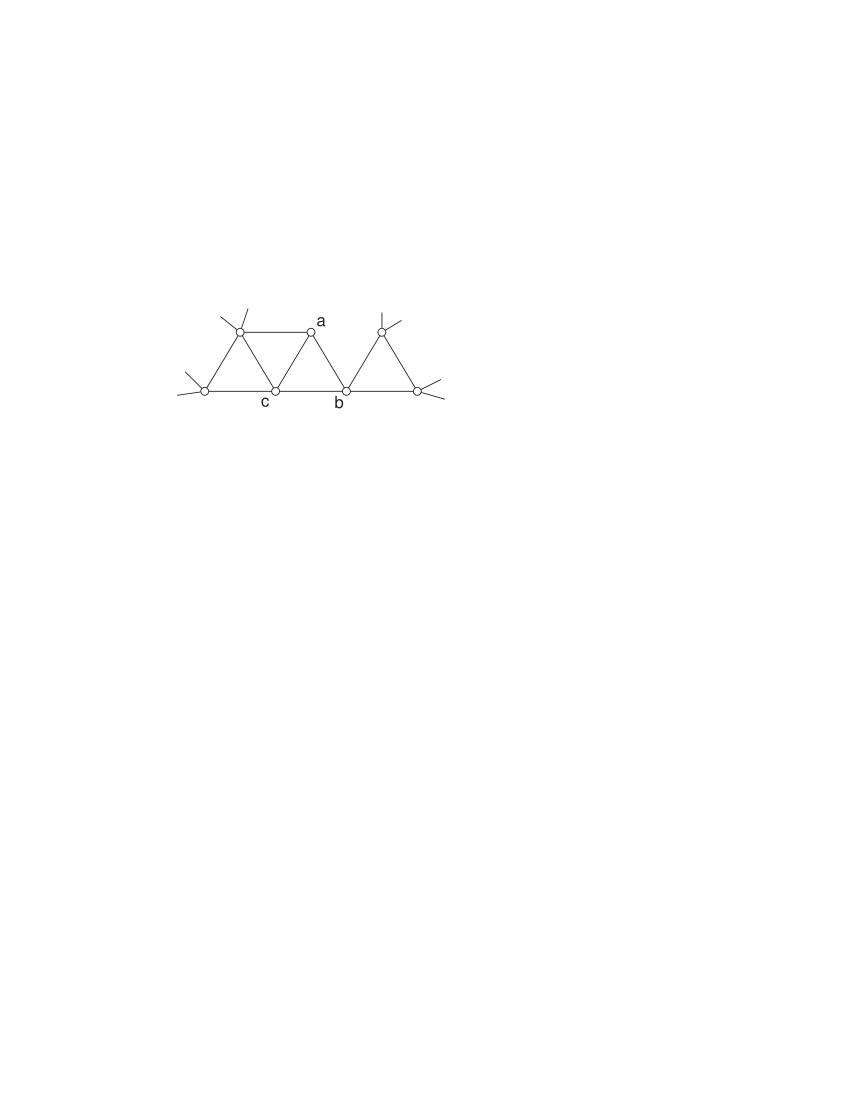
Figure 2: Examples of cut-domination. The diagram shows part of a larger graph; edges attached to only one vertex are used to signify that the vertex may have further neighbours which are irrelevant to the point under discussion. In this example, $b$ cut-dominates $\{a,b\}$ because after deleting $b$ the neighbourhood of $a$ becomes a clique. $a$ cut-dominates $\{a,b,c\}$ because if $a$ is deleted then $b$ and $c$ become a lost pair (c.f. figure 3(a)). However, $a$ does not cut-dominate $\{a,b\}$ or $\{a,c\}$. (The edge $ac$ is dead, see theorem 14).

Simple examples . If $G-a\ast b-c=G-a-b\ast c=G-a-b-c$ then $a$ cut-dominates $\{a,b,c\}$ (c.f. figure 2); if $G\ast a\ast b-c=G\ast a-b\ast c=G\ast a\ast b\ast c$ then $a$ short-dominates $\{a,b,c\}$.

Theorem 2

If both vertices in a two-vertex set $P$-dominate the set, then both are captured, lost respectively for $P$=Short, Cut.

(This property was noted in [2]). Proof: in the multi-Shannon game played on these two vertices, after the opening move by $\neg P$, there is only one response for $P$ and then the game is over, with a final position exactly the same as if $P$ had opened (with a winning move) and $\neg P$ replied. $\Box$

Simple examples (See figure 3). Two neighbouring vertices both of degree 2 are lost, unless one or both is terminal. For two vertices of degree 2 having the same neighbours, if neither is terminal then both are captured; if one is terminal then the other is dead (see later); if both are terminal then the game is won by Short.

Figure 3: Examples of mutually dominating pairs. (a) The dotted vertices cut-dominate each other and therefore are lost. (b) The dotted vertices short-dominate each other and therefore are captured.

N.B. This theorem is concerned with pairs not larger sets. It states for example that if $a$ cut-dominates $\{a,b\}$ and $b$ cut-dominates $\{a,b\}$ then $a$ and $b$ are lost. However, if $a$ cut-dominates $\{a,b,c\}$ and $b$ cut-dominates $\{a,b\}$ it does not necessarily follow that $\{a,b\}$ is lost: figure 2 gives a counter-example.

Theorem 3

If each of two vertices in a three-vertex set $P$-dominate the set, then so does the third.

Proof: let $1$ and $0$ stand for moves by $P$ and $\neg P$. There are three possible outcomes after three moves in a three-vertex multi-Shannon game when $P$ goes first: $110,\,101,\,011$ (in an obvious notation). If the first vertex $P$-dominates the set then both $110$ and $101$ must be $P$-wins because $\neg P$ can force either of these positions after a $P$ opening at the first vertex. Similarly, if the second vertex $P$-dominates the set then both $110$ and $011$ must be $P$-wins. Hence $101$ and $011$ are both $P$-wins, and therefore the third vertex also $P$-dominates the set. $\Box$

For example, in figure 2 $a$ and $b$ both cut-dominate $\{a,b,c\}$, therefore so does $c$.

Theorem 4

If each of two vertices in a four-vertex set $P$-dominate the set, but occupying them both is not a winning strategy for $P$, then $P$ has a second-player winning strategy for the multi-Shannon game on this set.

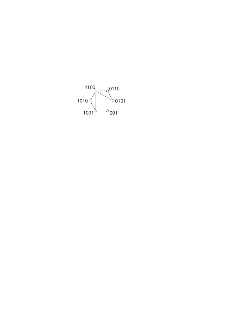
Figure 4: A graph indicating possible outcomes of a game on a 4-vertex set considered in theorem 4.

Proof: let the vertices be labeled $a,b,c,d$ with $a$ and $b$ $P$-dominating the set. There are six possible final positions, namely $1100,1010,1001,0110,0101,0011$, where we list the vertex colours in the order $abcd$. Suppose first that $P$ moves first, and occupies vertex $a$. Since $a$ $P$-dominates the set, this is a winning move, which implies that for each of the three replies available to $\neg P$, $P$ can still obtain a won final position. This means that $P$ must win at least one of $1010,1001$ (the available outcomes if $\neg P$ replies at $b$), and at least one of $1100,1001$ and at least one of $1100,1010$. These pairs are indicated by three of the edges of the graph shown in figure 4. Now suppose that $P$ moves first and occupies vertex $b$. Since $b$ $P$-dominates the set, this is also a winning move and by similar reasoning we conclude that $P$ wins at least one of each of the three pairings indicated by the remaining edges in figure 4.

Let us call the graph shown in figure 4 the win-graph. Next consider the win-values of each of the final positions. For each edge in the win-graph, at least one vertex to which it is incident is a won position for $P$. In other words, the won positions form a vertex-cover of the win-graph. However, the conditions of the theorem assert that $1100$ is not winning for $P$. It follows that $1010,1001,0110,0101$ are all won by $P$. Therefore the only way for $\neg P$ to win or draw is to realise one of $1100$ or $0011$. However, after any opening move by $\neg P$, the reply by $P$ can guarantee to avoid both of those outcomes. Hence $P$ must win. $\Box$

The general relationship between capture/loss and domination is obvious: $P$ has a second-player winning strategy if and only if $P$ has a first-player winning strategy after any opening move by $\neg P$. For the case of Short this general idea can be simplified, as follows.

Theorem 5

$S$ is captured if and only if Short has 1st-player winning strategies for ${\cal M}_{G,S}$ on each of a set of subsets of $S$ having empty total intersection.

By “subsets having empty total intersection” we mean $\{U_{i}\}:U_{i}\subset S,U_{1}\cap U_{2}\cap\ldots U_{m}=\emptyset$, where $m$ is the number of subsets. A winning strategy for $P$ “on a subset” means that the strategy involves play (by either player) only within the subset. To prove such a strategy on a subset for Short, it suffices to consider the subgraph induced by the subset plus $\Gamma(S)$ (i.e. the terminals of ${\cal M}_{G,S}$, not the neighbourhood of the subset under consideraton), and this means the theorem serves as a useful way to break down the task of finding 2nd-player winning strategies for Short. The subsets useful for Short are those which connect to all the terminals and which are well-connected internally. We will explain in a moment why there is no straightforwardly analogous theorem for Cut.

Proof. ($\Leftarrow$) Cutting vertices outside a given subset does nothing to the graph induced by that subset, and the empty total intersection implies that after the opening move by Cut, at least one Short-winning subset has not been intruded upon. Short plays the 1st-player winning strategy for any one such subset. ($\Rightarrow$) If Short has a 2nd-player winning strategy, then by definition he has a 1st-player winning strategy after any opening move $v$ by Cut, and that move did not affect the subgraph induced by $U_{v}=S-v$. Therefore the set of subsets $\{U_{v}\}\forall v\in S$ is one possible set satisfying the theorem. $\Box$

When one tries to break down the task of Cut into sub-games, the situation is less straightforward, because ruling out the existence of any path is more complicated than establishing the existence of one path. We already noted that Cut has a 2nd- player winning strategy if and only if he has a 1st-player winning strategy after any opening move by Short, but one would like to identify a way to reduce the problem further. One possibility is to look for a smaller multi-Shannon game (a sub-game of the one under consideration) which has a 1st-player strategy for Cut to win outright, but there does not necessarily exist any such sub-game. One cannot simply adapt theorem 5 to Cut’s case, for two main reasons. First, to prove that Cut can prevent paths useful to Short from forming within a given vertex set $U$, it is not sufficient to consider the induced subgraph $G(U\cup\Gamma(S))$, because shorting vertices outside of $U$ can add edges to $G(U)$. Secondly, if it is to be sufficient for Cut to have first-player wins on each of a set of subsets, then the subsets must be arranged in series rather than in parallel, that is, nested in such a way that every path between non-neighbour terminals passes through sufficiently many subsets. However, the property of whether a given subset $U\subset S$ is thus in series with the rest is not a property of $U$ alone: it is a property of the whole set. This is in contrast with the subsets sought by Short: the property that a given subset $U$ connects all terminals $T=\Gamma(S)$ in a multi-Shannon game (i.e. $T\subset\Gamma(U)$) is a property of the induced subgraph $G(U\cup T)$ alone, without regard to the rest of the graph.

Theorem 5 is reminiscent of the ‘or-rule’ recognized by all early exponents of the game of Hex and investigated more fully by Anshelevich [7, 8]. The standard ‘or-rule’ is concerned with ‘virtual connections’ or ‘links’ between a given pair of vertices; its generalization to the case of connections between any number of vertices is discussed in the appendix.

Although some of the theorems and proofs relating to capture and loss are similar, nevertheless the goals of Short and Cut are not symmetric when playing the Shannon game on a general graph (as opposed to Hex), and this results in the asymmetry just discussed, and the asymmetry between parts (i) and (ii) of theorem 7 below. It is interesting to ask whether a general Shannon game can be analysed as if Short and Cut were both trying to connect different pairs of terminals, as is the case for Hex. This would be the case if we can attach two further vertices to the graph (to serve as Cut’s terminals), such that all cutsets winning the Shannon game for Cut are paths between these two extra vertices, and all paths winning the game for Short are cutsets separating the two extra vertices. Intuitively it seems that this should always be possible for planar graphs which can be embedded in the plane with the terminals at the outside, and for graphs obtainable from such a planar graph by shorting. It may or may not be possible for other graphs. When it is possible, one can further analyse the game by maintaining two ‘dual’ graphs, in which a short operation in one graph is a deletion in the other, and vice-versa. However, we will not pursue this idea further here.

4 Threat and support

The notions of capture, loss and domination are useful because they can reduce part of the Shannon game to smaller sub-problems. However, this is only useful if we can recognize and solve those smaller problems efficiently. In this and the next section we consider this issue. We introduce concepts of support and threat, which are like domination but which are defined in terms of easily recognizable properties of the graph itself, not in terms of the winner of a multi-Shannon game. This approach allows some useful theorems to be stated and proved.

Definition For terminal-free, non-intersecting vertex sets $A,B$, $A$ threatens $B$ in $G$ if $G-A\ast B=G-A-B$. $A$ supports $B$ in $G$ if $G\ast A-B=G\ast A\ast B$. (Terminals can neither threaten or support nor be threatened or supported).

The idea of the first definition is that if Short shorts one or more vertices in $B$, then cutting $A$ (for example by cutting a vertex that cut-dominates $A$ and then deleting lost vertices) will yield a graph that is identical to one which would exist if $B$ had been deleted. Similarly, in the second definition, if Cut cuts a vertex in $B$, then shorting $A$ will ‘mend the damage’. Threat and support are stronger properties than domination: if vertex $v$ supports or threatens vertex-set $B$ then $v$ dominates $\{v\}\cup B$ but the converse is not necessarily true (a vertex which dominates a set does not necessarily support or threaten the set). Threat and support are less subtle than domination, but easier to detect by examining local graph properties.

If $A$ is cut-dominated and $A$ threatens $B$, then $A\cup B$ is cut-dominated, and furthermore a Short move at any vertex in $B$ is locally losing (see lemma 4(i)). If $A$ is short-dominated and $A$ supports $B$ then $A\cup B$ is short-dominated and furthermore a Cut move at any vertex in $B$ is locally losing (see lemma 4(iii)).

Theorem 6

Domination of a two-vertex set is identical to threat or support. That is, (i) $v$ Cut-dominates a two-vertex set $\{v,w\}$ in $G$ if and only if $G-v\ast w=G-v-w$; and (ii) $v$ Short-dominates a two-vertex set $\{v,w\}$ in $G$ if and only if $G\ast v-w=G\ast v\ast w$.

Corollary: A pair of mutually supporting vertices are captured; a pair of mutually threatening vertices are lost.

Proof: Let $T=\Gamma(\{v,w\})$ before $v$ or $w$ are cut or shorted. (i) ($\Rightarrow$) If $v$ Cut-dominates $\{v,w\}$ then after cutting $v$, shorting $w$ must introduce no new edges among the vertices of $T$ (if it did then the multi-Shannon game cannot have been won by Cut). However after cutting $v$, the neighbourhood of $w$ is a subset of $T$. Therefore shorting $w$ must not now introduce edges between any neighbours of $w$, therefore shorting $w$ now has the same effect on the graph as cutting $w$. ($\Leftarrow$) is obvious. $\Box$ (ii) ($\Rightarrow$) By the definition of the operations $\{\ast,-\}$, $G\ast v-w$ can only differ from $G\ast v\ast w$ by having fewer edges between members of $T$. However, if $v$ Short-dominates $\{v,w\}$ then $G\ast v-w$ is a Short-win for the multi-Shannon game on $\{v,w\}$, and the definition of a Short win is that the adjacency among $T$ is the same as if both $v$ and $w$ were shorted. It follows that, in such conditions, there can be no difference between $G\ast v-w$ and $G\ast v\ast w$. ($\Leftarrow$) is obvious. $\Box$ The corollary follows immediately by combining this theorem with theorem 2.

We now consider two issues: how to identify threats and supports, and their robustness as the game is played. First we need a lemma concerning sub-graphs with clique neighbourhoods (or cutsets). Parts (i,ii) of the lemma introduce the main property, and part (iii) shows that once a sub-graph has a clique neighbourhood, further play preserves that property. By a ‘connected component of $S$’ we mean a vertex set that forms a maximal connected component of the induced subgraph $G(S)$.

Lemma 2

(i) For a set of vertices $S$ whose induced subgraph $G(S)$ is connected, $G\ast S=G-S$ if and only if $\Gamma(S)$ is a clique.
(ii) For any set of vertices $S$ in $G$, $G\ast S=G-S$ if and only if $G\ast S_{i}=G-S_{i}$ for each connected component $S_{i}$ of $S$.
(iii) If $G\ast S=G-S$ for a set of vertices $S$, then for any vertex set $V$, $(G-V)\ast(S\setminus V)=(G-V)-(S\setminus V)$ and $(G\ast V)\ast(S\setminus V)=(G\ast V)-(S\setminus V)$.

Proof: (i) ($\Leftarrow$) If $\Gamma(S)$ is a clique then the operations $\ast S$ and $-S$ are strictly identical. ($\Rightarrow$) The operation $\ast$ consists of edge insertion followed by the operation $-$. The only edges affected by the operation $-S$ are those incident on members of $S$. Therefore if $G\ast S=G-S$ it must be that the operation $\ast S$ inserts no edges between non-members of $S$. For connected $S$, this implies all pairs of vertices in $\Gamma(S)$ are already adjacent to one another. $\Box$ (ii) ($\Leftarrow$) If $G-S_{1}=G\ast S_{1}$ and $G-S_{2}=G\ast S_{2}$ then $G-S_{1}-S_{2}=G\ast S_{1}-S_{2}=G\ast S_{1}\ast S_{2}$, and $S$ is the union of its components. ($\Rightarrow$) By definition each $S_{i}$ is a subset of $S$ and not adjacent to any other connected component of $S$, therefore $\Gamma(S_{i})\subset\Gamma(S)$. If $G-S=G\ast S$ then shorting $S$ in $G$ introduces no new edges among $\Gamma(S)$, therefore it introduces no new edges among any subset of $\Gamma(S)$, including $\Gamma(S_{i})$. Therefore shorting any part of $S$ does not introduce new edges among $\Gamma(S_{i})$. Therefore $G\ast S_{i}=G-S_{i}$. The argument applies to all the components. $\Box$ (iii) Let $V_{1}=V\setminus S$ and $V_{2}=V\cap S$; we will prove the result for $V_{1}$ and $V_{2}$ separately, from which its validity for $V=V_{1}\cup V_{2}$ follows. For $V_{1}$, the result follows immediately by applying the operation $-V_{1}$ or $\ast V_{1}$ to both sides of the equation $G\ast S=G-S$ and using commutation. For $V_{2}$, use parts (i) and (ii), as follows. For each connected component $S_{i}$, if $\Gamma(S_{i})$ is a clique in a given graph $G$ then $\Gamma(S_{i}\setminus V_{2})$ is a clique in $G-V_{2}$ because a subset of a clique is a clique; this is sufficient to prove the result for $G-V_{2}$. For $G\ast V_{2}$ use the fact that the operation $\ast V_{2}$ consists in adding edges and then cutting $V_{2}$. However if each $\Gamma(S_{i})$ is a clique then for $V_{2}\subset S$ any edges introduced by the operation $\ast V_{2}$ must be between members of $S$. It follows that the neighbourhood of each $S_{i}$ is not influenced by the addition of those edges and is still a clique. Now re-use the argument invoked for $G-V_{1}$. $\Box$

Lemma 3

A vertex set $B$ is threatened or supported by $A$ if and only if each of the connected components of $B$ is respectively threatened or supported by $A$.

Proof: Apply lemma (2)(ii) to vertex set $B$ and the graph $G-A$ or $G\ast A$, for threat or support respectively. $\Box$

Definition If for a vertex $w$ and vertex set $U$, $\Gamma(U)\subset\Gamma[w]$ (i.e. the closed neighbourhood of $w$ contains the neighbourhood of $U$), then $w$ is said to surround $U$. For example, $w$ surrounds a single vertex $v$ if and only if $\Gamma(v)\subset\Gamma[w]$. Also, $w$ surrounds the set $\Gamma[v]$ if and only if $\Gamma(\Gamma(v)\setminus\Gamma(w))\subset\Gamma[v]\cup\Gamma(w)$.

Theorem 7

(i) Set $A$ threatens a connected set $B$ if and only if $\Gamma(B)\setminus A$ is a clique.
(ii) Set $A$ supports a connected set $B$ if and only if $A$ is adjacent to all neighbours of $B$ that do not surround $B$. (This property can be expressed $\Gamma(B)\setminus g(B)\subset\Gamma(A)$, where $g(B)$ is the set of all neighbours of $B$ that are adjacent to all other neighbours of $B$).

Proof: (i) ($\Leftarrow$) After deleting $A$, $B$ satisfies the clique condition of lemma 2(i), hence $G-A\ast B=G-A-B$. ($\Rightarrow$) If $G-A\ast B=G-A-B$ then all edges introduced by shorting $B$ must be incident on $A$. Therefore $\Gamma(B_{i})\setminus A$ is a clique for each connected component $B_{i}$ of $B$. Since $B$ is connected there is only one such component $B_{1}=B$. $\Box$
(ii) ($\Leftarrow$) $A$ is adjacent to all those neighbours of $B$ that are not adjacent to all other neighbours of $B$. It follows that shorting $A$ will convert the neighbours of $B$ into a clique, and the result follows from lemma 2. ($\Rightarrow$) The property is $(G\ast A)-B=(G\ast A)\ast B$ with connected $B$, therefore in graph $G\ast A$, the neighbours of $B$ form a clique (lemma 2). It follows that, in $G$, shorting $A$ must cause all non-adjacent neighbours of $B$ to become adjacent, from which it follows that $A$ must be adjacent to all neighbours of $B$ that are not adjacent to all other neighbours of $B$ (and $A$ is allowed to have further neighbours). $\Box$.

The notions of ‘surrounding’ and ‘supporting’ are related but different. If $w$ surrounds $v$ then $w$ supports $v$, but a vertex can support another without necessarily surrounding it. In figure 5, $u$ supports $v$ but does not surround it; $w$ surrounds (and therefore also supports) $v$.

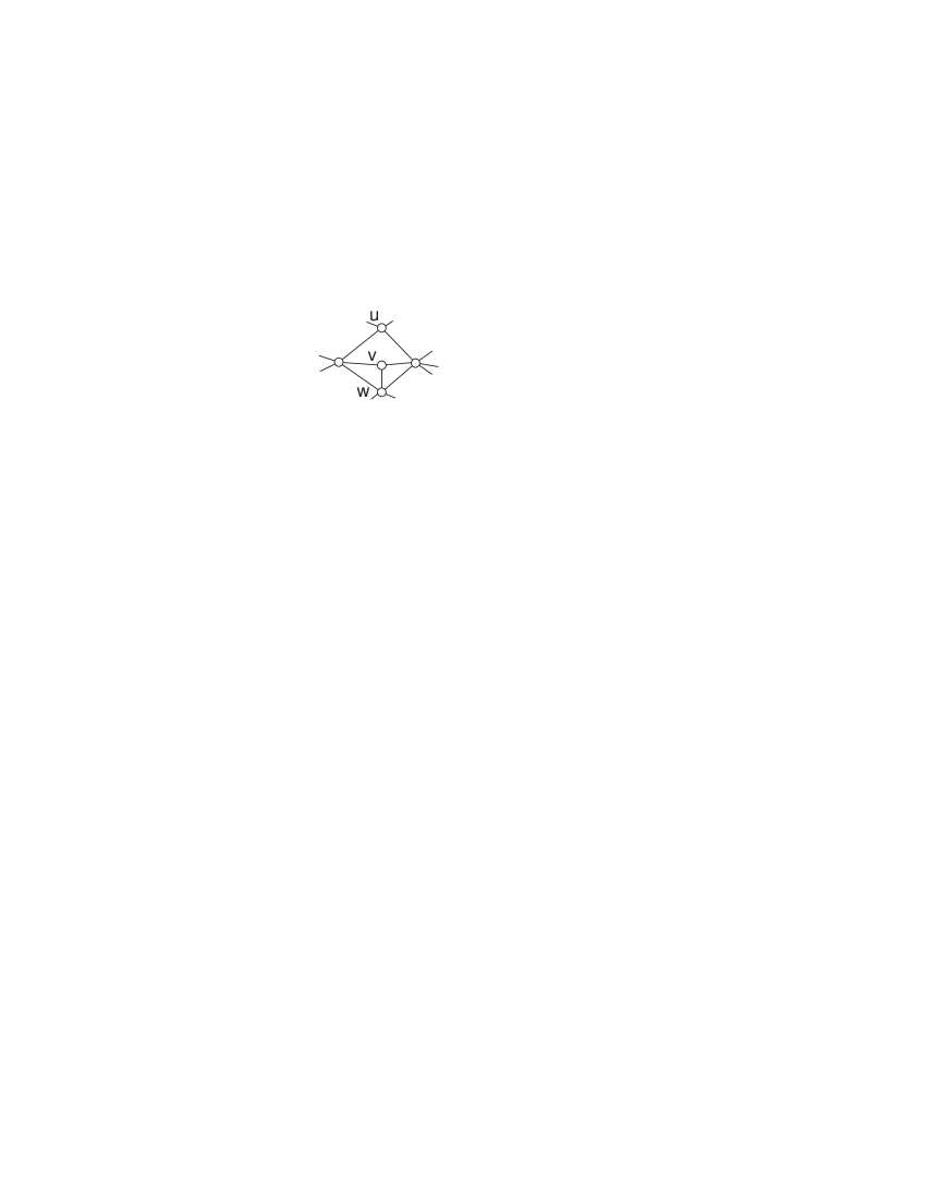
Figure 5: Example of ‘surround’ and ‘support’.

Examples Any vertex set is threatened by its neighbourhood, and by its neighbourhood minus a clique. A vertex of degree 2 is threatened by each of its neighbours, and supported by any vertex to which it has more than one 2-walk.

Theorem 7 enables supports and threats to be identified easily, especially single-vertex supports or threats. For a single vertex $b$, one way to identify the set $g(b)$ is to use the fact that it is the intersection of $\Gamma(b)$ with the set of vertices having $(d-1)$ 2-walks to $b$, where $d$ is the degree of vertex $b$. In fact one can avoid the need to calculate $g(b)$, because when the theorem applies, the edges from $b$ to $g(b)$ will all be dead by theorem 14, so $g(b)$ is an empty set after deletion of dead edges (defined below) and then the condition of theorem 7(ii) simplifies to $\Gamma(b)\subset\Gamma(a)$. This can easily be checked using an adjacency matrix or adjacency lists.

To discover threats to a single vertex, one can use 2-walks and the triangle number:

Theorem 8

For a given vertex $v$, let $x_{n}(v)=T(v)-(d-n)(d-n-1)/2$, where $T$ is the triangle number and $d$ the degree of $v$. $v$ is threatened by any set of $n$ of its neighbours having a total of $x_{n}(v)+m$ 2-walks to $v$, where $m$ is the number of edges between members of the set.

Corollary: A single neighbour having $(T(v)-(d-1)(d-2)/2)$ 2-walks to $v$ threatens $v$.

Proof: deletion of such a set $S$ would lower the degree of $v$ by $n$ and the triangle number by $x$. The new triangle number shows that $v$ is now only adjacent to a clique $K_{d-n}$. Therefore, using lemma 2(i), $(G-S)\ast v=(G-S)-v$ which is the condition defining a threat. $\Box$

Having gone to the trouble of identifying a threat or a support, the issue arises, will the property be preserved during further play, or must it be re-calculated for every new position?

Lemma 4

(i) If $A$ threatens $B$ in $G$ then $A$ threatens $(B\setminus\{b\})$ in $G-b$ and in $G\ast b$, $\forall b\notin A$.
(ii) If $A$ threatens $B$ in $G$ then $(A-a)$ threatens $B$ in $G-a$, $\forall a\in A$.
(iii) If $A$ supports $B$ in $G$ then $A$ supports $(B\setminus\{b\})$ in $G-b$ and in $G\ast b$, $\forall b\notin A$.
(iv) If $A$ supports $B$ in $G$ then $(A-a)$ supports $B$ in $G\ast a$, $\forall a\in A$.

Corollary For distinct sets $A,B_{1},B_{2}$, if $A$ threatens (supports) $B_{1}\cup B_{2}$ in $G$ then $A\cup B_{1}$ threatens (supports) $B_{2}$ in $G$.

Proof: (i),(iii) apply lemma 2(iii) to the set $B$ in the graphs $G-A$ and $G\ast A$. $\Box$ (ii) Note that $G-A\equiv(G-a)-(A-a)$ and apply it to both sides of $G-A\ast B=G-A-B$; the result follows immediately using commutation. $\Box$ (iv) use $G\ast A\equiv(G\ast a)\ast(A-a)$ and proceed as in (ii). $\Box$ The corollary can be obtained from (i) and it also follows immediately from lemma 2(iii) applied to the graph $G-A$ or $G\ast A$. $\Box$

Parts (i) and (iii) of the lemma show that a threat or a support can only be removed by playing directly on the threatening or supporting set. This is in contrast to domination, since if a vertex $v$ $P$-dominates a set $S$, a play by $\neg P$ on some other vertex in $S$ may remove the domination. In the context of computational analysis of a game the robustness is useful, because the computational effort invested in identifying a threat or support does not become valueless as soon as a new move is made. Parts (ii) and (iv) show that threat and support also survive play by one player in the threatening or supporting set. This again helps the computational problem, and is used in the proof of theorem 9. The corollary is used in theorem 10.

Next, observe that the action of ‘removing’ a threat by shorting the threatening set $A$ really transfers the threat to the neighbourhood of $A$:

$$G-A\ast B=G-A-B$$

$$\Rightarrow\;\;\;G-(\Gamma^{G}(A)\setminus B)\ast A\ast B=$$ (1)

$$G-(\Gamma^{G}(A)\setminus B)-A-B$$

where the superscript $G$ is to indicate that the neighbourhood in question is that in the original graph $G$, not the one obtained after shorting or deleting $A$ and $B$. In words the result is: if $A$ threatens $B$ then $\Gamma(A)\setminus B$ threatens $A\cup B$. To obtain the result, use the property of threat, that new edges introduced by shorting $B$ are all incident on $A$. Therefore shorting $B$ followed by cutting $(\Gamma^{G}(A)\setminus B)$ is equivalent to (results in the same graph as) cutting $B$ and $(\Gamma^{G}(A)\setminus B)$, i.e. cutting $\Gamma^{G}(A)$, and of course $\Gamma^{G}(A)$ threatens $A$.

This permits a straightforward proof of the following.

Lemma 5

A vertex of degree 3 that threatens each of two of its neighbours is in a set cut-dominated by the other neighbour.

Theorem 9

A vertex of degree 3 that threatens all its neighbours is in a lost set (and therefore so are its neighbours).

Proof. First we consider the lemma. Let $v$ be the vertex of degree 3, let $a,b$ be the threatened neighbours and let $w$ be the non-threatened neighbour. After shorting $v$, the threat that it offered to $a$ and $b$ is transferred as in eq. (1), such that $a$ is now threatened by the set $\{b,w\}$ and $b$ is threatened by the set $\{a,w\}$. After cutting $w$, the resulting situation is one in which each of the remaining vertices threatens the other (lemma 4(ii)), so both are lost (corollary to theorem 6). It follows that $w$ cut-dominates $\{v,a,b,w\}$.

To prove the theorem, we show that Cut has a second player winning strategy for ${\cal M}_{G,S}$ where $S=\{v,a,b,w\}$, as follows. If Short does not short $v$, then Cut deletes it and wins (since it threatens all the others, the graph is now $G-S$). Otherwise, after shorting $v$, Cut may delete any vertex and thus leave a mutually threatening pair, hence a lost pair. $\Box$

Note that theorem 9 allows the reduction of a 4-vertex subgraph that is not reducible by theorem 2 alone.

There is no partner result to eq. (1) following the removal of a support. In this case there does not necessarily remain any supporting set of vertices (one may easily show that a vertex has no supporting set if and only if it is an articulation vertex (cut-vertex) of the graph). When there is no single supporting vertex, but a larger supporting set exists, there is no simple rule for finding a small or minimal such set.

Some further captured or lost sub-graphs not reducible by theorem 2 are covered by the following theorem.

Theorem 10

For any set of $P$-dominated vertex pairs $\{a_{i},b_{i}\}$, let $A$ be the set of dominating vertices and $B$ the set of dominated vertices (i.e. $A=\Cup_{i}\{a_{i}\}$, $B=\Cup_{i}\{b_{i}\}$ where $a_{i}$ $P$-dominates $\{a_{i},b_{i}\}$). If for such a set of pairs, the pairs are cut-dominated and $B$ threatens $A$, then $A\cup B$ is lost; if the pairs are short-dominated and $B$ supports $A$, then $A\cup B$ is captured.

Proof: For brevity we only present the proof for $P$=Cut; the proof for $P$=Short is similar. The 2nd-player winning strategy for Cut is as follows. Each move by Short must be on one of the pairs $a_{i},b_{i}$; Cut replies by cutting the other vertex of the pair. Let $G_{n}$ be the reduced graph at the $n$’th pair of moves. On each occasion that a vertex in $A$ is shorted, the graph develops to $G_{n+1}=G_{n}\ast a_{i}-b_{i}$. On each occasion that a vertex in $B$ is shorted, the graph develops to $G_{n+1}=G_{n}-a_{i}\ast b_{i}=G_{n}-a_{i}-b_{i}$ by the definition of threat (see theorem 6). Hence after all vertices are coloured, the reduced graph is the same as one in which all of $B$ is cut. Let $A_{1}\subset A$ be the part (possibly empty) of $A$ that was shorted, then obviously $A_{0}\equiv A\setminus A_{1}$ was cut, so the final reduced graph is $G\ast A_{1}-A_{0}-B$. By the corollary to lemma 4, $B\cup A_{0}$ threatens $A_{1}$, therefore this reduced graph is equal to $G-A-B$, therefore the multi-Shannon game is won by Cut. $\Box$ An example is shown in figure 6.

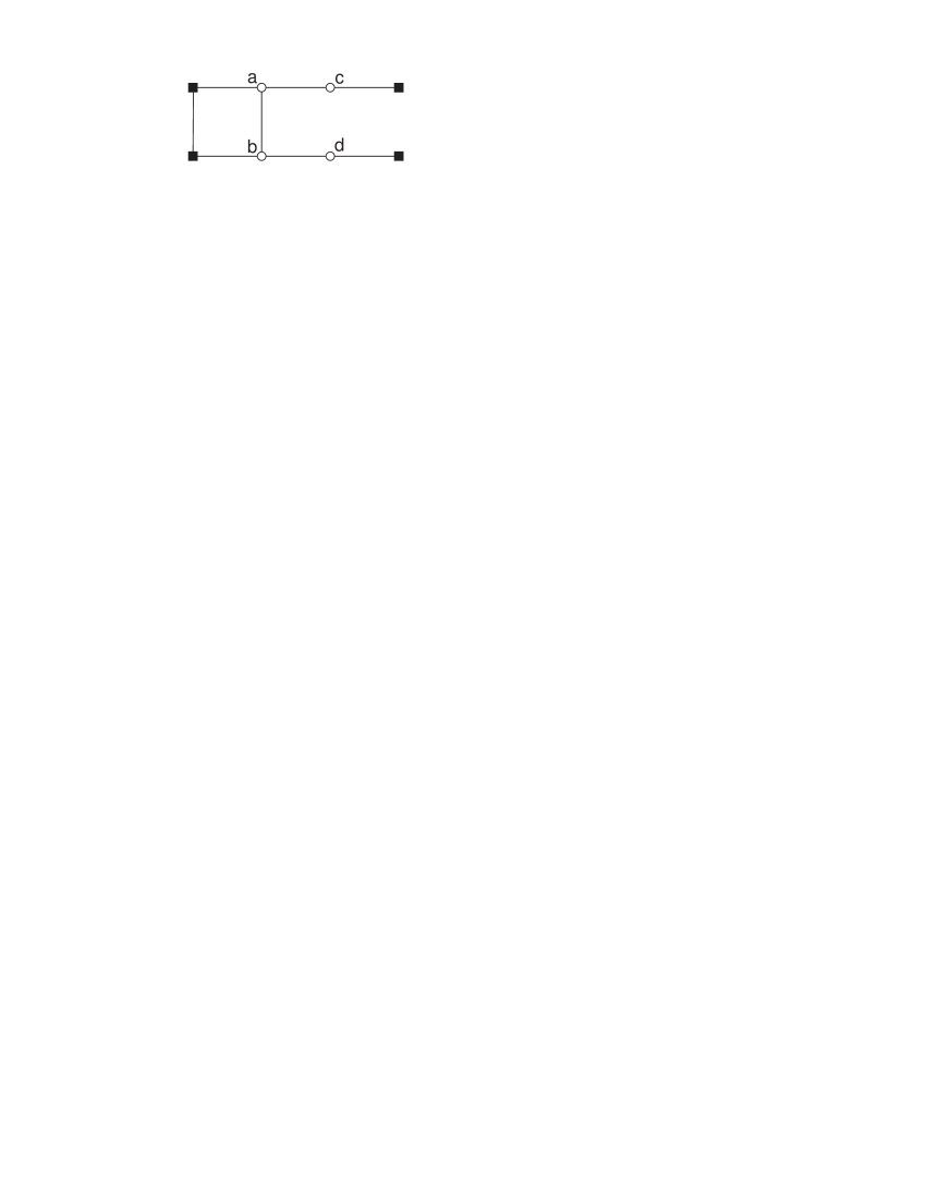
Figure 6: Example multi-Shannon game that is not reducible by mutually dominating pairs, but can be solved by pair-sets (theorem 10). In the game shown, $a$ threatens $c$ and $b$ threatens $d$ and $\{c,d\}$ threatens $\{a,b\}$ hence there is second-player winning strategy for Cut, by theorem 10, so the set $\{a,b,c,d\}$ is lost.

Finally, we note a Cut-winning condition for the Shannon game that is easy to check if threats are in any case being examined. (Simple 2nd-player Short-winning conditions are well known, such as the presence of more than one 2-walk between terminals. By considering the block graph one can derive further conditions for a Cut win, but to check this is relatively costly in computational terms.)

Theorem 11

In the Shannon game, if the neighbours of a terminal $t$ are all threatened by distinct vertices, then Cut has a 2nd-player winning strategy. The strategy is: if Short shorts a vertex in $\Gamma(t)$, then cut the corresponding threat vertex; if Short shorts a vertex threatening $v\in\Gamma(t)$, then cut $v$, otherwise cut any remaining vertex in $\Gamma(t)$.

Corollary If all the neighbours of a terminal except one are threatened by distinct vertices, then Cut has a 1st-player winning strategy, namely to cut the non-threatened neighbour.

Example If a terminal $t$ has neighbours all of degree 2, and no vertex has more than one 2-walk to $t$, then Cut is the winner.

4.1 Discussion

The theorems concerning threat and support simplify the analysis of the Shannon game, and the computational task of identifying lost or captured sets.

We described the multi-Shannon game in section 3 because this is the right way to understand capture and loss in general. However, we don’t need that concept to understand support and threat. If we ignore the multi-Shannon game we can still prove the essential property of threat pairs and supporting pairs, namely that $W(G,x)=W(G\ast a\ast b,x)$ if $a$ and $b$ support each another, and $W(G,x)=W(G-a-b,x)$ if $a$ and $b$ threaten each other (for single vertices $a$, $b$). For, if $a$ and $b$ support each other then $G-a\ast b=G\ast a-b=G\ast a\ast b$. Therefore if $W(G,x)=$Cut (for some value, not necessarily all values, of $x$) then there is a winning strategy whose cutset does not require $a$ or $b$, hence they are spectators. If the winning cutset did require one of $a$ or $b$, then at some stage Cut must cut it, but then Short can reply such that the position is equivalent, in the colouring model, to one in which both are coloured black (Short’s colour) and we have a contradiction. If $W(G,x)=$Short then obviously $W(G\ast a\ast b,x)=$Short since shorting vertices as a “free move” can never be disadvantageous to Short (this is obvious in the graph colouring model). The same argument with appropriate adjustments proves the corresponding result for a threat pair. $\Box$

The graph properties identified in theorems 7 and 8 suffice to discover (through the above argument, or by using theorems 6, 2) all the examples of lost pairs presented in [2] (they are called ‘cut-captured’ there), and all the examples of captured pairs presented in [2], without the need for any further pattern search. An illustrative example is shown in figure 7.

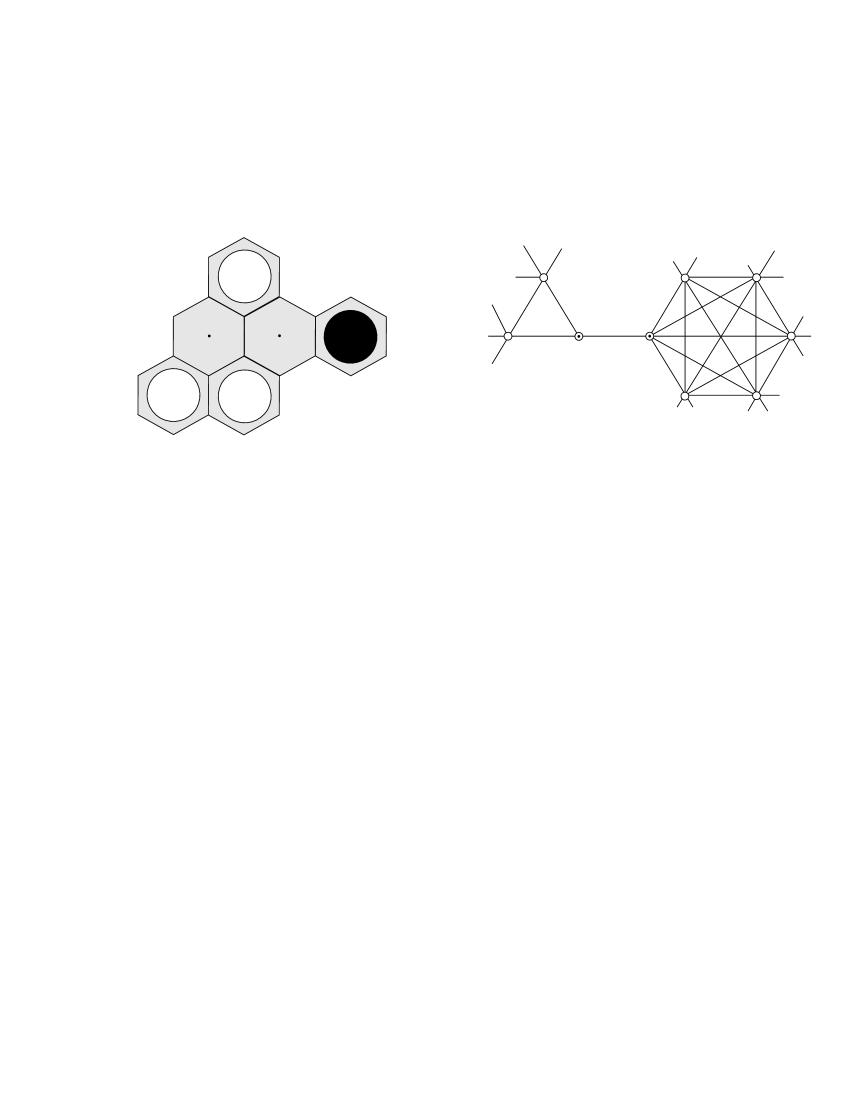
Figure 7: Example of a threat-pair arising in Hex. The left diagram shows part of a Hex board, with Short playing black. The right diagram shows the equivalent graph, supposing the cells not shown on the left are empty. Theorem 8 can be used to show that the dotted cells (vertices) threaten each other. If the surrounding cells are not empty, the effect on the reduced graph is merely to grow or shrink the cliques, see lemma 4.

Björnsson et al. also presented some examples of won multi-Shannon games that arise in Hex but are not reducible by mutually dominating pairs. All of these are covered by theorems 7, 9 and 10. Figures 8 and 9 present two examples. These arise from two dual graphs representing the same hex position; figure 8 is a Cut-win; figure 9 is a Short-win. The captions give the proofs.

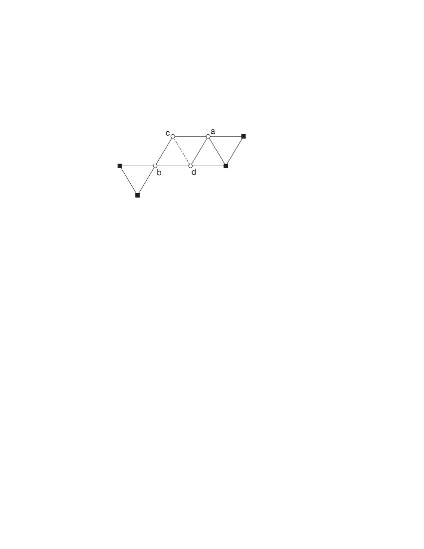
Figure 8: Example multi-Shannon game that can arise in Hex, and that can be solved by pair-sets (theorem 10). First note that $a$ threatens $c$, and observe from theorem 14 that the edge $cd$ is dead. After deleting it, $b$ threatens $d$. Also, $\{c,d\}$ threatens $\{a,b\}$ (since $\Gamma(a)\setminus\{c,d\}$ is a clique and $\Gamma(b)\setminus\{c,d\}$ is a clique, lemma 3 and theorem 7). Therefore the set of pairs $\{\{a,c\},\{b,d\}\}$ realise the condition of theorem 10 and therefore $\{a,b,c,d\}$ is lost.

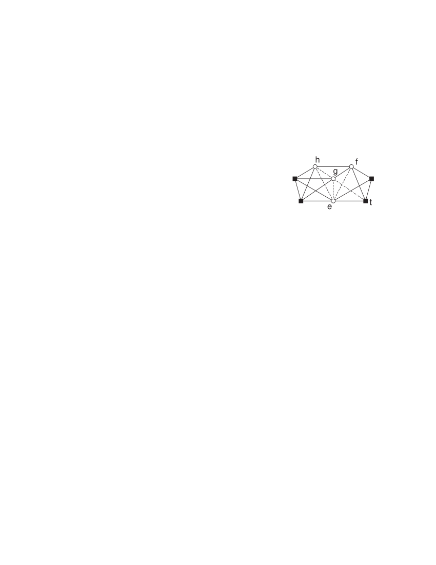
Figure 9: A multi-Shannon game that can arise in Hex and that is not reducible by mutually dominating pairs, but can be solved by using and-, or-rules for multiple connections, see appendix, or by using supporting sets. There is a second-player winning strategy for Short, hence vertices $\{e,f,g,h\}$ are ‘captured’. Proof: $e$ supports each of $f$, $g$, $h$ (theorem 7) so each of them is locally losing for Cut. $f$ short-dominates $\{f,g,h\}$ since after shorting $f$, $g$ and $h$ support each other and are therefore captured (theorems 6, 2). Also, $\{f,g,h\}$ supports $e$. Therefore we have that Short dominates a set that supports $e$, hence $e$ is locally losing for Cut. Thus all moves are locally losing for Cut, therefore Short has a second player winning strategy. (The edges shown dashed are dead, and this can be discovered using theorem 14, but we didn’t need to invoke that here. The edge $gt$ (shown dash-dotted) is not dead but it is a spectator. If its spectator status could be discovered conveniently (without first solving the game) then it could be deleted, and then the game could be reduced using support pairs.)

In a computational setting, one can track both threat and support by maintaining a (representation of a) directed graph for each. This allows threats and supports to be detected incrementally and locally as the game proceeds (at any moment during the course of a game, one only has to examine the neighbourhood of the part of the graph which just changed). Theorems 7 and 8 enable threats and supports to be detected rapidly. Once detected they are stable (lemma 4). Suppose for example that at some stage it is found that $a$ threatens $b$. Such a threat remains until such time as $a$ is shorted, so it does not need to be reconsidered as the game proceeds. Thereafter neither player should play at $b$, until such time as $a$ is shorted. This is because if Cut wants to delete $b$, he may as well delete $a$ and then $b$ dies, and Short can be sure that a play at $b$ is useless to him, since Cut could, if he chose, reply at $a$ which would return a position equivalent to the one Short was considering, but with two vertices deleted.

If subsequently a position develops in which $b$ also threatens $a$, then both can be deleted immediately. Similar considerations apply to a supported vertex, with the roles reversed.

5 Dead edges and vertices

If $W(G-v,x)=W(G\ast v,x)\forall x$ then we say vertex $v$ is a spectator: no matter who is to play, the game outcome is not influenced by deleting or shorting $v$.

A stronger property is discussed in [2]. In the graph colouring model, suppose at a given game position we colour all the remaining uncoloured vertices in some arbitrary black and white pattern, without respect to taking turns. Such a complete colouring $c$ produces some final position ${\cal G}_{c}$ with a definite winner.

Definition In a given graph $(G,\{t_{1},t_{2}\})$ a non-terminal vertex $v$ is dead if, for every complete colouring ${\cal G}_{c}$ obtainable from $G$, the winner of ${\cal G}_{c}$ is independent of the colour of $v$.

Definition In a given graph $(G=(V,E),\{t_{1},t_{2}\})$ an edge $e\in E$ is dead if, for every complete colouring ${\cal G}_{c}$ obtainable from $G$, the winner of ${\cal G}_{c}$ does not change if $e$ is deleted. An edge $e\notin E$ is dead if it is dead in $(G+e,\{t_{1},t_{2}\})$.

The dead vertex idea was discussed in [2]; here we extend the concept to a dead edge. This will allow us to introduce some new useful results.

Theorem 12

A vertex is dead if and only if all edges incident on it (and present in the graph) are dead.

Proof: Consider the final position after some complete colouring obtainable from the given initial position. ($\Leftarrow$) If all the edges incident on $v$ are dead, then we can delete them without changing the winner, and then $v$ is isolated so it is obvious that its colour does not influence any outcome. ($\Rightarrow$) If the vertex is dead, then if the winner is Short the vertex is not needed so its edges are irrelevant, and if the winner is Cut it is still Cut if any edge is deleted. In either case the outcome is unchanged if any of the incident edges are deleted. $\Box$

Corollary Adding or deleting dead edges in a game $G$ does not influence whether or not any vertex is dead in $G$.

Proof: If a vertex is dead, then after adding or deleting dead edges it still satisfies the the sufficient condition of the theorem. If a vertex is not dead, then adding or deleting dead edges does change the fact that it has a non-dead edge so does not satisfy the necessary condition of the theorem.

In a given game position, the set of dead vertices can include some that are already coloured by one or other player (but changing their colour will not affect the outcome). If a vertex is dead then it is a spectator.

Dead vertices are in general hard to identify: recognising dead vertices in the Shannon game is NP-complete [2]. In this section we present some theorems that allow some dead vertices and dead edges to be identified easily, using readily calculated properties of the graph. The first case, a subgraph with a clique cutset (theorem 13), is already known, see for example [1], it is included here for completeness and because the proof is instructive.

Theorem 13

A terminal-free subgraph with a clique cutset is dead (i.e. all its edges and vertices are dead).

Proof: The vertices of the subgraph are a subset of some vertex set $V$ whose neighbourhood is a clique. For such a set $G\ast V=G-V$. We will prove that all the members of $V$ are dead. Pick a vertex $v\in V$. First consider some complete colouring $\cal C$ in which $v$ is black (Short’s colour). Then, if the winner is Cut it is obviously still Cut if $v$ is changed to white. If the winner is Short then it is still Short if all the rest of $V$ is coloured black (since adding edges cannot be bad for Short). Since the reduced graph $G\ast V$ is the same as $G-V$, the winner must still be Short if all of $V$ is white. Adding edges to the reduced graph $G-V$ cannot be bad for Short, so the winner remains Short if we return to the colouring $\cal C$ with just the colour of $v$ changed from black to white. This completes the proof for complete colourings in which $v$ is black. A similar argument, adjusted appropriately, applies for complete colourings in which $v$ is white. $\Box$

Example Non-terminal simplicial vertices are dead. (For example, pendant vertices are simplicial.)

Clique cutsets can be discovered by an $O(n^{3})$ algorithm due to Whitesides [9, 10]. There can be dead vertices which do not satisfy the condition of theorem 13; figure 10(b) shows an example of a dead vertex where $G\ast v\neq G-v$ (see theorem 16).

Figure 10: Examples of dead vertices. A vertex shown with a dot is dead. A filled square vertex is a terminal in a Shannon game. (a) illustrates theorem 13; (b) illustrates theorem 16 and is an example where $G\ast v\neq G-v$.

Definition An edge between a vertex $v$ and a surrounding vertex (i.e. one surrounding a set containing $v$) is called transverse.

Theorem 14

If $w$ surrounds a terminal-free subgraph containing $v$, then $vw$ is dead. More succinctly, transverse edges to a terminal-free subgraph are dead.

Corollary I If $w$ surrounds non-terminal $v$ then $vw$ is dead. (This condition is equivalent to

$$A^{2}(v,w)=d(v)-A(v,w)$$

where $A$ is the adjacency matrix and $d$ is degree.)

Corollary II If $\Gamma[v]$ is terminal-free and

$$A^{3}(v,w)=\sum_{i\neq w}A^{2}(v,i).$$ (2)

then all edges between $w$ and $\Gamma[v]$ are dead.

The theorem is based on the idea that if a winning path passing from $w$ to $v$ must continue to a neighbour of $w$ before it can reach a terminal, then the part through $v$ must be irrelevant. (This is loosely reminiscent of, but clearly different from, lemma 1 of Hendersen et al. [11]). The corollaries give two examples of the condition of the theorem that are easy to identify in practice. An example of corollary I is shown in figure 2, where vertex $c$ surrounds vertex $a$. In corollary II, all walks from $v$ either remain in $\Gamma[v]$ or pass through $\Gamma[w]$; figure 11 shows an example.

Proof: invoke the graph-colouring model, and let $e=vw$ be the edge. For each complete colouring invoked in the definition of dead edges, the final position is either won or lost for Short. If it is lost then obviously the deletion of $e$ will not change the win-value. If it is won then $e$ is only alive if the existence of a winning path requires it. However, for every short-winning path $\left<\ldots,w,v,P,a,\ldots\right>$ containing $e$, where $P$ is a sub-path (possibly empty), there is a winning sub-path not containing $e$: $\left<\ldots,w,a,\ldots\right>$ (as long as neither $v$ nor the vertices of $P$ are terminal). $P$ refers to that part of the path after $v$ which remains on the subgraph surrounded by $w$. Eventually the winning path must emerge from this vertex set, and when it does the next vertex $a$ is a neighbour of $w$, by the condition of the theorem. $\Box$

Proof of eqn (2). Corollary II presents a sufficient but not necessary condition that $w$ surrounds $\Gamma[v]$. Consider all $2-$walks from $v$. Let $N_{1}$, $N_{2}$, $N_{3}$ be the number that end on a neighbour of $w$, on $w$ itself, and on neither, respectively. Then (since the $i$’th power of the adjacency matrix gives the number of $i$-walks),

$$\sum_{i}A^{2}(v,i)=N_{1}+N_{2}+N_{3}$$

and

$$A^{3}(v,w)=N_{1},\;\;\;\;\;A^{2}(v,w)=N_{2}.$$

If $N_{3}=0$ then $w$ surrounds $\Gamma[v]$, since then all walks from $v$ of length 2 or more start with a part that passes through $\Gamma[w]$. (This is a sufficient but not necessary condition; it ignores the possibility that there may be a triangle including $v$ and a non-neighbour of $w$, and also the possibility of two-walks from $v$ that pass through $\Gamma(w)$ to a vertex other than $w$). Substituting $N_{3}=0$ into the above set of equations gives (2).

The discovery of even a single dead edge can considerably simplify analysis of a given Shannon game. For example, figure 11 shows a case where after deleting one dead edge, three vertices can also be eliminated because it becomes obvious that they form a lost set. In the context of a larger game, this in turn reduces the amount of further information needed to be handled by a solution algorithm, such as the set of vertex sets forming weak and strong ‘links’ or ‘virtual connections’ [1].

Figure 11: Edge $vw$ is dead (by corollary II to theorem 14); after deleting it, one may discover by theorem 2 (threat pairs) that the pairs $\{a,v\}$ and $\{v,b\}$ are lost.

We conclude this section with two theorems which stem from the special role played by terminals in the Shannon game.

Theorem 15

An edge between neighbours of a given terminal is dead.

Proof: An edge $uv$ is only alive if the existence of a Short-coloured path between the terminals requires it in some complete colouring. Let $t$ be the terminal mentioned in the theorem. All paths sought by Short start or end on $t$. In the condition of the theorem, both $u$ and $v$ are in $\Gamma(t)$, and therefore any path $\left<t,\ldots u,v,\ldots\right>$ has a subpath $\left<t,v,\ldots\right>$, and any path $\left<t,\ldots v,u,\ldots\right>$ has a subpath $\left<t,u,\ldots\right>$, therefore edge $uv$ is not required by Short in order to form any path to or from $t$. Therefore $uv$ is not required by Short in any complete colouring, so is dead. $\Box$

Theorem 16

A terminal-free vertex set surrounded by a terminal is dead.

(Figure 10b shows an example.) We offer two proofs. Proof 1: The closed or open neighbourhood of the terminal can be converted into a clique by adding edges that are dead by theorem 15. After this is done the vertex set in question has a clique cutset so is dead by theorem 13, and therefore it is dead in the original graph by the corollary to theorem 12. $\Box$

Proof 2: Let $U$ be the vertex set in question. For a vertex to be alive, it is necessary that a path sought by Short requires it in some complete colouring. However, all paths sought by Short start or finish on $t$, and in the conditions of the theorem, any path $\left<t,\ldots P,a,\ldots\right>$, where $P$ is on $U$, has a subpath $\left<t,a,\ldots\right>$, since any non-$t$ neighbour of $U$ is a neighbour of $t$. Therefore the vertices of $U$ are dead. $\Box$

6 Statistics on small graphs

The usefulness or otherwise of the theorems presented in this paper, for the purpose of analyzing the Shannon game, can be roughly assessed by exploring how often the conditions of the various theorems arise in Shannon games in general. To this end, we examined all graphs on up to 10 vertices, and counted those in which the conditions of various of the theorems arise. Table 1 shows the results. The main thing to notice is that the numbers in columns 3–6 of the table are small compared to the number of connected graphs (column 2). This shows that the great majority of graphs satisfy one or more of the conditions, so the theorems will be useful in practice to simplify most games.

size	graphs	S-free	$\perp$-free	$\geq 2\,\triangle$-free	4 & 5
1	1	0	1	0	0
2	1	0	0	1	0
3	2	0	0	1	0
4	6	1	1	3	1
5	21	4	2	10	2
6	112	24	9	52	7
7	853	191	46	363	34
8	11117	3094	507	4022	327
9	261080	95204	11800	72594	5897
10	11716571	5561965	626586	2276219	213064

Table 1: Numbers of graphs with various properties. In all cases only connected graphs are counted. The second column shows the total number of connected graphs on the given number of vertices. ‘S-free’ means simplicial-free (i.e. no simplicial vertices). ‘$\perp$-free’ means there are no transverse edges (i.e. those which are dead by corollary I to theorem 14 if the surrounded vertex is non-terminal). The 5th column counts graphs containing at least 2 triangle-free vertices—only Shannon games on such graphs are free of edges that are dead by theorem 15. The last column counts graphs satisfying conditions of both columns 4 and 5.

7 Conclusion

The new ideas presented in this paper are of three kinds. We presented new methods to identify dead edges and dead vertices: theorems 14, 15, 16. Secondly, we presented methods to solve some multi-Shannon games (theorems 9, 10) that are not easily reducible. Thirdly, we introduced the idea of ‘threat’ and ‘support’ (in our terminology). These are in general stronger conditions than ‘domination’ in the terminology of [2]. This makes them rarer but easier to identify. In the case of a two-vertex set, threat or support is equivalent to domination (theorem 6). Therefore to identify mutually dominating pairs (which are consequently either lost or captured) it is sufficient to identify mutually threatening or supporting pairs, and we have presented, in theorem 8 and corollary I to theorem 14, easily-computed properties that can be used to identify threats and supports without the need for pattern-searching algorithms.

This work was supported by Oxford University.

Appendix: or and and rules

Definition A strong multi-link is a set of vertices $V$ and terminals $T$ such that with play restricted to $V$, Short can guarantee to cause $T$ to become a clique (in the reduced graph) if he plays first or second. A weak multi-link is a set of vertices $V$ and terminals $T$ such that with play restricted to $V$, Short can guarantee to cause $T$ to become a clique if he plays first, but not if he plays second. A pivot of a weak multi-link is any vertex which, if shorted, makes the link become strong.

In either case the vertex set $V$ is said to be the carrier of the multi-link. The definition of a strong multi-link includes the case where the carrier is the empty set and the terminals are already a clique. Usually the terminals $T$ are a subset of $\Gamma(V)$, but they do not need to be the whole of $\Gamma(V)$ so the existence of a strong multi-link $V,T$ does not necessarily imply that $V$ is captured.

We can now state the generalized or-rule:

Theorem 17

(‘or-rule’): If a set of weak multi-links between given terminals has zero total intersection, then the union of the weak multi-links is a strong multi-link between the terminals.

Proof: obvious, and can be compared with that of theorem 5.

The ‘and-rule’ can be generalized in more than one way. The simplest is, arguably:

Theorem 18

(‘and-rule’) If two strong multi-links $V_{1},T_{1}$ and $V_{2},T_{2}$ have intersecting terminals and non-intersecting carriers, then the combination $V_{1}\cup V_{2},T_{1}\oplus T_{2}$ is a weak multi-link, pivoted by any vertex in $T_{1}\cap T_{2}$.

Proof: use commutation and suppose the opening Short move is performed last. The first strong multi-link guarantees that Short can cause $T_{1}$ to become a clique, the second guarantees that Short can cause $T_{2}$ to become a clique. When a vertex in $T_{1}\cap T_{2}$ is then shorted, $T_{1}\oplus T_{2}$ becomes a clique.

As an example, we apply these rules to the multi-Shannon game shown in figure 9. $h$ is the carrier of a weak multi-link from the left terminals to $f$; $g$ is the carrier of another such weak multi-link, therefore by the or-rule, $\{h,g\}$ is the carrier of a strong multi-link between the left terminals and $f$. $f$ being adjacent to both right terminals, there is a strong multi-link from $f$ to the right terminals with empty carrier, and therefore by the and-rule $\{h,g,f\}$ is the carrier of a weak multi-link between all the terminals, pivoted by $f$. Finally, $e$ is the carrier of another weak multi-link between all the terminals, so using the or-rule a second time, $\{h,g,f,e\}$ is the carrier of a strong multi-link between all the terminals of the multi-Shannon game, so the game is won by Short.

References

- [1] R. Hayward and J. van Rijswijck. Hex and combinatorics. Discrete Math, 306:2515–2528, 2006. (formerly Notes on Hex).
- [2] Y. Björnsson, R. Hayward, M. Johanson, and J. van Rijswijck. Dead cell analysis in hex and the shannon game. In Graph Theory in Paris: Proc. of a Conference in Memory of Claude Berge (GT04 Paris), pages 45–60. Birkauser, 2007.
- [3] A. Lehman. A solution of the shannon switch game. J. Soc. Indust. Appl. Math., 12:687–725, 1964.
- [4] A. Beck, M. N. Bleicher, and D. W. Crowe. Excursions into Mathematics. Worth, New York, 1969. Millennium Edition (A.K. Peters, New York 2000).
- [5] D. Gale. The game of hex and the Brouwer fixed point theorem. American Mathematical Monthly, 86:818–827, 1979.
- [6] S. Reisch. Hex ist pspace-vollständig. Acta. Informatica, 15:167–191, 1981.
- [7] V. V. Anshelevich. An automatic theorem proving approach to game programming. In Proceedings of the Seventh National Confernce of Artificial Intelligence, Menlo Park, California. Birkauser, 2000.
- [8] V. V. Anshelevich. A hierarchical approach to computer hex. Artificial Intelligence, 134:101–120, 2002.
- [9] Sue Whitesides. An algorithm for finding clique cut-sets. Inf. Process. Lett., 12:31–32, 1981.
- [10] Fǎnicǎ Gavril. Algorithms on clique separable graphs. Discrete Mathematics, 19:159–165, 1977.
- [11] Philip Henderson, Broderick Arneson, and Ryan B. Hayward. Solving hex. In Proceedings of the 21st international jont conference on Artifical intelligence, IJCAI’09, pages 505–510, San Francisco, CA, USA, 2009. Morgan Kaufmann Publishers Inc.