A NEW APPROACH TO LINAC RESONANCES AND EQUIPARTITION ?

Abstract

In this note we refer to a recent paper “Equipartition, Reality or Swindle?” [1] presented by Lagniel at HB2012, Beijing, which claims to challenge the currently used approach to describe space charge resonances and emittance exchange with the help of linac-specific stability charts. On the one hand we agree with the general observation that enforcing equipartition (EP) would be an unnecessary constraint; however, we find that the heuristic single-particle arguments and examples presented by Lagniel are speculative and cannot be reconciled with results from self-consistent computer simulation. Thus, we see no justification for Lagniel’s suggestions, which include a modified EP definition (treating $x$ and $y$ as correlated). Instead, we suggest to maintain the current approach and to continue using the “conventional” EP definition. With our findings we also respond in some detail to Lagniel’s “Topics of Discussion”.

1 Introduction

One of the widely accepted criteria in high-current linac design is to use linac-specific stability charts to identify parameter regions, where emittance exchange between the longitudinal and transverse degrees of freedom might occur. It is common understanding that this exchange is caused by space charge resonances. Plotting the rms tune ratios and tune depressions from simulation codes on these stability charts is a widely used approach in new linac projects in order to deal with the problem of undesirable emittance exchange. These charts include the physics of phase space flow on a perturbational level, and under the effect of coupling between two degrees of freedom due to space charge “pseudo-multipoles” [2]. The resulting resonance stop-bands proliferate not only the location of possible resonances lines (as ring resonance diagrams normally do), they also represent their space charge dependent driving terms. Obviously, particle-in-cell (PIC) simulation is necessary to examine the validity of the charts, which was carried out successfully under a great variety of conditions (for a recent discussion including relevant references see Ref. [3]).

Lagniel’s paper is based on three arguments mainly:

(1) The law of EP in a rigorous sense holds only for ergodic systems (undeniable - see our comments in the before last section).

(2) If used at all, the “conventional” EP condition employing an rms energy ratio $T$ as shown in Eq. 1

$$T\equiv\frac{\epsilon_{z}k_{z}}{\epsilon_{x}k_{x}}=1,$$ (1)

(all quantities understood as rms quantities) “is wrong” and should have a factor 2 in the denominator, with the argument that the sum of transverse energies should be in balance with the longitudinal energy (see Eq. (5) in Ref. [1]).

(3) The conventional EP-condition does not prevent resonant emittance exchange.

Below we examine first assertion (3) in the next section, followed by a critical discussion of (2), and concluding with comments on Lagniel’s “Topics of discussion” as well as some final remarks.

2 PIC examination of Lagniel’s examples

In the following we undertake a careful examination of the two examples of equipartitioned and non-equipartitioned beams by using the TRACEWIN particle-in-cell simulation of realistic bunched beams in a periodic FODO lattice, with no acceleration and RF gaps to keep the bunches longitudinally. We employ 100.000 simulation particles and an input distribution following the TRACEWIN standard option of randomly generated particles in the 4d transverse hyper space as well as randomly in the longitudinal phase plane ellipse.

The parameters of the exactly equipartitioned example ($T=1$ by the conventional definition of Eq. 1) described in Eqs. (6)-(9) of Ref. [1] are identically chosen as $\epsilon_{z}/\epsilon_{x}=1.18$, $k_{z}/k_{x}=0.85$ , $k_{x}/k_{0x}=0.75$ and $k_{0z}=73^{o}$ (per cell). The beam is matched - as much as possible with TRACEWIN - and then propagated over 100 cells (45 m). The result is shown in Fig. 1 including the tune footprint from TRACEWIN on the stability chart for $\epsilon_{z}/\epsilon_{x}=1.18$. Note that the vertical line at $k_{z}/k_{x}=1$ (the “main” or “fourth order” resonance $2k_{z}-2k_{x}=0$) in the stability charts corresponds to the diagonal in Lagniel’s Figure1.

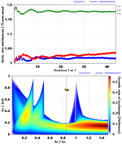
Figure 1: Evolution of rms emittances for example on the EP condition, with stability chart for $\epsilon_{z}/\epsilon_{x}=1.18$ (dotted line is EP condition $T=1$).

It is noted that there is a 2-3% initial transverse emittance growth, whereas the longitudinal emittance is only oscillating around its initial value (1.18). Running this case over twice the distance we find that $\epsilon_{z}$ still remains constant within $\pm 0.1\%$ and $\epsilon_{x},\epsilon_{y}$ grow slowly, but $<1\%$. Hence, we find absence of emittance exchange - consistent with the “safe” distance of the tune footprint from the stop-band in the stability chart. Note here that the width of the stop-band of the main resonance (near $k_{z}/k_{x}=1$) is shrinking to zero for $\epsilon_{z}/\epsilon_{x}\rightarrow 1$ (see Ref. [3]).

Thus, contrary to Ref. [1], we find that the proximity of the EP working point to the main resonance $k_{z}/k_{x}=1$ is not adversary to the stability of the rms emittances. In fact, Lagniel is drawing his conclusions from a schematic picture of a tune footprint in his Figure 1, which he finds indicative of an overlap with the resonance $k_{z}/k_{x}=1$. Firstly, the square box tune footprint is un-physical - particles not seeing any space charge in one direction (as the ones on the two sides adjacent to the right upper corner, which is given by the zero-current tunes) don’t exist. Consistent tune footprints in a $k_{z}-k_{x}$ plane are actually necktie-shaped rather than square-boxed, which reduces the overlap. Secondly, it is necessary to consider the response of the bunch as a whole, i.e. the property of the ensemble versus that of single particles. Individual particles may have growing amplitudes in one direction, which can be compensated by other particles with shrinking amplitudes, and no net effect.

Not surprisingly there is a fast ($<20$ cells) and pronounced emittance exchange of about 10% , if we lower the transverse focusing such that $k_{z}/k_{x}=1.02$ and the working point sits exactly on the stop-band, while the beam is initially weakly non-equipartitioned with $T=1.2$ (Fig. 2).

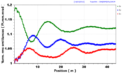
Figure 2: Same as Fig. 1, but $k_{z}/k_{x}=1.02$.

As far as the second example, following Eq. (10) of Ref. [1] (with $k_{0x}$ further lowered to 50^o), we agree, in principle, that no emittance exchange should be expected. The distance to the fourth order resonance line $k_{z}/k_{x}=1$ is large enough, equally to the third order line $k_{z}/k_{x}=2$ (i.e. $k_{z}-2k_{x}=0$). It should be noted, however, that the driving term for this third order mode requires a sextupolar component in the space charge potential. Such a third order term is absent in the matched initial beam, where only even powers in the space charge potential exist. Therefore we cannot see how it enters into Lagniel’s frame of discussion, if the driving term is absent. In PIC simulation however, equally in our stability chart, this driving term evolves self-consistently from a resonant unstable behaviour of the third order mode building up from initial noise. An example for the effect of this third order mode on the extended stability chart including $k_{z}/k_{x}=2$ is given below in Fig. 4.

3 Do we need a new EP-formula?

In the discussion preceding his Eq. (5), Lagniel argues that the conventional EP condition Eq. 1 “is wrong” and should have a factor 2 in the denominator to account for “a total correlation between the two radial degrees of freedom”. We cannot follow this argument, because dynamically speaking each degree of freedom is independent - no matter what its initial tune and emittance values are. But let us use simulation to help decide between the conventional EP condition and Lagniel’s proposition. To this end let us call Lagniel’s modified energy ratio $T^{*}$ ($=T/2$ and the condition $T^{*}=1$ the modified equipartition condition EP^∗.

Let us start with Case 1: fulfilling the “conventional” EP condition ($T=1$, but $T^{*}=1/2$), with $\epsilon_{z}/\epsilon_{x}=1$, $k_{z}/k_{x}=1$ (also $k_{0z}/k_{0x}=1$) and $k_{0z}=73^{o}$ per cell as well as a transverse tune depression of $k_{x}/k_{0x}=0.72$. The resulting rms emittances as well as the footprint of tunes on the stability chart are shown in Fig. 3.

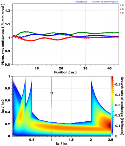
Figure 3: Case 1: Evolution of rms emittances and stability chart for $\epsilon_{z}/\epsilon_{x}=1$ (dotted line is EP condition $T=1$).

Besides the usual fluctuations there is no real emittance transfer - consistent with the stability chart. Note that there is an indication that the two transverse emittances actually behave as independent and undergo small deviations varying in time - in spite of “identical” starting conditions.

Now we switch to Case 2: a weaker transverse focusing (but same emittance ratio), such that $k_{z}/k_{x}=2$ and EP^∗ is fulfilled ($T^{*}=1$, whereas $T=2$ ). Results are shown in Fig. 4.

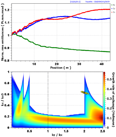
Figure 4: Case 2: Weaker transverse focusing and stability chart for $\epsilon_{z}/\epsilon_{x}=1$.

There is a real emittance transfer from the longitudinal direction into transverse - obviously induced by the third order resonance discussed in the end of Section 2. For the (conventional) energy ratio we find $T=2\to 1.3$. Note that the “independent” behaviour of transverse emittances is even more pronounced than in Fig. 3, hence Lagniel’s argument of “total correlation” between $x$ and $y$ is not supported.

We have also examined a Case 3: with $\epsilon_{z}/\epsilon_{x}=2$ and $k_{z}/k_{x}=1$ we find the expected main resonance, which leads to a fast emittance transfer during the first 10 cells already, with a final evolution $T=2\rightarrow 1.2$. Below we summarize the impact of these three simulations on the energy ratios $T$ as well as $T^{*}$:

$\begin{array}[]{cccc}&Case1&Case2&Case3\\ T&1\rightarrow 1&2\rightarrow 1.3&2\rightarrow 1.2\\ T^{*}&0.5\rightarrow 0.5&1\rightarrow 0.65&1\rightarrow 0.6\\ \end{array}$

In view of all this we find it straightforward to continue with the conventional definition of EP as $T=1$ (using $T$ defined in Eq. 1), which considers all degrees of freedom as independent. This is supported by the “splitting” of transverse emittances; furthermore by the fact that we have not found (by simulation, and avoiding extreme tune depression) a single case, where $T=1$ is subject to emittance transfer - in contrast with the assertions in Ref. [1]. The initial $T^{*}=1$ as in Case 2, instead, is unstable.

4 Lagniel’s Topics of Discussion

Based on the above findings we attempt to respond to the discussion opened in the last section of Lagniel’s paper by referring to his six points and starting with the original quotations from Ref.[1].

1- ”The linac beams are out of the EQP theorem validity limit, to apply the EQP rule designing a linac is a mistake.” It is undeniable that “true” equipartition can be applied to ergodic systems only. As we have a general difficulty to describe and measure distributions in 6D phase space, the concept of projections into 2D planes and of rms values in 2D was developed - successfully so far. In the same spirit it has become common practice to employ an rms energy ratio ($T$ in Eq.1 as a reduced, but well-defined quantity) and call the special case $T=1$ equipartitioned. Whether or not $T=1$ is a practically helpful requirement is a different question.

2- ”The application of the EQP rule does not prevent emittance exchanges induced by coupling resonances.” We find this statement is a speculative interpretation of fictitious beam footprints and not supported by our PIC simulation, also not by the stability charts. We have simulated exactly the same case as in Lagniel’s example and find that definitely no rms emittance exchange occurs (similarly for a variety of other initial emittance ratios, still equipartitioned).

3- ”Safe tunes with beam footprints out of the coupling resonances can be found when the EQP rule is not respected.” - a well-established recognition in the linac community.

4- ”The constraint imposed by the EQP rule on a linac design can lead to a non optimized beam dynamics and higher construction and operation costs.” - out of question.

5- ”The question of energy exchange / emittance transfer must be analyzed as done in circular machines (tune diagram, evaluation of the resonance excitation strength).” Authors should feel free to introduce different kinds of tune diagrams as long as they prove they are viable. We have suggested linac stability charts as they include tune depression (intensity) and tune ratios. Circular machine diagrams with $k_{z}$, $k_{x}$ (or $k_{y}$) separate may be fine, but would require a third dimension to include intensity. Actually, as we need to worry only about difference resonances of the kind $nk_{z}-mk_{x}=0$, the tune ratios suffice. The resonance driving terms are already part of the stop-band widths of the stability charts and need not to be evaluated separately.

6- ”The modern physics tools developed to characterize the level of disorder (chaos) present in nonlinear Hamiltonian systems could be applied to characterize and optimize our beams.” It should certainly be welcomed to continue using all the great tools developed in nonlinear dynamics.

Finally, we would like to comment also on Lagniel’s question at the end of his before last section: ”Why the belief in EQP did not pollute the synchrotron world?” Synchrotrons indeed have many resonances to worry about. However, as early as 1968, Montague already warned about the effect of horizontal-vertical emittance exchange by a space charge pseudo-octupole resonance on the main diagonal of the CERN Proton Synchrotron ($2Q_{x}-2Q_{y}=0$) [4]. Owed to its possible importance for high-current operation at CERN, the subject was carefully studied experimentally only much later - with excellent agreement with theory [5].

5 Final Remarks

We have shown that Lagniel’s assertions on EP and on linac resonances are not supported by PIC simulations, therefore a new approach to this topic on the ground of the presented arguments cannot be seen. Independent of this it is known since many years that there is no necessity to enforce EP, as most of the parameter space is filled by non-equipartitioned regions, where no emittance coupling is found - as shown by the linac stability charts.

It should be emphasized here that the notion of EP or non-EP in our context is based on rms quantities (emittances, tunes). Such an approach obviously cannot say anything about the question - also raised by Lagniel - of energy equipartition on surfaces in a multi-dimensional phase space. It would certainly be welcomed by everybody if future analysis would go beyond rms measures, for example including halo distributions and the question of coupling in the tail distributions, and thus open a new dimension of this problem to the scientific discussion. At the time being, however, linac designers may continue to work with their validated tools and feel free to be on EP, or not to be on EP - as long as they have a convincing reason for it.

Acknowledgment: The author is indebted to G. Franchetti for valuable discussions.

References

- [1] J.-M. Lagniel, HB2012 conference, Beijing, paper TUO3A03 (2012)
- [2] I. Hofmann, Phys. Rev. E 57, 4713 (1998).
- [3] I. Hofmann, HB2012 conference, Beijing, paper TUO3A01 (2012)
- [4] B.W. Montague, CERN-Report No. 68-38, CERN (1968)
- [5] E. Metral et al., Proc. of EPAC 2004, p. 1894 (2004)