A solenoidal synthetic field and the non-Abelian Aharonov-Bohm effects in neutral atoms

Centre for Quantum Technologies, National University of Singapore, 3 Science Drive 2, Singapore 117543

Department of Physics, University of Otago, Dunedin, New Zealand

National Institute of Education, Nanyang Technological University, 1 Nanyang Walk, Singapore 637616

Institute of Advanced Studies, Nanyang Technological University, 60 Nanyang View, Singapore 639673

Cold neutral atoms provide a versatile and controllable platform for emulating various quantum systems. Despite efforts to develop artificial gauge fields in these systems, realizing a unique ideal-solenoid-shaped magnetic field within the quantum domain in any real-world physical system remains elusive. Here we propose a scheme to generate a "hairline" solenoid with an extremely small size around 1 micrometer which is smaller than the typical coherence length in cold atoms. Correspondingly, interference effects will play a role in transport. Despite the small size, the magnetic flux imposed on the atoms is very large thanks to the very strong field generated inside the solenoid. By arranging different sets of Laguerre-Gauss (LG) lasers, the generation of Abelian and non-Abelian SU($2$) lattice gauge fields is proposed for neutral atoms in ring- and square-shaped optical lattices. As an application, interference patterns of the magnetic type-I Aharonov-Bohm (AB) effect are obtained by evolving atoms along a circle over several tens of lattice cells. During the evolution, the quantum coherence is maintained and the atoms are exposed to a large magnetic flux. The scheme requires only standard optical access, and is robust to weak particle interactions.

There is intense interest in finding new settings in which different forms of gauge fields appear. Ultracold atoms in optical lattices are ideal systems with which to achieve this goal as they offer unprecedented possibilities of emulating condensed matter and high energy physics models [10, 11, 12, 13, 14, 15, 16, 17, 18, 19, 20, 21, 22, 1, 2, 3, 4, 5, 6, 7, 8, 9]. The original magnetic and electric AB effects (type-I) are distinguished from the neutral scalar AB effect and the Aharonov-Casher effect (type-II) by the absence of any electromagnetic fields [23]. This original AB effect shows that electron wave packets are influenced by the non-zero potentials and can obtain a non-zero phase shift although they travel in field-free regions [23]. The type-I AB effect is important conceptually because it bears on three issues: whether potentials are physical quantities, whether action principles are fundamental, and the principle of locality. As such it has spawned many studies [24, 25, 26, 27, 28, 29, 30, 31, 32, 33, 34, 35, 36, 37, 38, 39]. In 1986, to overcome the issue of stray fields in the previous experiments, Toromura et al. have performed a beautiful experiment to prove the presence of the AB phase by using magnetic toroids with superconducting shields to eliminate the leakage fields [25]. In 2007, Adam et al. tested the magnetic type-I AB effect in the absence of any force for a macroscopic system [40]. Although the phase shift has been observed experimentally, the direct interference signatures in the original version of the AB effect have not yet been reported. In solid-state AB interferometer, the AB effect has also been nicely demonstrated [41]. Given the great importance of type-I AB effect as a quantum mechanical phenomenon, it is of fundamental interest to ask whether the original AB effect can be reproduced in a quantum regime and how to observe the associated interference effects. A good realization in degenerate cold gases has however so far proved elusive.

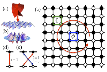
Figure 1: Schematic diagram for generating strongly localized effective Abelian and non-Abelian gauge fields with cold atoms trapped in square (a) and ring (b) lattices. The atoms can hop from one site to a neighbouring site via laser-assisted tunnelling by shinning LG lasers perpendicular to the lattice surface (a). The LG beams drive the spin-conserved transitions between two identical sublevels in neighbouring sites in (d) to generate Abelian fields, and spin-flipping transitions between two different sublevels in neighbouring sites in (e) to generate SU($2$) non-Abelian fields. The resulting magnetic flux as shown in (c) is non-zero when going around a loop (e.g., the blue square) including the laser centre which is addressed in the lattice centre and zero when the laser centre is excluded from the loop (e.g., the green square).

For the simulation of uniform or staggered gauge fields, several studies have proposed a number of methods [1, 2, 3, 4, 5, 6, 7, 8, 9], including rotation of the confining trap [10, 11, 12], using adiabatic motion of multilevel atoms in a dark-state picture [13, 14, 15], and employing spatially dependent two-photon dressing [16, 17]. In the presence of a lattice potential, schemes to generate gauge fields have been proposed using staggered-aligned states [18, 19, 20, 21] or through rotations [22]. In this work, we propose a scheme to emulate ideal-solenoid-shaped Abelian and non-Abelian gauge fields by employing LG lasers [42]. The generated magnetic field is strongly localized within a lattice cell, which allows an initially prepared coherent state of atoms to evolve along a circle without any electromagnetic field. Due to the small radius of the solenoid, the atoms can evolve along two paths within coherence time and eventually overlap so that interference occurs. At the same time, the strong strength of the magnetic field exposes the atoms to a large magnetic flux which results in a clearly visible interference signature. Besides mirroring the original AB effect relating to an Abelian gauge field, we also investigate systems exposed to a non-Abelian field which is achievable by employing more lasers. Different from the AB phase mentioned in other proposals which is accumulated from atomic evolution along four sides of a lattice cell, the AB phase here is accumulated from atomic evolution along a circle enclosing several tens of lattice cells, which makes the detection of interference more readily accessible to experiments.

Results

In this work, we consider a scheme to realize a "hairline" solenoid in both a square lattice [Fig. 1(a)] and in a ring geometry [43] [Fig. 1(b)] by employing LG-laser-assisted tunnelling. Our scheme consists of three ingredients. Firstly, atoms in different internal states are trapped in a staggered manner in a ring or a square lattice, e.g., as shown in Fig. 1(c) for a square-lattice case. The open and solid circles represent atoms in different internal states, respectively. Secondly, the depth of lattice potentials is tuned to be very large such that regular tunnelling among lattice sites is prohibited. Finally, the additional lasers with non-zero orbital angular momentum are switched on to induce tunnelling between the adjacent lattice sites.

In particular, we consider a trapping scheme with the basic principle proposed in previous works [19, 20], where two-electron atoms generally possess a spin-singlet ground state $g$ and a long-lived spin triplet excited state $e$ with a lifetime around $20$ $\mathrm{s}$ [20, 45]. The $g$ and $e$ states have opposite polarizabilities at the “anti-magic” wavelength $\lambda\simeq 1\mathrm{\mu m}$ [20], where they experience potentials with opposite signs and therefore align in a staggered manner, as shown in Fig. 1(c) for the square-lattice case. We would like to note that apart from the typical square lattice system which can be created by the interference of counter-propagating laser beams at the “anti-magic” wavelength, a ring lattice in (b) can also be created by interfering an off-resonant LG laser and a plane wave with their wavelengths chosen to be at the “anti-magic” wavelength [43]. At this stage, the lattice depth is set to be very large such that the tunnelling of atoms is strongly suppressed. As shown in Fig. 1(d), resonant LG lasers are applied to drive transitions between the $g$ and $e$ states, leading to atomic hoppings along a loop as shown in Fig. 1(c). Different values of $l$ correspond to different accumulated phase when atoms move around the loop. We consider $l=1$ and $l=0$ lasers in this work. For the former with $l=1$, it is found that the accumulated phase is $\pi$, which resembles a system where an Abelian magnetic field is applied to the atoms. For the latter with $l=0$, the accumulated phase is $0$, thus emulating a system with a zero magnetic field applied to the atoms. Moreover, when considering two sub-states in each $g$ and $e$ levels, which is shown in Fig. 1(e), an SU($2$) field can be generated by employing two LG lasers with $l=0$ and $l=1$ to drive transitions between different sub-states.

We first consider a Hamiltonian describing atoms with only one sub-state in each $g$ and $e$ levels as

$$H = \sum_{s=g,e}\int d\mathbf{r}\psi^{\dagger}_{s}(\mathbf{r})[\frac{\mathbf{\hat{p}}^{2}}{2m}+\eta_{s}V(\mathbf{r})]\psi_{s}(\mathbf{r})-\int d\mathbf{r}[d_{eg}E(\mathbf{r})^{*}e^{i\omega t}\psi^{\dagger}_{e}(\mathbf{r})\psi_{g}(\mathbf{r})+h.c.]$$ (1)

$$+\sum_{s,s^{\prime}=g,e}g_{s,s^{\prime}}\int d\mathbf{r}\psi_{s}^{\dagger}(\mathbf{r})\psi_{s^{\prime}}^{\dagger}(\mathbf{r})\psi_{s^{\prime}}(\mathbf{r})\psi_{s}(\mathbf{r}).$$

The four terms in turn give the kinetic energy, the lattice potential, the laser-assisted transition, and the interaction between atoms, respectively. Here, $\psi_{s}(\mathbf{r})$ represents the atomic field operator at position $\mathbf{r}$, $\mathbf{\hat{p}}$ is the momentum operator, and $m$ is the mass. The state-dependent sign of the lattice potential $V(r)$ is denoted by $\eta_{g}=+$ and $\eta_{e}=-$, due to the lattice lasers at the "anti-magic" wavelength. The dipole moment of the $g$-$e$ transition is labelled as $d_{eg}$, and the interaction strength is given by $g_{s,s^{\prime}}$. As shown in Fig. 1(a), the LG laser is applied perpendicular to the lattice. The amplitude of the LG laser resonant to the $g$-$e$ transition reads

$$E(\mathbf{r})=Ef_{pl}(r)e^{il\varphi}e^{i(\omega t-kz)},$$ (2)

where $f_{pl}(r)=(-1)^{p}\sqrt{\frac{2p!}{\pi(p+|l|)!}}\xi^{|l|+2}L_{p}^{|l|}e^{-\xi^{2}}$, $\xi=\frac{\sqrt{2}r}{r_{\mathrm{w}}}$, $r_{\mathrm{w}}$ is the waist of the beam, and $L_{p}^{|l|}$ are the Laguerre functions [43]. For an $N_{S}\times N_{S}$ 2D lattice, we choose $r_{\mathrm{w}}=N_{S}a/2$. The cylindrical coordinate ($r$, $\varphi$, $z$) is chosen that the longitudinal axis $z$ is along the propagation direction of the LG laser, and the labels $p$ and $l$ represent the radial and azimuthal quantum numbers, respectively.

We choose a lattice potential $V$ that is minimized at sites $\mathcal{G}=\{\text{open-circle sites}\}$ and maximized at sites $\mathcal{E}=\{\text{solid-circle sites}\}$ (see Fig. 1). In the presence of a deep lattice potential, $\psi_{s}(\mathbf{r})$ can be expressed by Wannier functions in the lowest band as $\psi_{g(e)}^{\dagger}(\mathbf{r})\simeq\sum_{j\in\mathcal{G(E)}}a_{j}^{\dagger}\omega^{*}(\mathbf{r}-\mathbf{r_{j}})$, where $\omega(\mathbf{r}-\mathbf{r}_{j})$ is the Wannier function [44]. In the numerical simulation, we approximate the Wannier functions to be Gaussion functions. Here, we have assumed that the lattice potential is symmetric for the $g$ and $e$ states. The Hamiltonian then reduces to a tight-binding model as

$$H=-\sum_{\langle i,j\rangle}(J_{i,j}a_{i}^{\dagger}a_{j}+h.c.)-J_{0}\sum_{\langle\langle i,j\rangle\rangle}(a_{i}^{\dagger}a_{j}+h.c.)+\sum_{i}\epsilon_{i}a_{i}^{\dagger}a_{i}+\frac{U}{2}\sum_{i}a_{i}^{\dagger}a_{i}^{\dagger}a_{i}a_{i}.$$ (3)

Here, the chemical potential $\epsilon_{i}$ is not relevant in terms of the gauge fields, so we treat it as uniform by tuning the lattice potential. We assume the on-site interaction strength to be identical for each site and label it as $U$. For the first hopping term, $\langle i,j\rangle$ denotes two nearest-neighbouring sites that one is in the set $\mathcal{G}$ while the other is in the set $\mathcal{E}$, between which the tunnelling is induced by the LG laser and has a strength [19, 20]

$$J_{i,j}=d_{eg}E\int d\mathbf{r}\omega^{*}(\mathbf{r}-\mathbf{r}_{i})f_{pl}(r)e^{-il\varphi}e^{ikz}\omega(\mathbf{r}-\mathbf{r}_{j}),$$ (4)

where $i\in\mathcal{G}$ and $j\in\mathcal{E}$. For the second hopping term, $\langle\langle i,j\rangle\rangle$ denotes two next-nearest-neighbouring sites, which are in the same set $\mathcal{G}$ or $\mathcal{E}$, and the corresponding tunnelling strength $J_{0}=-\int d\mathbf{r}\omega^{*}(\mathbf{r}-\mathbf{r}_{i})[\mathbf{p}^{2}/2m+\eta_{s}V(\mathbf{r})]\omega(\mathbf{r}-\mathbf{r}_{j})$. By controlling the lattice potential, the next-nearest-neighbouring tunnelling $J_{0}$ can be tuned to be much smaller than the nearest-neighbouring $J_{i,j}$, which allows us to neglect $J_{0}$ and only focus on $J_{i,j}$ in the following.

A natural property of the laser with a non-zero orbital angular momentum is a spatial-dependent phase. Since the laser is applied perpendicular to the lattice, the phase of $J_{i,j}$ will only depend on the azimuthal angle $\varphi$, as shown in Eq. (4). The phase of $J_{i,j}$ can be estimated as $J_{i,j}\propto e^{-il\varphi}$ with $\varphi$ the azimuthal angle of the midpoint between two adjacent sites $i\in\mathcal{G}$ and $j\in\mathcal{E}$. We would like to remark that the sign of the phase depends on the tunnelling direction, where for $i\in\mathcal{E}$ and $j\in\mathcal{G}$, $J_{i,j}\propto e^{il\varphi}$. Due to the vortex of the LG laser, the accumulated phase for atoms moving around a loop enclosing or excluding the laser centre are different. As a simplified illustration, we consider a centre cell of the square lattice [blue square in the centre of Fig. 1 (c)]. Here, we assume that the laser centre coincides with the centre of this cell. As a four-site circle, $\mathcal{G}$ and $\mathcal{E}$ sites appear alternatively. Without the loss of generality, we assume $\varphi=0$ along the upward direction in Fig. 1 (c). Then, for a particle moving in a counterclockwise direction, it undergoes tunnelling with phases $0$, $\frac{l\pi}{2}$, $-l\pi$, and $\frac{3l\pi}{2}$ in the four links, respectively. As a result, the accumulated phase around the centre cell is given by $0+\frac{l\pi}{2}-l\pi+\frac{3l\pi}{2}=l\pi$. By choosing an odd $l$, the accumulated phase is nontrivial, giving a non-zero gauge field within the centre cell. In the following, we will focus on the case with $l=1$ for the generation of an Abelian gauge field. As a comparison, a laser with $l=0$ will give a zero accumulated phase and therefore correspond to a zero gauge field. On the other hand, for a cell far away from the laser centre [green square in Fig. 1 (c)], the accumulated phase is always zero for any $l$, which means that a non-zero gauge field is strongly localized inside the centre cell for $l=1$, resembling a very thin solenoid. As an illustration, we consider a cell centred around $\mathbf{r}_{0}$. The laser centre is set to be the origin of the system. The coordinates of each site belonging to the cell is $\mathbf{r}=\mathbf{r}_{0}+\delta\mathbf{r}$, which gives the arimuthal angle

$$\varphi=\mathrm{arctan}(\frac{y}{x})\simeq\varphi_{0}+\frac{\mathrm{cos}\varphi_{0}\delta y-\mathrm{sin}\varphi_{0}\delta x}{r_{0}},$$ (5)

provided $r_{0}\gg a$. Here $\varphi_{0}$ is the azimuthal angle of $r_{0}$, and $a$ is the lattice constant. With $\delta x,\delta y=\pm\frac{a}{2}$, the accumulated phase is zero for a cell away from the laser centre.

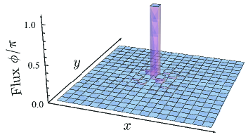
Figure 2: Numerically calculated net flux for each cell on a 2D square lattice. We have chosen $l=1$ for the LG laser, and the laser centre is addressed in the lattice centre. The flux is $\pi$ when atoms tunnel along a loop including the laser centre. Although small fluctuations appear around the centre cell, the positive and negative phases cancel each other and the total flux for a loop including the centre cell remains a value of $\pi$.

Numerical simulation for the accumulated flux $\phi_{ij}$ is shown in Fig. 2, where an $l=1$ LG laser drives the tunnelling of atoms along a loop enclosing the lattice centre that coincides with the laser centre. The flux is defined as $\phi_{i,j}=\text{arg}(J_{i,j})-\text{arg}(J_{i,j+1})+\text{arg}(J_{i+1,j+1})-\text{arg}(J_{i+1,j})$, where the tunneling strength $J_{i,j}$ is given in Eq. (4). As shown in Fig. 2, the gauge field is non-zero within only a few cells around the centre. We would like to remark that even if the centre of the laser is slightly shifted from that of the lattice, it will not affect the results significantly, although some small fluctuations may appear around the solenoid. In a similar way, an LG laser drives tunnelling of atoms which are trapped in a ring lattice. For an $l=1$ laser, the accumulated phase along the ring is $\pi$. It is straightforward to extend to the SU(2) case, where $\psi_{s}$ becomes a $2\times 1$ column matrix to include the two sub-states $g_{1}$ and $g_{2}$ ($e_{1}$ and $e_{2}$) in $g$ ($e$) level [see Fig. 1(e)]. Two laser beams with $l=0$ and $l=1$ are employed to drive $g_{1}$-$e_{2}$ and $g_{2}$-$e_{1}$ transitions, respectively. To give a unitary hopping matrix for two spins, we should choose $l=0$ and $l=1$ lasers with the same amplitude to drive the spin-flipping transitions. It is satisfied when we apply an LG mode with $p=0$, $l=1$, and a superposition of two LG modes with $p=0$, $l=0$ and $p=1$, $l=0$. The non-Abelian tunneling matrix is then given by

$$\hat{J}_{ij}=\left(\begin{array}[]{ccc}0&|J_{ij}|\\ J_{ij}&0\end{array}\right),$$ (6)

where $J_{ij}$ is given in Eq. (4).

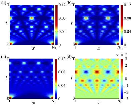
Figure 3: The time evolution of particle distributions for particles hopping around a loop formed by LG beams in a ring with $N_{\mathrm{L}}=100$ sites under a zero gauge field (a), an Abelian U(1) field (b), or a non-Abelian SU($2$) field ((c) and (d)). The particle densities are represented by the percentages of particle numbers to the total number of the initially prepared Bose-Einstein condensate. At time $t=0$, the particles are prepared around the site $x=1$. During the time period from $t=0$ to $t=T=600\hbar/E_{R}$, the fringe patterns around the opposite site $x=N_{\mathrm{L}}/2$ become completely different for the three field cases ($B=0$, U(1) and SU($2$)). Around this site, there is always a constructive interference for the $l=0$ case in (a) and a destructive interference for $l=1$ in (b). In contrast, for the non-Abelian case, the charge wave density, the sum of the two effective spins, has no unique behavior as shown in (c), and the spin wave density (d), as a difference of the two effective spins, exhibits the red-color (blue-color) component with a constructive (destructive) interference around the site $x=N_{\mathrm{L}}/2$ and a destructive (constructive) interference around the nearest neighboring area. Movies of the time evolution are available in the supplementary materials.

We would like to note the difference between our scheme and the works for continuous systems investigated in Refs. [13,14]. Although both employ laser beams with orbital angular momentum, the latter schemes deal with dark states in the electromagnetically induced transparency configuration, where the adiabatic motion of multilevel atoms is applied. In the present scheme, the necessary condition for the generation of gauge fields is a staggered distribution of different internal states and laser-assisted tunnelling. Therefore, unlike a uniform field generated in Refs. [13,14], a solenoidal field is produced here.

Type-I AB effect: To see the interference patterns, we load a Bose-Einstein condensate (BEC) initially away from the centre of the LG laser, as seen in the plot shown in Fig. 3(a)-(c) at $t=0$ for a ring-lattice case and in Fig. 4(a) for a square-lattice case. The system is then allowed to evolve under zero, Abelian and non-Abelian gauge fields. And finally the fringe patterns are measured with time. After the initial BEC state is prepared, the LG beams are switched on. At this stage, the Hamiltonian governing the time evolution is

$$H=-\sum_{\langle i,j\rangle}(J_{i,j}a_{i}^{\dagger}a_{j}+h.c.).$$ (7)

Here we have neglected the interactions between atoms. Evolutions for weakly interacting gas are analyzed in the Methods section, where the results show that the key features of the interference patterns remain robust against a weak interaction. For an LG laser with $l=1$, the accumulated phase along the circle is $\pi$. Since the atoms move along left or right path, the atoms from different paths will possess a different phase factor at the opposite site, giving a destructive interference. For an LG laser with $l=0$, the phase is always zero, which resembles the system with particles moving in the absence of any gauge field. The atoms evolving along two different paths will possess the same phase factor at the opposite site, and the interference is destructive. Therefore, the interference fringes are closely related to the phase in our scheme.

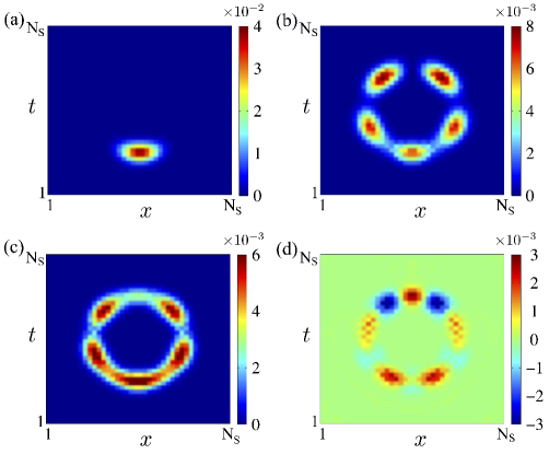
Figure 4: The time evolution of particle distributions for particles hopping around a loop formed by LG beams in a 2D square lattice with $40\times 40$ sites. At time $t=0$ as shown in (a), the particles are distributed around one site. The screenshots at time $t=4000\hbar/E_{R}$ are given for the system under an Abelian U(1) (b) or a non-Abelian SU($2$) ((c) and (d)) gauge field. The particle densities are represented by the percentages of particle numbers to the total number of the initially prepared Bose-Einstein condensate. While a destructive interference always occurs around the opposite site in the Abelian field case (b), a non-vanishing charge wave density occurs everywhere in (c) and spin waves appear in (d) with red- and blue-colored components, where the red-color (blue-color) component has a constructive (destructive) interference at the opposite side and a destructive (constructive) interference at its two neighboring area. Movies of the time evolution are available in the supplementary materials.

For a 1D ring-shaped optical lattice as illustrated in Fig. 1(b), numerical simulations for spatial distributions of particle numbers are plotted in Fig. 3, where the particle numbers are shown as a percentage of the total number in the initially prepared BEC. We have chosen the lattice site number as $N_{\mathrm{L}}=100$ and the time period $T$ as $600$ in unit of $E_{R}/\hbar$, where $E_{R}$ is the recoil energy and the typical hopping is $J\simeq 0.05E_{R}$. With $E_{R}/\hbar=2\pi\times 900$ $\mathrm{Hz}$ [20], the time scale is approximately in the range of $100$ $\mathrm{ms}$. Distinctly different interference pattens can be seen around $x=N_{\mathrm{L}}/2$ site for particles experiencing a zero magnetic field as shown in (a), an Abelian U(1) gauge field as shown in (b), and a non-Abelian SU($2$) gauge field as shown in (c)-(d). The reason for the two subfigures in the SU($2$) case is that two effective spins are involved in the SU($2$) field. We plot an effective charge wave density (the sum of densities of the two effective spins) in (c) and an effective spin wave density (the difference of densities of the two effective spins) in (d), respectively. At the $N_{\mathrm{L}}/2$ site, a destructive (constructive) interference is always seen in (b) [(a)]. Two components appear with one colored red and the other blue, where the constructive interference occurs for one type (red).

For the 2D square lattice case as illustrated in Fig. 1(a) and 1(c), we can also prepare the initial state by loading a BEC around one plaquette. For the U(1) Abelian field case as shown in Fig. 4(b), we turn on an $l=1$ laser as illustrated in Fig. 1(d), and for the non-Abelian SU($2$) field case as shown in Fig. 4 (c)-(d), we turn on two orthogonally polarized $l=0$ and $l=1$ lasers as illustrated in Fig. 1(e). Numerical simulations with time show that the angular momentum imparted by the LG beams results in a circular distributions of atoms. The particle number distribution at the opposite side of the circle from the initially prepared site again shows clear destructive interference in the case of the Abelian gauge field - the signature of the AB effect. As a concrete example, screenshots at time $t=4000\hbar/E_{R}$ are given in Fig. 4 (b)-(d). The effect is similar to the ring geometry case.

Our key result for the ring geometry is a clear demonstration of the magnetic type-I AB effect, where in the presence of an Abelian gauge field, the AB phase always induces destructive interference at the $N_{\mathrm{L}}/2$ site. Absence of any population at the $N_{\mathrm{L}}/2$ site at any time is therefore a clear signature of the Abelian AB effect. Furthermore, we demonstrate the effects of the non-Abelian gauge field in terms of the spin density waves.

Discussion

We have presented a method to generate a "hairline" solenoid with an extremely small size around 1 micrometer. Clear evidences of AB effect in the interference patterns for both Abelian and non-Abelian SU($2$) fields are obtained with a unique topological structure in both a ring geometry and a square lattice. A maximal magnetic flux is achieved as well as quantum coherence maintained during the evolution process of atoms due to the strong strength of generated magnetic field and the small radius of the solenoid. In the detection area, the interference is always constructive for the case of zero field and always destructive for the Abelian field case. For the non-Abelian field case, the spin wave density exhibits two components with a constructive or destructive interference in the detection area. The scheme requires standard optical access within the reach of current techniques, and the key conclusions are not affected by the weak particle interactions. Moreover, these effects are robust against decoherence as they are topological in origin. Consequently, they could in principle be harnessed for quantum information processing [46, 47, 48]. The technique is also straightforwardly generalized to SU($N$) gauge fields.

Methods

Interaction effect: In the main text, we have considered the non-interacting gas. A weakly interacting degenerate Bose gas can be described in the framework of the Gross-Pitaevskii equation, and now we will treat our models at the Gross-Pitaevskii level. To start with, we write down the Hamiltonian that describes interacting bosons evolving on a lattice and subjected to a gauge field:

$$H=-\sum_{\langle i,j\rangle}(J_{i,j}a_{i}^{\dagger}a_{j}+h.c.)+\frac{U}{2}\sum_{i}a_{i}^{\dagger}a_{i}^{\dagger}a_{i}a_{i}.$$ (8)

Here $a_{i}$ is a canonical Bose annihilation operator on sites of the optical lattice labeled by the integer $i$, $J_{ij}$ is the hopping amplitude, and $U$ is the interaction strength. For a weakly interacting gas, which is the typical case for the atomic gas [49], the low temperature dynamics of $H$ can be described by introducing the complex dynamical mean field variable $\psi_{i}(t)$ whose value is a measure of $\langle a_{i}(t)\rangle/\sqrt{\langle n\rangle}$. Here $\langle n\rangle$ is the average atom occupancy per lattice site. The dynamics is then described by the discrete Gross-Pitaevskii equation [50]

$$i\hbar\frac{\partial}{\partial t}\psi_{i}=\sum_{i}[-(J_{i,i+1}\psi_{i+1}+J_{i,i-1}\psi_{i-1})+\lambda J|{\psi_{i}}|^{2}\psi_{i}],$$ (9)

where $\lambda=\frac{U\langle n\rangle}{2J}$. By numerically solving the differential equations for evolutions driven by systems exposed to zero, Abelian and non-Abelian gauge fields, we have shown that the key features of the interference patterns presented here remain robust up to at least $\lambda=5$, which is easily achievable within current experimental setups.

The authors are grateful for the financial support of the National Research Foundation & Ministry of Education, Singapore.

All authors M.-X.H., W.N., D.A.W.H. and L.-C.K. contributed equally to the results.

Supplementary information is available in the online version of the paper. Reprints and permissions information is available online at www.nature.com/reprints. Correspondence and requests for materials should be addressed to huo.mingxia@physics.ox.ac.uk, david.hutchinson@otago.ac.nz, kwekleongchuan@nus.edu.sg.

The authors declare no competing financial interests.

References

- [1] Banerjee, D. et al. Atomic Quantum Simulation of Dynamical Gauge Fields Coupled to Fermionic Matter: From String Breaking to Evolution after a Quench. Phys. Rev. Lett. 109, 175302 (2012).
- [2] Zohar, E., Cirac, J. I. & Reznik, B. Simulating (2+1)-dimensional lattice QED with dynamical matter using ultracold atoms. Phys. Rev. Lett. 110, 055302 (2013).
- [3] Banerjee, D. et al. Atomic Quantum Simulation of U(N) and SU(N) Non-Abelian Lattice Gauge Theories. Phys. Rev. Lett. 110, 125303 (2013).
- [4] Gorshkov, A. V. et al. Two-orbital SU(N) magnetism with ultracold alkaline-earth atoms. Nat. Phys. 6, 289-295 (2010).
- [5] Zohar, E., Cirac, J. I. & Reznik, B. Cold-Atom Quantum Simulator for SU(2) Yang-Mills Lattice Gauge Theory. Phys. Rev. Lett. 110, 125304 (2013).
- [6] Tagliacozzo, L., Celi, A., Zamora, A. & Lewenstein, M. Optical Abelian lattice gauge theories. Annals of Physics 330, 160-191 (2013).
- [7] Tagliacozzo, L., Celi, A., Orland, P. & Lewenstein, M. Simulation of non-Abelian gauge theories with optical lattices. Nat. Commun. 4, 2615 (2013).
- [8] Goldman, N., Gerbier, F. & Lewenstein, M. Realizing non-Abelian gauge potentials in optical square lattices: an application to atomic Chern insulators. J. Phys. B: At. Mol. Opt. Phys. 46, 134010 (2013).
- [9] Zohar, E., Cirac, J. I. & Reznik, B. Quantum simulations of gauge theories with ultracold atoms: Local gauge invariance from angular-momentum conservation. Phys. Rev. A 88, 023617 (2013).
- [10] Dalibard, J., Gerbier, F., Juzeliūnas, G. & Öhberg, P. Colloquium: Artificial gauge potentials for neutral atoms. Rev. Mod. Phys. 83, 1523-1543 (2011).
- [11] Lewenstein, M. et al. Ultracold atomic gases in optical lattices: mimicking condensed matter physics and beyond. Adv. Phys. 56, 243-379 (2007).
- [12] Ho, T.-L. Bose-Einstein Condensates with Large Number of Vortices. Phys. Rev. Lett. 87, 060403 (2001).
- [13] Juzeliūnas, G., Öhberg, P., Ruseckas, J. & Klein, A. Effective magnetic fields in degenerate atomic gases induced by light beams with orbital angular momenta. Phys. Rev. A 71, 053614 (2005).
- [14] Ruseckas, J., Juzelūnas, G., Öhberg, P. & Fleischhauer, M. Non-Abelian Gauge Potentials for Ultracold Atoms with Degenerate Dark States. Phys. Rev. Lett. 95, 010404 (2005).
- [15] Juzelūnas, G. & Öhberg, P. Slow Light in Degenerate Fermi Gases. Phys. Rev. Lett. 93, 033602 (2004).
- [16] Lin, Y.-J. et al. Bose-Einstein Condensate in a Uniform Light-Induced Vector Potential. Phys. Rev. Lett. 102, 130401 (2009).
- [17] Lin, Y.-J., Compton, R. L., Jiménez-García, K., Porto, J. V. & Spielman, I. B. Synthetic magnetic fields for ultracold neutral atoms. Nature 462, 628-632 (2009).
- [18] Osterloh, K., Baig, M., Santos, L., Zoller, P. & Lewenstein, M. Cold Atoms in Non-Abelian Gauge Potentials: From the Hofstadter "Moth" to Lattice Gauge Theory. Phys. Rev. Lett. 95, 010403 (2005).
- [19] Jaksch, D. & Zoller, P. Creation of effective magnetic fields in optical lattices: the Hofstadter butterfly for cold neutral atoms. New J. Phys. 5, 56 (2003).
- [20] Gerbier, F. & Dalibard, J. Gauge fields for ultracold atoms in optical superlattices. New J. Phys. 12, 033007 (2010).
- [21] Goldman, N., Kubasiak, A., Gaspard, P. & Lewenstein, M. Ultracold atomic gases in non-Abelian gauge potentials: The case of constant Wilson loop. Phys. Rev. A 79, 023624 (2009).
- [22] Klein, A. & Jaksch, D. Phonon-induced artificial magnetic fields in optical lattices. Europhysics Lett. 85, 13001 (2009).
- [23] Aharonov, Y. & Bohm, D. Significance of Electromagnetic Potentials in the Quantum Theory. Phys. Rev. 115, 485-491 (1959).
- [24] Chambers, R. G. Shift of an Electron Interference Pattern by Enclosed Magnetic Flux. Phys. Rev. Lett. 5, 3 (1960).
- [25] Tonomura, A. et al. Evidence for Aharonov-Bohm effect with magnetic field completely shielded from electron wave. Phys. Rev. Lett. 56, 792-795 (1986).
- [26] Caprez, A., Barwick, B. & Batelaan, H. Macroscopic Test of the Aharonov-Bohm Effect. Phys. Rev. Lett. 99, 210401 (2007).
- [27] Shinohara, K., Aoki, T. & Morinaga, A. Scalar Aharonov-Bohm effect for ultracold atoms. Phys. Rev. A 66, 042106 (2002).
- [28] Webb, R. A., Washburn, S., Umbach, C. P. & Laibowitz, R. B. Observation of h/e Aharonov-Bohm Oscillations in Normal-Metal Rings. Phys. Rev. Lett. 54, 2696 (1985).
- [29] Washburn, S. & Webb, R. A. Quantum transport in small disordered samples from the diffusive to the ballistic regime. Rep. Prog. Phys. 55, 1311 (1992);
- [30] Timp, G. et al. Observation of the Aharonov-Bohm Effect for . Phys. Rev. Lett. 58, 2814 (1987).
- [31] Fuhrer, A. et al. Energy spectra of quantum rings. Nature 413, 822-825 (2001).
- [32] Fuhrer, A. et al. Energy spectra of quantum rings. Microelectron. Eng. 63, 47 (2002).
- [33] Russo, S. et al. Observation of Aharonov-Bohm conductance oscillations in a graphene ring. Phys. Rev. B 77, 085413 (2008).
- [34] Schelter, J., Recher, P. & Trauzettel, B. The Aharonov–Bohm effect in graphene rings. Solid State Comm. 152, 1411-1419 (2012), and references therein.
- [35] Bayer, M. et al. Optical Detection of the Aharonov-Bohm Effect on a Charged Particle in a Nanoscale Quantum Ring. Phys. Rev. Lett. 90, 186801 (2003).
- [36] Ribeiro, E., Govorov, A. O., Carvalho, W., Jr. & Medeiros-Ribeiro, G. Aharonov-Bohm Signature for Neutral Polarized Excitons in Type-II Quantum Dot Ensembles. Phys. Rev. Lett. 92, 126402 (2004).
- [37] Kuskovsky, I. L. et al. Optical Aharonov-Bohm effect in stacked type-II quantum dots. Phys. Rev. B 76, 035342 (2007).
- [38] Bachtold, A. et al. Aharonov–Bohm oscillations in carbon nanotubes. Nature 397, 673-675 (1999).
- [39] Zaric, S. et al. Science 304, 1129-1131 (2004).
- [40] Caprez, A., Barwick, B. & Batelaan, H. Macroscopic Test of the Aharonov-Bohm Effect. Phys. Rev. Lett. 99, 210401 (2007).
- [41] Ji, Y. et al. An electronic Mach-Zehnder interferometer. Nature 422, 415-418 (2003).
- [42] Aidelsburger, M. et al. Experimental Realization of Strong Effective Magnetic Fields in an Optical Lattice. Phys. Rev. Lett. 107, 255301 (2011).
- [43] Amico, L., Osterloh, A. & Cataliotti, F. Quantum Many Particle Systems in Ring-Shaped Optical Lattices. Phys. Rev. Lett. 95, 063201 (2005).
- [44] Jaksch, D., Bruder, C., Cirac, J. I., Gardiner, C. W., & Zoller, P. Cold Bosonic Atoms in Optical Lattices. Phys. Rev. Lett. 81, 3108 (1998).
- [45] Porsev, S. G., Derevianko A., & Fortson, E. N. Possibility of an optical clock using the SP0 transition in 171,173Yb atoms held in an optical lattice. Phys. Rev. A 69, 021403 (2004).
- [46] Leek, P. J. et al. Observation of Berry’s Phase in a Solid-State Qubit. Science 318, 1889 (2007).
- [47] Jones, J. A., Vedral, V., Ekert, A. & Castagnoli, G. Geometric quantum computation using nuclear magnetic resonance. Nature 403, 869-871 (2000).
- [48] Falci, G., Fazio, R., Palma, G. M., Siewert, J. & Vedral, V. Detection of geometric phases in superconducting nanocircuits. Nature 407, 355-358 (2000).
- [49] Zwerger, W. Mott–Hubbard transition of cold atoms in optical lattices. J. Opt. B: Quantum Semiclass. Opt. 5, S9-S16 (2003).
- [50] Polkovnikov, A., Sachdev, S. & Girvin, S. M. Nonequilibrium Gross-Pitaevskii dynamics of boson lattice models. Phys. Rev. A 66, 053607 (2002).