Quantum phases of a frustrated four-leg spin tube

Abstract

We study the ground state phase diagram of a frustrated spin-1/2 four-leg tube. Using a variety of complementary techniques, namely density matrix renormalization group, exact diagonalization, Schwinger boson mean field theory, quantum Monte-Carlo and series expansion, we explore the parameter space of this model in the regime of all-antiferromagnetic exchange. In contrast to unfrustrated four-leg tubes we uncover a rich phase diagram. Apart from the Luttinger liquid fixed point in the limit of decoupled legs, this comprises several gapped ground states, namely a plaquette, an incommensurate, and an antiferromagnetic quasi spin-2 chain phase. The transitions between these phases are analyzed in terms of total energy and static structure factor calculations and are found to be of (weak) first order. Despite the absence of long range order in the quantum case, remarkable similarities to the classical phase diagram are uncovered, with the exception of the icommensurate regime, which is strongly renormalized by quantum fluctuations. In the limit of large leg exchange the tube exhibits a deconfinement cross-over from gapped magnon like excitations to spinons.

I Introduction

Quasi one-dimensional spin systems, comprising chain, ladder and more involved magnetic structures are an active field of research thriving on a constant feedback between material synthesis, experimental investigations and theoretical predictions Dagotto1996a ; Lemmens2003 ; Batchelor2007 .

Magnetic frustration is a key issue in this field, which has experienced an upsurge of interest, starting with the discovery of $J_{1}$-$J_{2}$ chain materials, like CuGeO₃ Hase93 , followed by the investigation of spin tube compounds with an odd number $N$ of sites per unit cell, such as [(CuCl₂tachH)₃Cl]Cl₂ Schnack2004 and CsCrF₄ Manaka2009 with $N=3$, and Na₂V₃O₇ Millet1999 with $N=9$. Spin tubes with an odd number of legs and only nearest neighbor antiferromagnetic (AFM) exchange are geometrically frustrated. Because of the Lieb-Schultz-Mattis theorem the ground state of such systems is either gapless and non-degenerate, or gapped with a broken translational invariance. Indeed, for spin-1/2 tubes with $N=3$ a spin gap was found in case of identical couplings on the triangular rungs, with a transition into a gapless and translationally invariant phase at already weakly non-equivalent couplings.Fouet2006a ; Nishimoto2008a ; Ivanov2010 ; Sakai2010 ; Pujol2012 $N=3$ spin-1/2 tubes with isosceles triangle basis also show a 1/3 magnetization-plateau.Sato2007

Recently, Cu₂Cl₄$\cdot$D₈C₄SO₂ has been established as a new spin-1/2 tube with an even number of legs Garlea2008a , namely $N=4$. Tubes with $N=4$ and only nearest neighbor AFM exchange are not frustrated. However, substantial next-nearest neighbor AFM exchange, diagonally coupling adjacent legs, has been claimed for Cu₂Cl₄ $\cdot$D₈C₄SO₂, rendering also this ladder system frustrated. Inelastic neutron scattering Zheludev2008a ; Garlea2009 has revealed a strongly one-dimensional (1D) elementary excitation, which is gapped and slightly incommensurate. The former is consistent with Haldane’s conjecture Haldane1983 for 1D spin systems with an even number of spin-1/2 moments per unit cell. The latter is consistent with a frustrated exchange. Magnetic fields have been shown to stabilize the incommensurate spin correlations.Zheludev2008a ; Garlea2009

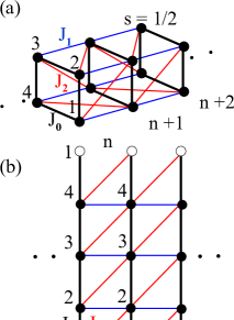
Figure 1: (color online) (a) Frustrated four-spin tube. Solid circles represent spin-$1/2$ moments. Plaquettes (bold black lines) are coupled by nearest ($J_{1}$) and next nearest ($J_{2}$) antiferromagnetic exchange, blue and red lines, respectively. On-plaquette coupling is $J_{0}$. (b) Frustrated four-spin tube unwrapped, displaying structure of an anisotropic triangular lattice on a torus.

Motivated by this, a geometrically frustrated and simplified four-spin tube (FFST) model has been introduced in Ref. Arlego2011,

$$H=\sum_{lm}J_{lm}\mathbf{S}_{l}\cdot\mathbf{S}_{m}\,,$$ (1)

with a lattice structure and exchange couplings $J_{lm}$ as shown in Fig. 1. Spin-1/2 moments are located on the solid circles and all couplings $J_{0,1,2}$ are antiferromagnetic (AFM). The FFST lattice is identical to an anisotropic triangular lattice on a torus with four site circumference.

For $J_{1,2}\ll J_{0}$, the quantum properties of the FFST can be understood in terms of weakly coupled four-spin plaquettes, which allows for series expansion in terms of $J_{1,2}$. In Ref. Arlego2011, such a series expansion has been carried out in detail regarding the one- an two-particle excitations in this restricted parameter regime. However, an understanding of the quantum phases of the FFST on a larger scale is still missing.

Therefore, in this paper we will present combined results from a large variety of complementary methods, namely, density-matrix renormalization group (DMRG), exact diagonalization (ED), series expansion (SE), Schwinger bosons mean field theory (SBMFT), and quantum Monte-Carlo (QMC) in order to explore the parameter space of the FFST. We set $J_{0}=1$, except where explicitly indicated, and denote by $L$ the tube length.

The structure of the paper is as follows. In section II we briefly summarize the phase diagram of the classical FFST. In section III we consider the quantum case focusing the discussion onto the strong and intermediate on-plaquette exchange in subsection III.1 and on the limit of very large leg exchange in subsection III.2. Section IV summarizes our picture of the FFST. For completeness we briefly summarize some of the methods used and refer to important references for them in appendix A.

II Classical phase diagram

While we are studying a quantum model in one dimension which does not allow for breaking of a continuous symmetry at zero temperature, it is nevertheless instructive to compare the quantum case considered in the following sections with a classical magnetic phase diagram of the FFST. From Ref. Arlego2011, it is known that there are four ordered regimes in which $\mathbf{S}(\mathbf{r}_{l})=S(\cos(\mathbf{Q}\cdot\mathbf{r}_{l}),\sin(\mathbf{Q}\cdot\mathbf{r}_{l}),0)$, where $\mathbf{r}_{l}$ is a lattice site:

1. $J_{2}\leqslant(1+2J_{1})/(2(J_{1}+1))$ and $J_{2}\leqslant J_{1}$: commensurate $\mathbf{Q}=(\pi,\pi)$ AFM

2. $J_{2}\geqslant(1-2J_{1})/(2(J_{1}-1))$, with $J_{1}<1$, and $J_{2}\geqslant J_{1}$: commensurate $\mathbf{Q}=(0,\pi)$ AFM

3. $J_{2}\geqslant(2J_{1}-1)/(2(J_{1}-1))$, with $J_{1}>1$: commensurate $\mathbf{Q}=(\pi,0)$ AFM

4. Two degenerate incommensurate spirals with $\mathbf{Q}(J_{1},J_{2})=\pm(2\arctan(\alpha),\pi/2)$, and $\alpha=(J_{1}+\sqrt{J_{1}^{2}+J_{2}^{2}})/J_{2}$ in the remaining region.

These are shown in Fig. 2. All classical transitions are of first order.

Figure 2: (color online) Four classical phases of the FFST with commensurate pitches $\mathbf{Q}=(\pi,\pi)$, $(\pi,0)$, $(0,\pi)$ and incommensurate regime $\mathbf{Q}(J_{1},J_{2})$ as in text.

III Quantum phases and correlation functions

In the following we gather information from various complementary methods to develop a quantum version of the phase diagram of the FFST. The dicussion is split into two subsections. The first focuses on the strong and intermediate on-plaquette exchange and comprises an analysis of the ground state energy using DMRG, SE, SBMFT, and ED, followed by an evaluation of the phase diagram from SBMFT, and finally a DMRG study of correlation funtions and structure factors. In the second subsection we analyze the spin excitations in the limit $J_{0}\rightarrow 0$ using QMC.

To begin, we note that in the quantum case and at the points $J_{1(2)}\rightarrow\infty$, $J_{2(1)}=0$ the FFST is in a Luttinger liquid (LLQ) state. Staying on either of the two axes $(J_{1(2)}\neq\infty,J_{2(1)}=0)$ , the system is unfrustrated, the inter-leg coupling is relevant, and the FFST opens a spin gap. This gapped phase is adiabatically connected to that of unfrustrated weakly coupled plaquettes $(J_{1(2)}\ll 1,J_{2(1)}=0)$ which has been studied extensively in Refs. Cabra1998, ; Kim1999, . The frustrated weakly coupled plaquette regime shows no transition between a $(\pi,\pi)$ and $(0,\pi)$ phase, rendering the diagonal line in the lower left corner of Fig. 2 a classical-only effect.

III.1 Strong and intermediate on-plaquette coupling

III.1.1 Ground state energy

A natural question arising is, how far the weakly coupled plaquette phase extends away from the $J_{1(2)}$ axes lines and if its break down is of first or second order. We check this in two ways, considering the ground state energy $e_{0}$ versus $J_{1,2}$ and the static structure factor. The results for $e_{0}$ are summarized in Fig. 3. It depicts the results from different techniques (appendix A), along two paths in parameter space. Panel (a) is along the $J_{1}$-axis, while panel (b) diagonal path $J_{1}=J_{2}$ of maximum frustration.

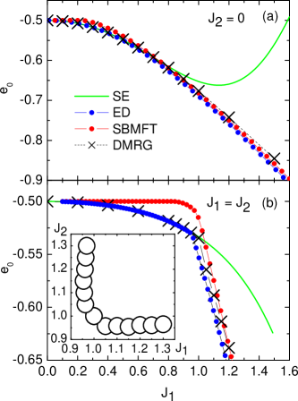
Figure 3: (color online) Ground state energy per site $e_{0}$ for $J_{0}=1$. Panel (a) $e_{0}$ vs. $J_{1}$ at $J_{2}=0$. Panel (b) $e_{0}$ vs. $J_{2}=J_{1}$. Green solid: plaquette SE at $O(7)$. Dotted blue (red): ED with L=6 and PBC (SBMFT with L=400 and PBC). Large crosses: DMRG with L=20, m=300, and OBC. Inset in (b): first order transition line in the $J_{1,2}$-plane.

Along the $J_{1}$-axis, panel (a) the energy is a smooth function. All methods are in satisfactory agreement up to $J_{1}\approx 0.7$. At this point the bare SE shown, which has been obtained up to $O(7)$ (appendix A.1), loses convergence, while the other techniques continue to agree throughout the range shown. We note that finite size effects on the DMRG and ED are expected to be small since the system is gapped.

Along the line of maximum frustration, Fig. 3 (b), the energy as obtained from DMRG and ED shows an obvious discontinuity in its first derivative at $J_{1}\approx 1$. This signals a first order quantum phase transition. Remarkably this point is rather close to the classical tricritical point, separating ($\pi,\pi$), ($0,\pi$) and spiral classical phases of Fig. 2. By construction SE based on a single unperturbed starting state is unable to detect this transition, which is consistent with Fig. 3 (b), where the SE agrees perfectly with DMRG and ED exactly up to the kink in $e_{0}$. Finally SBMFT is very close to DMRG and ED in this panel beyond the transition, however it underestimates the energy severely at smaller $J_{1}=J_{2}$. We will return to this in subsection III.1.2.

Using DMRG ground state energies, we follow the first order transition in the $J_{1,2}$-plane. This is shown in the inset of Fig. 3 (b). Apart from a very small curvature in the immediate vicinity of the transition point on the diagonal $J_{1}=J_{2}$, the plaquette phase border is composed of almost straight lines: $J_{2(1)}^{c}(J_{1(2)})\approx 1$ for $1\lesssim J_{1(2)}\lesssim 1.5$. For values of $J_{1(2)}\gtrsim 1.5$, the error on the detection of the kink from our numerical data is too large to make definite conclusions. While this is identical to previous findings in Ref. Arlego2011, , our evaluation of the static structure factor as in subsection III.1.3 shows that the first order transition is very likely to extend at least up to $J_{1(2)}\approx 5$.

In summary, ground state energy calculations seem consistent with a plaquette phase extending throughout two strips of width of order unity parallel to each of the $J_{1(2)}$-axis, at least up to intermediate $J_{1(2)}$. Finally, there are no signatures of additional first order transitions, separating a putative incommensurate and $(\pi,0)$-phase. In view of this ’missing’ second incommensurate-to-commensurate transition, we will consider also real space correlation functions and static structure factors in section III.1.3.

III.1.2 SBMFT phase diagram

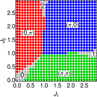
Figure 4: (color online) SBMFT phase diagram. Pitch vectors label short range spin correlations. Grey regions correspond to unphysical ’decoupled chain’ phases

Next we turn to the phase diagram as obtained from SBMFT. We use an $SU(2)$ invariant decoupling scheme described in appendix A.2 focusing on solutions with homogeneous mean fields. Apart from one Lagrange multiplier to fix the local spin, this leads to six bond parameters $B_{n=0,1,2}$ and $A_{n=0,1,2}$, one $B_{n}$ and one $A_{n}$ for each of the three non-equivalent exchange links in Fig. 1. $B_{n}$ refer to triplet, and $A_{n}$ to singlet spin correlations. Solving the self consistency Eqs. (9,10) either in the continuum limit, or, equivalently minimizing the energy of Hamiltonian (8) on sufficiently large finite FFSTs, we find the quantum phase diagram shown in Fig. 4 for $0\leqslant J_{1,2}\leqslant 3$.

First, we emphasize, that the SBMFT solutions in all of the parameter space investigated remains gapped. I.e., there is no condensation of Schwinger bosons, and correspondingly no long-range magnetic order (LRO). This is to be expected in 1D. The ’pitch’ vector labels in Fig. 4 refer to short range correlations as depicted in Fig. 5, which shows a vertical cut through the phase diagram of Fig. 4 close to $J_{1}=0$. In the ’red’ phase the AFM bond mean fields along the plaquette rungs and the diagonal $J_{2}$-links are finite, while there are ferromagnetic correlations along the $J_{1}$-links. In this sense this is a $(0,\pi)$-phase, similar to Fig. 2. The same notion applies to the $(\pi,0)$- and $(\pi,\pi)$-phase. All transitions between red, green, and blue phases in Fig. 4 are of first order.

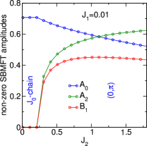
Figure 5: (color online) Non-zero bond mean field parameters within the phases of Fig. 4 versus $J_{2}$ for $J_{1}=0.01$.

Fig. 5 clearly shows, that upon lowering $J_{2}$ the FFST continuously evolves into a weakly coupled plaquette regime in the red phase. I.e., for $J_{2}\lesssim 1$, the singlet amplitudes $A_{0}$ on the plaquette rungs increase up to their maximum possible value of 1/2 at $J_{2}\approx 0.25$, while the inter-plaquette coupling amplitudes jointly decrease to zero. Qualitatively similar behavior applies to $J_{1}$ values other than that chosen in Fig. 5 within the red phase and within the green phase by interchanging $J_{1}\text{$\leftrightarrow$}J_{2}$ and $A_{2},B_{1}\leftrightarrow B_{2},A_{1}$.

However, as signaled by the grey phases in Fig. 4, and from Fig. 5, the SBMFT overestimates the stability of decoupled singlet sub-units within the FFST - such as the four-spin-plaquette. These grey phases are artifacts of the SBMFT which are reached through second order transitions. As Fig. 5 shows, SBMFT allows for small but finite parameter ranges with only one non-zero and maximized AFM bond mean field, implying that the FFST decomposes into a collection of completely decoupled $J_{0}$-, $J_{1}$-, or $J_{2}$-chains. I.e. in the grey regions the SBMFT is incapable to lower the system energy by quantum fluctuations between the latter decoupled chains. This is the reason for the poor SBMFT ground state energy in Fig. 3(b).

To conclude, also the SBMFT phase diagram is consistent with a gapped plaquette phase extending throughout two strips of width of order unity parallel to each of the $J_{1(2)}$-axis, and at least up to intermediate $J_{1(2)}$. Within this plaquette phase $(\pi,\pi)((0,\pi))$-correlations increase, as $J_{1}(J_{2})$ increase. Moreover SBMFT shows a $(\pi,0)$-phase, similar to the classical case, however with a spin gap and without long range order. We return to the latter in subsection III.2. Finally, SBMFT shows no incommensurate phase.

III.1.3 Correlation functions and static structure factor

In this section we turn to the question of a potentially incommensurate phase in the quantum case. To this end we first look at static real-space correlation functions

$$C(\mathbf{r})=\langle\mathbf{S}(\mathbf{r})\cdot\mathbf{S}(\mathbf{0})\rangle,$$ (2)

where $\mathbf{r}$ is a site on the lattice and $\langle\ldots\rangle$ the ground-state expectation value. Due to the $SU(2)$ invariance of the model, only the correlation function $C_{z}(\mathbf{r})=\langle S_{z}(\mathbf{r})S_{z}(\mathbf{0})\rangle$ needs to be considered, which satisfies $C_{z}(\mathbf{r})=C(\mathbf{r})/3$. We will contrast results from DMRG against those from SBMFT.

SBMFT results are obtained with periodic boundary conditions (PBC). For best convergence, DMRG employs open boundary conditions (OBC) along the chain. I.e., correlations depend on the reference site. To minimize edge effects, we have chosen a reference site $\mathbf{0}=(L/2,y)$ in the middle of any of the $y=(1\ldots 4)$ equivalent chains of the tube. Fig. 6, panels(b), (c), shows $C(x)$ along one of those equivalent chains, say $\mathbf{r}=(L/2-1+x,1)$ and $\mathbf{0}=(L/2,1)$.

We have focused on three particular values of $J_{1,2}$ as shown in the schematic phase diagram in panel (a). Two of them lie regions where both, the classical and the SBMFT suggest strongly commensurate correlations, and one is shortly above the first order transition of Fig. 3, where the classical state is incommensurate.

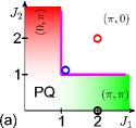
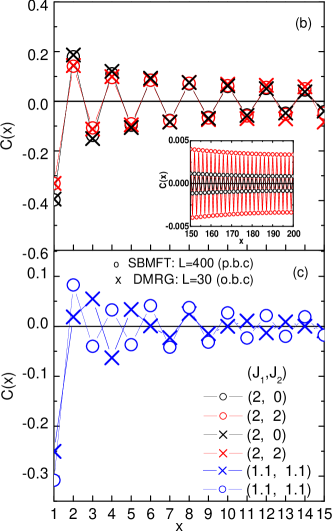
Figure 6: (color online) (a) Open colored circles: $J_{1,2}$ values chosen for panels (b), (c). PQ refers to weakly coupled plaquette phase, with predominant $(\text{$\pi$},\pi$) (green gradient) or $(0,\pi)$ (red gradient) correlations. Magenta line: first order transition evidenced from DMRG in Fig. 3(b, inset) and SBMFT in Fig. 4. (b) and (c) $C(x)=\langle\textbf{S}(x,1)\cdot\textbf{S}(L/2,1)\rangle$ vs $x$. Curve colors correspond to choices in (a). Crosses: DMRG for L=30, m=300, and OBC. Circles: SBMFT for L=400 and PBC. Inset in (b): SBMFT at large distance.

Fig. 6(b) evidences clearly commensurate correlations along the tube’s legs for the regions of the black and red open circles in Fig. 6(a) and obviously a remarkably good agreement between DMRG and SBMFT. Small deviations between DMRG and SBMFT at the ends of the chain are to be expected from the difference in boundary conditions. We have checked, that the wave vector of the commensuration is $(\pi,\pi)$($(\pi,0)$) for the black(red) circles of 6(a) by also scanning along other real-space directions on the FFST. Clearly $C(x)$ decays as a function of $x$. While the system sizes for the DMRG are too small to extract the functional form of this decay, $C(x)\sim\exp(-x/\xi)$ is found in the SBMFT, where $\xi$ is a finite correlation length related with the inverse of the energy gap. This is consistent with gapped phases and no LRO, as has already been alluded to in section III.1.2.

The situation changes drastically at the blue open circle in fig. 6(a). Here, DMRG evidences a strongly decaying, incommensurate $x$-dependence in Fig. 6(c), while SBMFT continues to display commensurate $(\pi,0)$-correlations, as to be expected from the phase diagram, Fig. 4. This proves, that SBMFT fails to produce the proper spin-correlations shortly above the first order transition out of the plaquette phase and suggests the presence of an incommensurate region also in the quantum version of the FFST.

To further corroborate this, we now calculate the static structure factor

$$S(\mathbf{Q})=\frac{1}{4L}\sum_{\mathbf{r}}e^{i\mathbf{Q}\cdot\mathbf{r}}\langle\mathbf{S}(\mathbf{r})\cdot\mathbf{S}(\mathbf{0})\rangle,$$ (3)

versus wave vector $\mathbf{Q}=(Q_{x},Q_{y})$ from our DMRG data where $\mathbf{0}=(L/2,1)$. First we consider a coarse grained set of $J_{1,2}$. The results are shown in Fig. 7. As labeled in panel (a) four values of $J_{1,2}$ are taken from regions where commensurate correlations are to be expected and two out of the vicinity of the first order transition as observed in DMRG, Fig. 3(b, inset) and SBMFT Fig. 4. Since the transverse momentum space of the tube is confined to $Q_{y}=(0,1,2,3)\pi/2$ there are four $S(Q_{x},Q_{y})$-lines for each value of $J_{1,2}$.

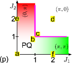
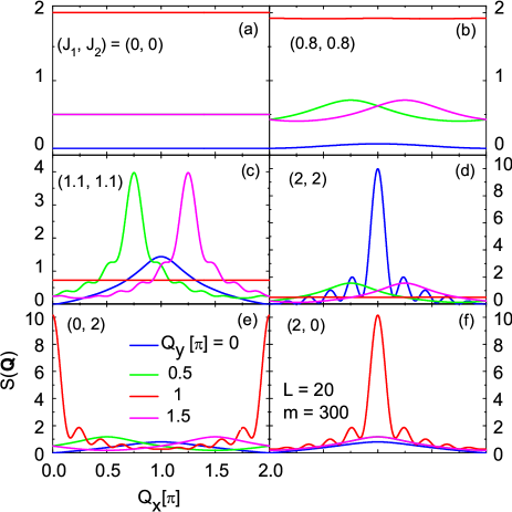
Figure 7: (color online) (p) Letters on yellow background: $J_{1,2}$ choices for panels (a)-(f). PQ refers to weakly coupled plaquette phase, with predominant $(\text{$\pi$},\pi$) (green gradient) or $(0,\pi)$ (red gradient) correlations. Magenta line: first order transition evidenced from DMRG, Fig. 3(b, inset) and SBMFT Fig. 4. Panels (a)-(f): structure factor $S(\textbf{Q})$ from DMRG (L=20, m=300, OBC) for $J_{1,2}$ as in (p). Blue, green, red, and magenta lines refer to $Q_{y}=(0,1,2,3)\pi/2$.

Fig. 7(a) exhibits a flat structure for all $Q_{y}$ modes vs. $Q_{x}$, which reflects the decoupling of the plaquettes. Moreover $S(\mathbf{Q})$ is maximum at $Q_{y,max}=\pi$ consistent with the singlet ground state on the decoupled plaquettes. Figs. 7(d,e,f) show maxima in $S(\mathbf{Q})$ at $\mathbf{Q}_{max}=(\pi,0)$, $(0,\pi)$, and $(\pi,\pi)$ respectively. This is consistent with SBMFT in Fig. 4 and also with the classical phase diagram in Fig. 2. The small oscillations around the maxima are finite size effects. On the finite system used for the DMRG calculations, the amplitude of the structure factor remains finite at $\mathbf{Q}_{max}$. From the analysis up to now, we expect no LRO on the quantum FFST, i.e. a finite value of $S(\mathbf{Q}_{max})$ for $L\rightarrow\infty$. A proof of the latter would require finite size scaling analysis, which is beyond our computational reach.

Figs. 7(b,c) describe $J_{1,2}$ values shortly below and above the first order transition of Fig. 3(b, inset), along the line of maximum frustration. Panel (b) contains a small modulation in all modes, although the plaquette phase is still evident from $Q_{y,max}=\pi$. Panel (c) however shows two-symmetric maxima at incommensurate vectors with $\mathbf{Q}_{max}=(3\pi/4,\pi/2),\,(5\pi/4,3\pi/2)$. While the $y$-component of these pitch vectors are set by the transverse quantization of the momentum space, the $x$-components are set by the quantum correlations in the FFST. Very remarkably, these $x$-components are, up to our numerical precision ($10^{-4}$), identical to the corresponding classical pitch-vectors, listed in the enumeration point 4 in section II.

Figure 8: (color online) $S(\mathbf{Q})$ from DMRG, L=30, m=300, and OBC versus $J_{1}=J_{2}$ at $\mathbf{Q}=(\pi,0)$ (blue circles), $(\pi,\pi)$ (red circles) and for the incommensurate $\mathbf{Q}_{max}=\pm(3\pi/4,\pi/2)$ (green circles). Inset: $S(\pi,\pi)$ versus $J_{1}$ at $J_{2}=0$.

Next, we discuss the DMRG structure factor in a finer grained analysis of the $J_{1,2}$ plane, along the diagonal line of maximum frustration. We have observed the occurrence of $Q_{y,max}=\pi$ with flat $Q_{x}$ dependence, characteristic of the plaquette phase, for $J_{1}=J_{2}\lesssim 0.7$ and $\mathbf{Q}_{max}=(\pi,\pi))$, still with very flat $Q_{x}$ dependence, for $0.8\lesssim J_{1}=J_{2}\lesssim 1$ (cf. Figs. 3(a,b)). We also find $\mathbf{Q}_{max}=(\pi,0)$, signaling a commensurate classical-like $(\pi,0)$ phase for $J_{1}=J_{2}\gtrsim 1.3$ (cf. Fig. 3(d)). An incommensurate phase is observed for $1\lesssim J_{1}=J_{2}\lesssim 1.3$, with $\mathbf{Q}_{max}=(3\pi/4,\pi/2),\,(5\pi/4,3\pi/2)$.

In order to describe the extent of such incommensurate region we show in Fig. 8 $S(\mathbf{Q})$ for representative momenta $\mathbf{Q}=(\pi,\pi),\,(3\pi/4,\pi/2),(\pi,0)$ in the range $J_{1}=J_{2}\in[0,1.5]$. Clearly, $S(\pi,\pi)$ is maximum and shows only a small variation in the range $J_{1}=J_{2}\in[0,1]$ (plaquette phase). At $J_{1}=J_{2}=1$, the structure factor is discontinuous. Following that, and in a small window of $1\lesssim J_{1}=J_{2}\lesssim 1.2$, $S(\mathbf{Q})$ is maximum at the incommensurate wave vector. In the vicinity of $J_{1}=J_{2}\approx 1.25$ there is a crossover from incommensurate to commensurate $(\pi,0)$ correlations. These results can be interpreted in terms of a small window of an incommensurate phase with a weak first order transition into the $(\pi,0)$-phase and a kink in the energy which is too small to be detected from the DMRG calculations in Fig. 3.

For reference the inset in Fig. 8 reports $S(\pi,\pi)$ along the $J_{1}$-axis, i.e. $J_{2}=0$, where the structure factor is maximum for any $J_{1}>0$. This plot shows a continuous increase and no signs of phase transitions in this part of parameters space. An identical observation applies to $S(0,\pi)$ along the $J_{2}$-axis, i.e. $J_{1}=0$, for all $J_{2}>0$. This is consistent with the plaquette phase being adiabatically connected with the limit of decoupled chains.

While the discussion in Fig. 8 is confined to the line of maximum frustration, we have performed similar analysis along additional lines in the $J_{1,2}$ plane. These agree with a plaquette phase in strips of width one, both, along the $J_{1}$-, and $J_{2}$-axis, as in Fig. 4, up to values of $J_{1,2}\approx 5$. This extends the range obtained from the kink in the ground state energy in Fig. 3 and Ref. Arlego2011, . Moreover, incommensurate correlations are observed beyond these strips, with $\mathbf{Q}_{max}$ slightly renormalized by quantum fluctuations with respect to the classical spiral pitch-vectors in the enumeration point 4 in section II. Unfortunately, the width of the incommensurate region decreases rapidly off from the line of maximum frustration and cannot be determined accurately enough.

To summarize, static structure factor calculations suggest that the at least close to line of maximum frustration, the plaquette phase-strips undergo a first order transition into an incommensurate phase, the extent of which is strongly decreased by quantum fluctuations with respect to the classical spiral phase. The transition between the incommensurate and the $(\pi,0)$ phase appears to be very weakly first order.

III.2 Strong leg coupling

In this subsection we consider the limit of $J_{1,2}\gg J_{0}$ by explicitly setting $J_{0}=0$. Naturally in this limit, a different normalization is required for the exchange coupling constants. We set $J_{1}=1$. For $J_{0}=0$ the FFST is unfrustrated, equivalent to an anisotropic twisted square lattice on a torus. We will use quantum Monte-Carlo, based on the stochastic series expansion, to study its properties.

III.2.1 Uniform susceptibility and spin gap

The real space arrangement of spins in the classical $(\pi,0)$ phase at $J_{1}\sim J_{2}\gg J_{0}$ is that of a spin-$2$ AFM chain. While in the quantum model the total spin per plaquette is not conserved, it is nevertheless tempting to speculate on a gap similar to that of an actual spin-2 AFM quantum chain at $J_{2}=J_{1}$. Additionally, upon reducing $J_{2}/J_{1}\text{$\rightarrow$}0$, the limit of four decoupled chains is reached, which is a LLQ and therefore shows no spin gap.

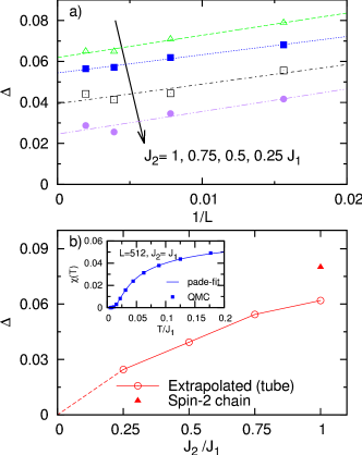
Figure 9: (color online) a) Finite size scaling for $64\leqslant L\leqslant 512$ of the spin gap for different values of $J_{2}$. b) $L=\infty$ extrapolated spin gap vs. $J_{2}$, as well as spin gap of a spin-2 chain. Inset: susceptibility vs. temperature for $L=512$ and $J_{2}=J_{1}$. Symbols: QMC data, solid curve: Padé fit, see text.

To test these assumptions, we evaluate the uniform spin susceptibility $\chi(T)$ versus temperature $T$ on systems of up to $L=512$ plaquettes for $J_{2}=1,\,0.75,\,0.5$, and $0.25J_{1}$. The case of $J_{2}=J_{1}$ is shown in the inset of Fig. 9(b). Obviously, the system has gap. The value of the gap is extracted from $\chi(T)$ by fitting the low-temperature behavior for $0.0055\leqslant T\leqslant 0.2J_{1}$ to $\chi(T)\approx e^{-\Delta/T}P_{k}^{l}(T)/T$, where $P_{k}^{l}(T)$ is a Padé approximant of order $[k,l]$. The errors of such fits - for a particular choice of the fitted temperature interval - can be made less than the QMC’s error bars, which are not shown in Fig. 9, and are of order of $10^{-6}$. Fig. 9(a) details the finite size scaling of the spin gap for $64\leqslant L\leqslant 512$. The small oscillations of the data in this plot should not be confused with QMC errors or deviations from simple scaling. Rather they are due to the particular choice of the temperature interval for the Padé fit. As is obvious from this figure, these oscillations are less than the actual finite size corrections. Finally, the main panel of fig. 9(b) proves our speculation, namely, the spin gap at $J_{2}=J_{1}$ is close to that of a spin-2 chain Grossjohann2010 and the gap decreases monotonously as $J_{2}/J_{1}\text{$\rightarrow$}0$, where, corresponding to the LLQ, $\Delta(J_{2}/J_{1}=0)=0$.

III.2.2 Dynamic structure factor

Figure 10: (color online) Contour plots of the dynamic structure factor $S(\mathbf{Q},\omega)$ from QMC & MaxEnt for systems of $L=32$ vs. $\omega$ and $Q_{x}$ at $Q_{y}=0$. Panels (a-c): for $J_{2}/J_{1}=1$, $0.5$, and $0.1$ at $T=0.25J_{2}$. Panel a) inset: $(\pi,0)$-cut of $S(\mathbf{Q},\omega)$ with labels referring to panels a)-c). Panels (d-f): for $T/J_{1}=0.5$, $0.25$, and $0.1$ at $J_{2}/J_{1}=1$. Panel d) inset: $(\pi,0)$-cut of $S(\mathbf{Q},\omega)$ with labels referring to panels d)-f).

Continuing on the analogy of a crossover from a gapped Haldane-like spin-2 AFM chain to a LLQ for $J_{2}/J_{1}$ ranging from $1$ to $0$, the dynamical structure factor of the FFST should show signatures of deconfinement from gapped ’magnon’-like modes at $J_{2}/J_{1}=1$ to a two-spinon continuum as $J_{2}/J_{1}\text{$\rightarrow$}0$.

To analyze this, we investigate the dynamic structure factor $S(\mathbf{Q},\omega)$ at frequency $\omega$, which we obtain from MaxEnt analytic continuation of imaginary time dynamic structure factor

$$S(\mathbf{Q},\tau)=\frac{1}{4L}\sum_{\mathbf{r}}e^{i\mathbf{Q}\cdot\mathbf{r}}\langle\mathbf{S}(\mathbf{r},\tau)\cdot\mathbf{S}(\mathbf{0},0)\rangle,$$

evaluated by QMC (see appendix A.3). This is shown in Fig. 10. In all of these plots $Q_{y}=0$. The absolute scales on all panels of this figure are adjusted to ensure approximately identical extent of the spectra along the $y$-axes, which allows to compare the width of the spectral contours. Turning to Fig. 10(a-c), we first note that all three contour plots display a certain broadening due to the finite temperature $T=0.25J_{1}$. We return to this in Fig. 10(d-f). Apart from that, at $J_{1}=J_{2}$ the figures show a rather sharp magnon-like mode, similar to the spectra of integer-spin Haldane chains, Meshkov1993 ; Grossjohann2010 accompanied by a marked loss of spectral weight as $Q_{x}\rightarrow 0$, which is also a typical feature of integer spin chains. Ma1992 As $J_{2}\rightarrow 0$, the spectrum starts to broaden in the vicinity of $Q_{x}=\pi$, resembling a shape very similar to that of the spinon continuum of the spin-1/2 AFM Heisenberg chain Grossjohann2009 ; Caux2011 - exactly as anticipated. The inset in Fig. 10(a) details, that although the finite temperature maximum of the dynamic structure factor does not have to coincide with the spin gap, it nevertheless decreases similar to the latter with respect to $J_{2}/J_{1}$.

Figs. 10(d-f) list the temperature dependence of $S(\mathbf{Q},\omega)$ for $J_{2}=J_{1}$. First, these panels clarify, that $T=0.25J_{1}$ is a reasonable compromise between finite size effects at $L=32$ and thermal broadening, i.e., for $T=0.1J_{1}$ the line broadening is already less than the finite-size level-spacing. Furthermore, the inset 10(d) collects cuts at $Q_{x}=\pi$, which demonstrate a rather strong temperature dependence of the zone-boundary modes of the FFST for $J_{2}\approx J_{1}\gg J_{0}$. This might be of interest in the context of similar observations Zheludev2008a for four-spin tube compound Cu₂Cl₄$\cdot$D₈C₄SO₂.

In conclusion, and even though the on-plaquette total spin is not strictly conserved in the quantum case, the FFST shows some features remarkably similar to an AFM chain with $S\approx 2$ at $J_{1}=J_{2}\gg J_{0}$, as well as a magnon-spinon deconfinement as $J_{2}/J_{1}\rightarrow 0$.

IV Discussion and Conclusions

To summarize, we have studied the quantum phases of a frustrated spin-1/2 four-leg tube using a variety of techniques: density matrix renormalization group, Quantum Monte-Carlo, Schwinger boson mean field theory, exact diagonalization and series expansions. Our main results are outlined in the tentative quantum phase diagram Fig. 11. This figure should be contrasted against the tube’s phase diagram in the classical limit, i.e. Fig. 2. While all phases in the latter are long range ordered, none of the quantum phases are.

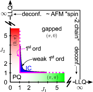
Figure 11: (color online) Quantum phase diagram of the FFST

The point $J_{1,2}=0$ hosts a gapped system of decoupled plaquettes, while at the asymptotic points $J_{1(2)}\to\infty$, $J_{2(1)}=0$ the spin tube degenerates into decoupled spin-1/2 chains in a Luttinger liquid state. The phase diagram is symmetric with respect to interchanging $J_{1}\leftrightarrow J_{2}$. On either of the two axes $J_{1(2)}=0$, the system is unfrustrated, the inter-leg coupling is relevant, and a spin gap opens. This unfrustrated weakly coupled chain regime is known to be adiabatically connected to that of the weakly coupled plaquettes.

Turning on the frustrating exchange, our results are consistent with the weakly coupled plaquette regime to survive along two strips (red and green in Fig. 11) of width of order unity, parallel to each of the $J_{1(2)}$-axis, at least up to $J_{1(2)}\approx 5J_{0}$. The system remains gapped in this region. Accordingly, our analysis of correlation functions exhibits exponential real space decay. Consistent with series expansions around $J_{1,2}=0$, the static structure factor obtained from density matrix renormalization group evolves smoothly from a flat plaquette signature around PQ in Fig. 11, into a peaked commensurate behavior along the red/green strips, parallel to each axis. The peak locations are consistent with short-range correlation remnants of the long-range order present in the classical limit of the tube this region. As for the unfrustrated four-leg tube, we expect no quantum phase transition while increasing $J_{1(2)}\rightarrow\infty$ parallel to the axis within these strips until the Luttinger liquid fixed point is reached (zig-zag marks in Fig. 11).

Perpendicular to the $J_{1,2}$-axis the plaquette regime is terminated by a line of first order transitions evidenced by those of our techniques able to detect ground state energy level crossings. The critical lines emerge approximately from the point of maximum frustration $J_{0,1,2}=1$ and run parallel to the $J_{1,2}$ axes (magenta line in Fig. 11). The numerical precision, locating the level crossing along the borders of the PQ strip, decreases away from $J_{0,1,2}=1$, indicated by the doting of the magenta line.

Beyond the first order critical line, close to the point of maximum frustration, $J_{0,1,2}=1$, DMRG shows that the plaquette phase turns into a gapped phase with short range incommensurate correlations (IC, blue in Fig. 11), analogous to the spiral phase which is found in the classical limit of the tube in this regime. Along the diagonal $1\lesssim J_{1}=J_{2}\lesssim 1.3$, the static structure factor shows a maximum approximately at the pitch vectors of the classical spiral phase. Off the diagonal, the maximum of the static structure factor is slightly shifted from the classical values. Increasing the inter-plaquette coupling, around the line $J_{1}\sim J_{2}$, the incommensurate quantum phase terminates with a very weak first order transition into a gapped commensurate ($\pi$, 0) phase, labeled by the thin black line in Fig. 11. In contrast to the PQ $(\pi,\pi)$ and $(0,\pi)$ region, the overall extent of the incommensurate region in the quantum case is strongly reduced as compared to that of the classical spiral phase.

For $J_{1,2}\gg J_{0}$, the system can be considered as approximately unfrustrated. We have investigated this regime by Quantum Monte-Carlo along the line $0<J_{2}/J_{1}\leq 1$, setting $J_{0}=0$ (black line emerging perpendicularly from the point LLQ in Fig. 11). Here calculations of the uniform susceptibility show the tube to have a gap very close to that of AFM spin-2 chains at $J_{1}=J_{2}$, while for $J_{2}/J_{1}\rightarrow 0$ the gap decreases to zero as expected for approaching the Luttinger liquid state. Evaluating the dynamic structure factor, and consistent with a crossover from a ’Haldane-like AFM spin-2 chain’ behavior at $J_{1}\sim J_{2}$ to a LLQ at $J_{2}=0$, we observe a deconfinement of the excitations turning from sharp ’magnon’ modes into a spinon continuum as $J_{2}/J_{1}\rightarrow 0$.

Finally, and due to numerical limitations in our study, it remains an open issue if the quantum IC and PQ regimes extend beyond $J_{1(2)}\sim 5$ at $J_{2(1)}\sim 1$. In this context we cannot conclude from our study whether the PQ and $(\pi,0)$ phase remain adiabatically disconnected in the quantum case or not.

V Acknowledgments

We thank D.C. Cabra for helpful discussions. MA, HDR and GR have been supported by CONICET (PIP 1691) and by ANPCyT (PICT 1426). Part of this work has been supported by the Deutsche Forschungsgemeinschaft through FOR912, Grant No. BR 1084/6-2 (WB), the European Commission through MC-ITN LOTHERM, Grant No. PITN-GA-2009-238475 (YR and WB), and the NTH School for Contacts in Nanosystems (BW and WB). WB thanks the Platform for Superconductivity and Magnetism Dresden, and the Kavli Institute for Theoretical Physics for kind hospitality. The research at KITP was supported by the National Science Foundation under Grant No. NSF PHY11-25915.

Appendix A Techniques

For completeness, this appendix provides some details and references to the methods we use in this work.

A.1 Series expansion

Our SE calculations start from the limit of isolated plaquettes. To this end we decompose the Hamiltonian of the FFST into

$$H=H_{0}+V(J_{1},J_{2}),$$ (4)

where $H_{0}$ represents decoupled plaquettes and $V(J_{1},J_{2})$ is the part of Hamiltonian that connects plaquettes via $J_{1},J_{2}$ couplings.

It is simple to show, that each plaquette has four equally spaced energy levels, which in turn renders the levels structure of $H_{0}$ to be equidistant. This allows to sort the spectrum of $H_{0}$ in a block-diagonal form, where each block is labeled by an energy quantum-number Q. In this way, Q=0 represents the ground state (vacuum), i.e., all plaquettes are in the state of minimum energy. Q=1 sector is composed by states obtained by creating (from vacuum state) one-elementary excitation (particle) on a given plaquette, and so on. It is clear that $Q\geq 2$ will be of multiparticle nature.

In general the action of $V(J_{1},J_{2})$ mixes different Q-sectors, so that the block-diagonal form of $H_{0}$ is not conserved in $H$. However, it has been shown Knetter2000a that for the present type of Hamiltonians it is possible to restore block-diagonal form by the application of continuous unitary transformations, using the flow equation method of Wegner Wegner1994a . It basically consists in transforming $H$ onto an effective Hamiltonian $H_{\mathrm{eff}}$ which is block-diagonal in the quantum number $Q$. This transformation can be achieved exactly in terms of a SE in $J_{1,2}$ leading to

$$H_{\mathrm{eff}}=H_{0}+\sum_{n,0\leq m\leq n}J_{1}^{n-m}J_{2}^{m}C_{n,m}\,.$$ (5)

Here $C_{n,m}$ are weighted products of terms in $V(J_{1},J_{2})$ which conserve the $Q$-number, with weights determined by recursive differential equations (see Ref. Knetter2000a for details).

Due to $Q$-number conservation several observables can be calculated directly from $H_{\mathrm{eff}}$ in terms of a SE in $J_{1,2}$. For systems with coupled spin-plaquettes continuous unitary transformations SE has been used for one Arlego2006a , two Arlego2008a ; Arlego2007a ; Brenig2004a ; Brenig2002aa and three Brenig2003a dimensions. For the present model we have performed $O(7)$ and $O(6)$ SE in $J_{1,2}$ for ground state energy ($Q=0$) and for $Q=1,2$ sectors, respectively. We refer for technical details about the calculation to Ref. Arlego2011 .

A.2 Schwinger bosons

Schwinger bosons Auerbach are used to represent spins at site $l$ via spinfull bosons $b_{l\sigma}^{(\dagger)}$, with $\sigma=\uparrow\downarrow$ or $\pm 1$, through $S_{l}^{\alpha}=\frac{1}{2}\sum_{\mu\nu}b_{l\mu}^{\dagger}\sigma_{\mu\nu}^{\alpha}b_{l\nu}^{\phantom{\dagger}}$, where $\sigma_{\mu\nu}^{\alpha}$ are the Pauli matrices and $\alpha=x,y,z$. The Hilbert space dimension of spin-$S$ multiplets is enforced through the constraint $\sum_{\sigma}b_{l\sigma}^{\dagger}b_{l\sigma}^{\phantom{\dagger}}$=$2S$. In terms of Schwinger bosons, the exchange interaction can be written as AA ; Auerbach

$$\mathbf{S}_{l}\cdot\mathbf{S}_{m}=\,:\hat{B}_{lm}^{\dagger}\hat{B}_{lm}^{\phantom{\dagger}}:-\hat{A}_{lm}^{\dagger}\hat{A}_{lm}^{\phantom{\dagger}}\,,$$ (6)

with the bond operators $\hat{B}_{lm}^{\dagger}$ = $\frac{1}{2}\sum_{\sigma}b_{l\sigma}^{\dagger}b_{m\sigma}^{\phantom{\dagger}}$ and $\hat{A}_{lm}$ = $\frac{1}{2}\sum_{\sigma}\sigma b_{l\sigma}b_{m-\sigma}$ and normal ordering $::$. Eqn. (6) has been used for various $SU(2)$ invariant and large $N$ factorization schemes AA ; Read1991 ; Sachdev1992 ; TGC ; Flint2009 . We follow TGC ; Flint2009 and introduce the bond mean fields $B_{lm}=\langle\hat{B}_{lm}\rangle$ and $A_{lm}=\langle\hat{A}_{lm}\rangle$, accounting for ferromagnetic (FM) and AFM correlations on equal footing. For the FFST we focus on homogeneous mean fields, implying six parameters

$$B_{n=0,1,2}\hphantom{aaaa}A_{n=0,1,2}\,,$$ (7)

where $n=0,1,2$ corresponds to the three exchange links $\mathbf{r}_{l}-\mathbf{r}_{m}$=$\mathbf{r}_{n}$=$\mathbf{R}_{y}$, $\mathbf{R}_{x}$, $\mathbf{R}_{x}+\mathbf{R}_{y}$. Fourier transformation, $b_{l\sigma}=\sum_{\mathbf{k}}e^{i\mathbf{k}\cdot\mathbf{r}_{l}}b_{\mathbf{k}\sigma}/\sqrt{N}$, leads to a bilinear mean field Hamiltonian, which can be diagonalized by standard Bogoliubov transformation, i.e. $b_{\mathbf{k}\sigma}^{\phantom{\dagger}}=u_{\mathbf{k}}a_{\mathbf{k}\sigma}^{\phantom{\dagger}}+i\,v_{\mathbf{k}}a_{-\mathbf{k}-\sigma}^{\dagger}$, with $u_{\mathbf{k}}^{2}-v_{\mathbf{k}}^{2}=1$ yielding

$$H_{\mathrm{MFT}} = \sum_{\mathbf{k}\sigma}E_{\mathbf{k}}\left(a_{\mathbf{k}\sigma}^{\dagger}a_{\mathbf{k}\sigma}^{\phantom{\dagger}}+\frac{1}{2}\right)+\sum_{n}J_{n}\left(\left|A_{n}\right|^{2}-\right.$$ (8)

$$\left.\left|B_{n}\right|^{2}\right)+2N\lambda(S+\frac{1}{2})\,,$$

where $E_{\mathbf{k}}=[\gamma_{B}(\mathbf{k})^{2}-\gamma_{A}(\mathbf{k})^{2}]^{1/2}$ is the quasiparticle dispersion with $\gamma_{A}(\mathbf{k})$ = $\sum_{n}J_{n}A_{n}\sin(\mathbf{k}\cdot\mathbf{r}_{n})$ and $\gamma_{B}(\mathbf{k})$ = $\sum_{n}J_{n}B_{n}\cos(\mathbf{k}\cdot\mathbf{r}_{n})-\lambda$. We assume $B_{n},A{}_{n}$ to be real. $\lambda$ is a Lagrange parameter to enforce the constraint on the average. Selfconsistency, i.e. $\partial\langle H_{\mathrm{MFT}}\rangle/\partial x$=0, with $x$=$A_{n},B_{n}$, and $\lambda$ leads to

$$A[B]_{n} = \frac{1}{2N}\sum_{\mathbf{k}}\frac{\gamma_{A[B]}(\mathbf{k})\sin[\cos](\mathbf{k}\cdot\mathbf{r}_{n})}{E_{\mathbf{k}}}$$ (9)

$$(S+\frac{1}{2}) = \frac{1}{2N}\sum_{\mathbf{k}}\frac{\gamma_{B}(\mathbf{k})}{E_{\mathbf{k}}}\,,$$ (10)

where eqn. (9) yields six equations for $A_{n}$ and $B_{n}$, by replacing terms with their square bracketed successors.

To obtain $A_{n},B_{n}$, and $\lambda$ we use two numerical approaches: (i) we solve eqn. (9,10) in the thermodynamic limit, and (ii) we minimize the vacuum energy of eqn. (8) with respect to $A_{n},B_{n}$, and $\lambda$ on large finite lattices with $N\leqslant 10^{4}$ sites and periodic boundary conditions. The results from both approaches agree.

In the present work we set $S=1/2$ and study the ground state energy, the quantum phases, and the spin correlation functions arising from $A_{n},B_{n}$, and $\lambda$.

A.3 Quantum Monte-Carlo

We employ the stochastic series expansion (SSE) Sandvik1992 ; Sandvik1999a ; Syljuaasen2002 , which is based on importance sampling of the high temperature series expansion of the partition function

$$Z=\sum_{\alpha}\sum_{n}\sum_{S_{n}}\frac{(-\beta)^{n}}{n!}\left\langle\alpha\right|\prod_{k=1}^{n}H_{a_{k},b_{k}}\left|\alpha\right\rangle\,$$ (11)

where $H_{1,b}=1/2-S_{i(b)}^{z}S_{j(b)}^{z}$ and $H_{2,b}=(S_{i(b)}^{+}S_{j(b)}^{-}+S_{i(b)}^{-}S_{j(b)}^{+})/2$ are spin diagonal and off-diagonal bond operators between sites $i,j$. $|\alpha\rangle=\left|S_{1}^{z},\ldots,S_{N}^{z}\right\rangle$ refers to the $S^{z}$ basis and $S_{n}=[a_{1},b_{1}][a_{2},b_{2}]\ldots[a_{n},b_{n}]$ is an index for the operator string $\prod_{k=1}^{n}H_{a_{k},b_{k}}$. This string is Metropolis sampled using diagonal updates which change the number of diagonal operators $H_{1,b_{k}}$ in the operator string and directed loop updates which perform changes of the type $H_{1,b_{k}}\leftrightarrow H_{2,b_{k}}$. For unfrustrated spin-systems the latter update comprises an even number of off-diagonal operators $H_{2,b_{k}}$, ensuring positiveness of the transition probabilities.

Evaluation of the transverse dynamic structure factor with QMC is performed in real space $i,j$ and at imaginary time $\tau$ following Ref. Sandvik1992

$$S_{i,j}\left(\tau\right)=\Bigg{\langle}\sum_{p,m=0}^{n}\frac{\tau^{m}(\beta-\tau)^{n-m}n!}{\beta^{n}(n+1)(n-m)!m!}\times\phantom{aaa}$$

$$S_{i}^{+}(p)S_{j}^{-}(p+m)\Bigg{\rangle}_{W}\leavevmode\nobreak\ ,$$ (12)

where $\langle\ldots\rangle_{W}$ refers to the Metropolis weight of an operator string of length $n$ generated by the stochastic series expansion of the partition function Sandvik1999a ; Syljuaasen2002 , and $p,m$ are positions in this string. Analytic continuation to real frequencies follows from the inversion of $S_{\perp}({\bf q},\tau)=\frac{1}{\pi}\int_{0}^{\infty}d\omega S_{\perp}({\bf q},\omega)K(\omega,\tau)$, with a kernel $K(\omega,\tau)=e^{-\tau\omega}+e^{-(\beta-\tau)\omega}$ and $\beta=1/T$, and $S_{\perp}({\bf q},\tau)=\sum_{a}e^{i{\bf q}\cdot{\bf r}_{a}}S_{a,0}(\tau)/N$.

The preceding inversion is performed using the maximum entropy method (MaxEnt), minimizing the functional $Q=\chi^{2}/2-\alpha\sigma$ bryan1 ; Jarrell1996 . Here $\chi$ refers to the covariance of the QMC data to the MaxEnt trial-spectrum $S_{\alpha\perp}({\bf q},\omega)$. Overfitting is prevented by the entropy $\sigma=\sum_{\omega}S_{\alpha\perp}({\bf q},\omega)\ln[S_{\alpha\perp}({\bf q},\omega)/m(\omega)]$. We have used a flat default model $m(\omega)$, matching the zeroth moment of the trial spectrum. The optimal spectrum follows from the weighted average of $S_{\alpha\perp}({\bf q},\omega)$ with the probability distribution $P[\alpha|S({\bf q},\tau)]$ adopted from Ref. bryan1 .

A.4 Exact diagonalization and density matrix renormalization group

All DMRG and ED calculations employ the open source packages ALPS alps and SPINPACK spinpack . We refer to their documentation. In DMRG specifications, $m$ refers to the number of states kept during sweeps.

References

- (1) E. Dagoto and T.M. Rice, Science 271, 618 (1996).
- (2) P. Lemmens, G. Güntherodt, and C. Gros, Phys. Rep. 375, 1 (2003).
- (3) M. T. Batchelor, X.W. Guan, N. Oelkers, and Z. Tsuboi. Adv. in Phys. 56, 465 (2007).
- (4) M. Hase, I. Terasaki, K. Uchinokura, Phys. Rev. Lett. 70, 3651 (1993).
- (5) J. Schnack, H. Nojiri, P. Kogerler, G.J.T. Cooper, and L. Cronin, Phys. Rev. B 70, 174420 (2004).
- (6) H. Manaka, Y. Hirai, Y. Hachigo, M. Mitsunaga, M. Ito, and N. Terada, J. Phys. Soc. Jpn., 78, 093701 (2009).
- (7) P. Millet, J. Y. Henry, F. Mila, and J. Galy, J. J. Solid State Chem. 147, 676 (1999).
- (8) J.-B. Fouet, A. Lauchli, S. Pilgram, R. M. Noack, and F. Mila, Phys. Rev. B 73, 014409 (2006).
- (9) S. Nishimoto and M. Arikawa, Phys. Rev. B 78, 054421 (2008).
- (10) N.B. Ivanov, J. Schnack, R. Schnalle, J. Richter, P. Kogerler, G.N. Newton, L. Cronin, Y. Oshima, and H. Nojiri, Phys. Rev. Lett. 105, 037206 (2010).
- (11) T. Sakai, M. Sato, K. Okamoto, K. Okunishi, and C. Itoi, J. Phys.: Cond. Mat., 22, 403201 (2010).
- (12) X. Plat, S. Capponi, and P. Pujol, Phys. Rev. B 85, 174423 (2012).
- (13) M. Sato and T. Sakai, Phys. Rev. B 75, 014411 (2007).
- (14) V. O. Garlea, A. Zheludev, L.-P. Regnault, J.-H. Chung, Y. Qiu, M. Boehm, K. Habicht, and M. Meissner, Phys. Rev. Lett. 100, 037206 (2008).
- (15) A. Zheludev, V. O. Garlea, L.-P. Regnault, H. Manaka, A. Tsvelik, and J.-H. Chung, Phys. Rev. Lett. 100, 157204 (2008).
- (16) V.O. Garlea, A. Zheludev, K. Habicht, M. Meissner, B. Grenier, L.-P. Regnault, and E. Ressouche, Phys. Rev. B 79, 060404 (R) (2009).
- (17) F.D.M. F. D. M. Haldane, Phys. Rev. Lett. 50, 1153 (1983).
- (18) M. Arlego and W. Brenig, Phys. Rev. B 84, 134426 (2011).
- (19) D. C. Cabra, A. Honecker, and P. Pujol, Phys. Rev. B 58, 6241 (1998).
- (20) E. H. Kim and J. Sólyom, Phys. Rev. B 60, 15230 (1999)
- (21) S. Grossjohann, Static and dynamic properties of low dimensional quantum spin systems, Cuvillier Göttingen, ISBN 978-3-86955-419-8 (2010).
- (22) S. V. Meshkov, Phys. Rev. B 48, 6167 (1993).
- (23) S. Ma, C. Broholm, D.H. Reich, B.J. Sternlieb, and R.W. Erwin, Phys. Rev. Lett. 69, 3571 (1992).
- (24) S. Grossjohann and W. Brenig, Phys. Rev. B 79, 094409 (2009).
- (25) J.S. Caux, H. Konno, M. Sorrell, and R. Weston, Phys. Rev. Lett. 106, 217203 (2011).
- (26) C. Knetter and G. S. Uhrig, Eur. Phys. J. B 13, 209 (2000).
- (27) F. Wegner, Ann. Phys. 506, 77 (1994).
- (28) M. Arlego and W. Brenig, Eur. Phys. J. B 53, 193 (2006).
- (29) M. Arlego and W. Brenig, Phys. Rev. B 78, 224415 (2008).
- (30) M. Arlego and W. Brenig, Phys. Rev. B 75, 024409 (2007).
- (31) W. Brenig and M. Grzeschik, Phys. Rev. B 69, 064420 (2004).
- (32) W. Brenig and A. Honecker, Phys. Rev. B 65, 140407 (R) (2002).
- (33) W. Brenig, Phys. Rev. B 67, 064402 (2003).
- (34) A. Auerbach, Interacting Electrons and Quantum Magnetism (Springer-Verlag, New York, 1994).
- (35) A. Auerbach and D.P. Arovas, Phys. Rev. Lett. 61, 617 (1988); D.P. Arovas and A. Auerbach, Phys. Rev. B 38, 316 (1988).
- (36) N. Read and S. Sachdev Phys. Rev. Lett. 66, 1773 (1991).
- (37) S. Sachdev, Phys. Rev. B 45, 12377 (1992).
- (38) H.A. Ceccatto, C.J. Gazza, and A.E. Trumper, Phys. Rev. B 47, 12329 (1993); A.E. Trumper, L.O. Manuel, C.J. Gazza, and H.A. Ceccatto, Phys. Rev. Lett. 78, 2216 (1997).
- (39) R. Flint and P. Coleman, Phys. Rev. B 79, 014424 (2009).
- (40) A. W. Sandvik, J. Phys. A 25, 3667 (1992).
- (41) A. W. Sandvik, Phys. Rev. B 59, R14157 (1999).
- (42) O. F. Syljuåsen and A. W. Sandvik, Phys. Rev. E 66, 046701 (2002).
- (43) J. Skilling and R. K. Bryan, Mon. Not. R. Astron. Soc. 211, 111 (1984).
- (44) M. Jarrell and J. E. Gubernatis, Phys. Rep. 269, 133 (1996).
- (45) A. Albuquerque, et al. (ALPS Collaboration), J. Mag. Mag. Mat. 310, 1187 (2007).
- (46) J. Schulenburg, program package SPINPACK, http://www-e.uni-magdeburg.de/jschulen/spin/