Quantum Corrections to the Hawking Radiation Spectrum

Abstract

In 1995, Bekenstein and Mukhanov suggested that the Hawking radiation spectrum was discrete if the area spectrum was quantized in such a way that the allowed areas were integer multiples of a single unit area. However, in 1996, Barreira, Carfora, and Rovelli argued that the Hawking radiation spectrum was continuous if the area spectrum was quantized with an infinite number of unit areas, as predicted by loop quantum gravity, rather than quantized with the single unit area considered by Bekenstein and Mukhanov. In this paper, contrary to what Barreira, Carfora, and Rovelli argued, we show that the Hawking radiation spectrum is still discrete when the area spectrum is quantized as loop quantum gravity predicts. In particular, we show that, for a black hole of a given temperature, the Hawking radiation spectrum is truncated at frequencies below a certain frequency.

I Introduction

Thanks to Hawking, a black hole is well known to emit particlesHawking . Hawking also argued that the radiation spectrum must follow the Planck radiation spectrum. However, strictly speaking, this is not necessarily the case as Hawking’s calculation was semi-classical rather than fully quantum. Perhaps starting from this observation, Bekenstein and Mukhanov showed that the Hawking radiation spectrum is discrete if the allowed area values are integer multiples of a single unit areaBekenstein . In this paper, by closely reviewing how Planck’s black body radiation formula is derived, we argue that the Hawking radiation spectrum is discrete not just when the allowed area values are integer multiples of a single unit area but also when the area spectrum is quantized as loop quantum gravity predictsDiscreteness ; General ; Ashtekar . This result contradicts previous arguments by Barreira et al.BCR and KrasnovKrasnov .

In Section II, we closely review the arguments that the Hawking radiation spectrum is continuous. Then, we propose a selection rule for quantum black holes, namely, that the area of the black hole can decrease only by an amount equal to a unit area upon emission of a photon. In Section III, by relating the area reduction with the energy of the emitted photon, we show that the selection rule requires that the Hawking radiation spectrum be discrete. Also in that section, we show that the Hawking radiation spectrum is truncated below a certain photon energy. We consider three different area spectra: the isolated horizon frameworkisolated ; Ghosh , the area spectrum of Tanaka and TamakiTanaka , and the area spectrum of Kong and Yoonblackholeentropy ; ToAppear . For all cases, we find that Hawking radiation is discrete. In section IV, we present an alternative, but equivalent, derivation of the relation between the area reduction and the energy of the emitted photon, which again leads to discreteness. In Section V, we derive the selection rule proposed in Section II. In Section VI, we study how our result changes if we consider logarithmic corrections to the Bekenstein-Hawking entropy. In Section VII, we compare our results with those of Refs. 13 and 14. In particular, we show that our results are clearly different. In Section VIII, we conclude our article.

II Selection rules for quantum black holes

In their articleBCR Barreira et al. notice that “the spacing of the energy levels [of a black hole] decreases exponentially with M”. They go on to say, “It follows that for a macroscopical black hole the spacing between energy levels is infinitesimal, and thus the spectral lines are virtually dense in frequency”. Their argument that for a macroscopic black hole the spacing between energy levels is infinitesimal is correct. Nevertheless, their argument that the spectral lines are virtually dense in frequency is wrong. They assume that a photon emitted from a black hole can have any energy as long as that energy can be written as the difference between the two energy values an arbitrary black hole can have. They implicitly assume that a black hole can turn into any other black hole with less energy. Similarly, they implicitly assume that a black hole can turn into any other black hole with less area.

Let’s phrase their argument mathematically. Let’s say that we have the following area eigenvalues (i.e., the unit areas):

$$A_{i}=A_{1},A_{2},A_{3},A_{4},A_{5},A_{6}....$$ (1)

Then, the black hole area $A$ must be given by the following formula:

$$A=\sum_{i}N^{i}A_{i},$$ (2)

where the $N^{i}$s are non-negative integers. Here, we can regard the black hole as having $\sum N^{i}$ partitions, each of which has one of the $A_{i}$ as its area. In this mathematical language, we can express the consideration of Barreira et al. as follows: the black hole with initial area $A_{\mathrm{int}}=\sum N^{i}_{\mathrm{int}}A_{i}$ can turn into a black hole with final area $A_{\mathrm{fin}}=\sum N^{i}_{\mathrm{fin}}A_{i}$ through the emission of photons, as long as $A_{\mathrm{fin}}<A_{\mathrm{int}}$, without any restrictions on the set of $N^{i}_{\mathrm{fin}}$.

However, if we assume that the emission of a photon is local, this is not the case. For a photon to be emitted locally, it should be emitted from a single area quantum, not simultaneously from multiple area quanta separated in space. Possibly following these considerations, Krasnov argued thatKrasnov

“Consider a quantum process in which the black hole jumps from a state $|\Gamma\rangle$ to state $|\Gamma^{\prime}\rangle$, such that the horizon area changes. This, for example, can be a process in which one of the flux lines piercing the horizon breaks, with one of the ends falling into the black hole and the other escaping to infinity (see Fig. 1b). This is an example of the emission process; the two ends of the flux line can be thought of as the two particle anti-particle quanta in Hawking’s original picture [6] of the black hole evaporation.”

Translating this into a mathematical formula, what Krasnov argues is the following:

$$\Delta A=A_{j}-A_{i}$$ (3)

for some $A_{i}>A_{j}$. In other words, the partition with area $A_{i}$ on the black hole horizon shrinks into a partition with area $A_{j}$ upon the emission of a particle because the anti-particle reaches this partition of the black hole horizon.

However, Krasnov’s argument is also troublesome. In Section V, we will explain why the selection rule should be

$$\Delta A=-A_{i}$$ (4)

for some $i$. Before doing so, we will explain the consequences of Eq. (4) in the next two sections.

III The discreteness of the Hawking radiation spectrum

From black hole thermodynamics, we know the followingHawking :

$$r=2M,$$ (5)

$$A=4\pi r^{2}=16\pi M^{2},$$ (6)

$$kT=\frac{1}{8\pi M},$$ (7)

where $A$ is the horizon area of the black hole, $T$ its temperature, $r$ its radius, and $M$ its mass, and $k$ is Boltzmann’s constant. Here, we consider the case of a Schwarzschild black hole for simplicity, but it can easily be generalized to the generic case as is done in Section IV.

Now consider the emission of a photon from the black hole. As the photon is emitted, the black hole loses energy; thus, its area decreases by $A_{i}$, the unit area predicted by loop quantum gravity as we argued in Eq. (4) in the last section. From this consideration, we can calculate $E_{photon}$, the energy of the emitted photon. First of all, the mass of the black hole decreases as

$$\Delta M=-E_{photon}$$ (8)

Then, considering Eqs. (6) and (7), the area of the black hole decreases as

$$\Delta A = 32\pi M\Delta M=-32\pi ME_{photon}$$ (9)

$$= -\frac{4E_{photon}}{kT}=-A_{i},$$

where in the last step, we assert that the black hole area must be decreased by the unit area $A_{i}$ predicted by loop quantum gravity. Therefore, we conclude the following:

$$E_{photon}=\frac{A_{i}}{4}kT.$$ (10)

Here, we see easily that the energy of the emitted photon is quantized because $A_{i}$ is quantized. In particular, as loop quantum gravity predicts that a non-zero minimum area exists, a non-zero energy exists for the photons emitted from a black hole of a given temperature.

In the case of the isolated horizon frameworkisolated ; Ghosh , the minimum area is given by $4\pi\sqrt{3}\gamma$ where $\gamma$ is the Immirzi parameter. Therefore, we have the following for the minimum energy of the emitted photon:

$$E_{min}\approx 1.49kT$$ (11)

(see Fig. 1). The Hawking radiation is truncated below this energy. The discrete frequency values allowed for Hawking radiation are represented by solid lines. In the case of the Tanaka-Tamaki scenarioTanaka , the minimum area is given by $4\pi\gamma$, where $\gamma$ is the Immirzi parameter for this case. This gives the following for the minimum energy of emitted photon:

$$E_{min}\approx 2.462kT$$ (12)

(see Fig. 2). In the case of the Kong-Yoon scenarioblackholeentropy ; ToAppear , the minimum area is given by $4\pi\sqrt{2}$. Therefore, we have the following minimum energy:

$$E_{min}\approx 4.44kT$$ (13)

(see Fig. 3).

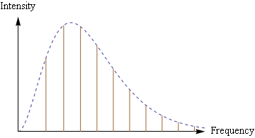
Figure 1: (Color online) Isolated horizon framework.

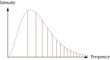
Figure 2: (Color online) Tanaka-Tamaki scenario.

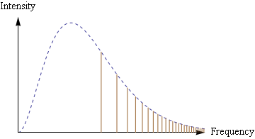
Figure 3: (Color online) Kong-Yoon scenario.

IV Alternative derivation

In this section, we present a simpler derivation. From thermodynamics, we have the following:

$$\Delta Q=T\Delta S$$ (14)

Plugging in the equalities

$$\Delta Q=-E_{photon},$$ (15)

$$\Delta S=-kA_{i}/4,$$ (16)

we recover Eq. (10).

V Griffiths’ quantum mechanics and Pathria’s statistical mechanics

In his famous textbookGriffiths , Griffiths considers a statistical mechanics problem as follows:

“Now consider an arbitrary potential, for which the one-particle energies are $E_{1},E_{2},E_{3},\cdots,$ with degeneracies $d_{1},d_{2},d_{3},\cdots$. Suppose we put $N$ particles into this potential; we are interested in the configuration ($N_{1},N_{2},N_{3},\cdots$), for which there are $N_{1}$ particles with energy $E_{1}$, $N_{2}$ particles with energy $E_{2}$ and so on. How many different ways can this be achieved?”

Then, he shows that the answer is given by the following for the case of bosons:

$$Q=\prod_{n=1}^{\infty}\frac{(N_{n}+d_{n}-1)!}{N_{n}!(d_{n}-1)!}.$$ (17)

He also explains that we have the following two conditions:

$$\sum_{n=1}^{\infty}N_{n}=N,\qquad\sum_{n=1}^{\infty}N_{n}E_{n}=E.$$ (18)

The first condition requires that the total number of particles is $N$ while the second requires that the total energy is $E$. To find the most probable configuration $(N_{1},N_{2},N_{3},\cdots)$, he maximizes $\ln Q$ as follows:

$$G\equiv\ln Q+\alpha\left[N-\sum_{n=1}^{\infty}N_{n}\right]+\beta\left[E-\sum_{n=1}^{\infty}N_{n}E_{n}\right],$$ (19)

where $G$ is to be maximized and $\alpha$ and $\beta$ are Lagrange multipliers. He concludes that

$$N_{n}=\frac{d_{n}}{e^{\alpha+\beta E_{n}}-1}.$$ (20)

Of course, in the case of photons, the number $N$ is not conserved, so we set $\alpha=0$ in Eqs. (19) and (20). Furthermore, we know $\beta=1/(kT)$, which implies

$$N_{n}=\frac{d_{n}}{e^{E_{n}/(kT)}-1}.$$ (21)

We also know (see, e.g., Section 6.4 of “Statistical Mechanics” by Pathria) that the intensity $I(E_{n})$ of photons emitted through black body radiation is given by

$$I(E_{n}) = \frac{c}{4}N_{n}A=\frac{c}{4}\frac{d_{n}}{e^{E_{n}/(kT)}-1}A$$ (22)

$$= \frac{c}{4}\frac{8\pi f^{2}df}{e^{hf/(kT)}-1}A.$$

In the last two expressions, we have substituted the density of states for the degeneracy $d_{n}$ in the numerator and written the photon energy $E_{n}$ in terms of the frequency $f$ as $hf$. Recalling that the black hole (or any black body) loses energy $hf$ upon emission of a photon with frequency $f$, we can write

$$\Delta E=-hf;$$ (23)

thus,

$$\Delta E=-E_{n}.$$ (24)

This equation shows that only the radiation associated with $E_{n}$ (i.e., a single area quanta or $n$th unit area) is possible. This can be seen better by noticing that the second equation of Eq. (18) runs parallel with Eq. (2). They are actually related by Eq. (10). Therefore, we derived Eq. (4) (i.e., $\Delta A=-A_{i}$).

Now, suppose a hypothetical case in which the area deduction is given by $\Delta A=A_{j}-A_{i}$ as Krasnov argued. In such a case, we would have $\Delta E=E_{j}-E_{i}$, which implies that the energy of the emitted photon is given by $hf=E_{i}-E_{j}$. Given this, let’s compare the black body radiation formula in this hypothetical case with Eq. (21). The denominator does not match as Eq. (21)’s denominator is $e^{E_{n}/(kT)}-1$ while Krasnov’s hypothetical one would be $e^{(E_{i}-E_{j})/(kT)}-1$. They are clearly different. Furthermore, the numerator does not match either. In the case of Eq. (21), we have the degeneracy of the $n$th quanta given as $d_{n}$. In Krasnov’s hypothetical case, whether the degeneracy should be $d_{i}$ or $d_{j}$ or $d_{i}d_{j}$ is not clear. Perhaps no consistent way exists to assign a value to the numerator such that it reduces to $d_{n}$ in the case where $E_{i}=E_{n}$ and $E_{j}=0$ but is different from $d_{n}$ when $E_{i}=E_{n}$ but $E_{j}\neq 0$. In conclusion, Krasnov’s area deduction condition is wrong as it cannot reproduce Eq. (21).

VI logarithmic corrections to the black hole entropy

In the presence of logarithmic corrections to the black hole entropy, Eq. (10), is modified. In this section, we consider the fully $SU(2)$ framework as an example. Other cases can be dealt with in a similar way. In the fully $SU(2)$ framework, we haveLivineTerno ; ENP1 ; ENP2 ; ENP3 :

$$S=\frac{A}{4}-\frac{3}{2}\ln A+O(1).$$ (25)

Given this and using Eqs. (6), (7), (14), and (15), we obtain

$$E_{photon}=\left(\frac{kT}{4}-6\pi(kT)^{3}\right)A_{i}.$$ (26)

VII Comparison with the Díaz-Polo-Fernández-Borja effect

In Refs. 13 and 14, an argument is made that loop quantum gravity effects modify the Hawking radiation spectrum, though differently from the results presented in this paper. In this section, we present their reasoning and clearly show that our results are different from theirs.

Considering the isolated horizon framework, the authors of Ref. 14 note that $\Delta A$ in Eq. (3) in our paper tends to contain integer multiples of $2.41\cdots$ more often than other values, though other values occur as well. Therefore, the corresponding photon energy associated with the values of $\Delta A$ is peaked in the spectrum around integer multiples of $2.41\cdots$ while photon energies from other values of $\Delta A$ form a continuous background. Again, from the following sentence, what they clearly considered in their paper is not our formula in Eq. (4), but Krasnov’s formula (Eq. (3) in our paper):

“In our analysis we are assuming that a black hole can undergo a transition from any configuration to any other one with the only condition that the final state belongs to a lower area band.”

They conclude their paper as follows:

“…the physical consequence that one can extract when studying the spectroscopy is not the discretization of the radiation spectrum and the appearance of a minimum emission frequency (as in the Bekenstein-Mukhanov scenario). The imprint of quantum gravity effects in Hawking radiation (for microscopic black holes) within this framework is manifested in the emergence of some equidistant brighter lines over a continuous background spectrum.”

We see here that their results are different from ours. In our case, we have the discretization of the radiation spectrum and the appearance of a minimum emission frequency, even though we used multiple unit areas as predicted by loop quantum gravity (unlike the Bekenstein-Mukhanov scenario). In our case, the discrete lines are not equidistant because the $A_{i}$ values are not equidistant nor do we have a continuous background spectrum. In conclusion, we want to note that the results refs. 13 and 14 seem to be wrong, as they are based on Eq. (3), Krasnov’s incorrect formula.

VIII Discussion and Conclusions

In this article, by closely following an elementary result explained in a quantum mechanics textbook, we showed that the Hawking radiation spectrum must be discrete and must be truncated below a certain frequency, deviating from the simple Planck radiation spectrum. We also want to note that Brian Kong and the author have given strong evidence for this phenomenon in two other papersblackholeentropy ; ToAppear ; we calculated a new area spectrum based on what we called “newer” variables and calculated the discrete Hawking radiation spectrum. Then, we approximated the new Hawking radiation spectrum as being continuous, but truncated, below a certain frequency predicted by the “newer” variables. This approximation is reasonable if you look at Fig. 3. Using this approximation, we obtained $172.87\cdots$ for a certain value associated with the strength of the Hawking radiation spectrum. We also estimated this value to be 172$\sim$173 by using a totally different method that involved statistical fitting. Again, this should be regarded as strong evidence for the discreteness of the Hawking radiation spectrum, as one would not have had this numerical agreement if there had not been a minimum frequency for the Hawking radiation spectrum. In any case, we hope that the discreteness of the Hawking radiation spectrum will be uncontroversially confirmed by detecting and measuring Hawking radiation at the Large Hadron Collider.

IX Addendum: implications on the black hole information paradox

Notice that Eq. (10) implies that the Hawking radiation is purely thermal. Therefore, the information on the objects that have fallen into a black hole cannot be retrieved through the Hawking radiation.