Design of a Unique Open-Geometry Cylindrical Penning Trap

Abstract

The Texas A&M University Penning Trap facility is an upcoming ion trap that will be used to search for possible scalar currents in $T=2$ superallowed $\beta$-delayed proton decays, which, if found, would be an indication of physics beyond the standard model. In addition, TAMUTRAP will provide a low-energy, point-like source of ions for various other applications at the Cyclotron Institute. The experiment is centered around a unique, compensated cylindrical Penning trap that employs a specially optimized $\mathrm{length}/\mathrm{radius}$ ratio in the electrode structure that is not used by any other facility. This allows the geometry to exhibit an unprecedented 90 mm free radius, which is larger than in any existing trap, while at the same time remaining a tractable overall length. The trap geometry was designed from first principles to be suitable for a wide range of nuclear physics experiments. In particular, the electrode structure is both “tunable” and “orthogonalized”, which allows for a near quadrupole electric field at the trap center, a feature necessary for performing precision mass measurements.

1 Introduction

Low energy precision $\beta$-decay experiments have proven to be an excellent compliment to high energy physics for placing new constraints on physics beyond the standard model (SM) [1, 2, 3]. Up to this point, it has been possible to explain the results from such experiments by a time reversal invariant $V-A$ interaction displaying a maximal violation of parity; however, more precise measurements of $ft$ values [4, 5] and correlation parameters [6] in particular $\beta$-decays can serve to test for the presence and properties of any non-SM processes that may occurr in such interactions.

1.1 Motivation

The initial experimental program at the upcoming Texas A&M University Penning Trap (TAMUTRAP) facility will seek to improve the limits on non-SM processes in the weak interaction, in particular scalar currents, by measuring the $\beta-\nu$ correlation parameter, $a_{\beta\nu}$, for $T=2$, $0^{+}\rightarrow 0^{+}$ superallowed $\beta$-delayed proton emitters (the generic decay scheme is shown in Fig. 1, and the preliminary list of nuclei to be studied is outlined in Table 1).

Figure 1: Decay scheme for a generic $T=2$, $0^{+}\rightarrow 0^{+}$ superallowed $\beta$-delayed proton decay.

The general $\beta$-decay rate with no net polarization or alignment is given by [7]:

$$\frac{d^{5}\Gamma}{dE_{e}d\Omega_{e}d\Omega_{\nu}}\propto 1+\frac{p_{e}}{E_{e}}a_{\beta\nu}\cos{\theta_{\beta\nu}}+b\frac{m_{e}}{E_{e}},$$ (1)

where, $E_{e}$, $p_{e}$, and $m_{e}$ are the energy, momentum, and mass of the $\beta$, $\theta_{\beta\nu}$ is the angle between the $\beta$ and $\nu$, and $b$ is the Fierz interference coefficient. Thus, it is possible to determine the $\beta-\nu$ correlation parameter by means of an experimental measurement of the angular distribution between the $\beta$ and $\nu$. For the strict $V-A$ interaction currently predicted by the SM (in pure Fermi decays) the $\beta-\nu$ angular distribution should yield a value for $a_{\beta\nu}$ of exactly 1. Any admixture of a scalar current to the predicted interaction, a result of particles other than the expected $W^{\pm}$ being exchanged during the decay, would result in a measured value of $a_{\beta\nu}<1$.

Nuclide	Lifetime (ms)	$E_{p}$ (MeV)	$R_{L}$ (mm)
20Mg	$137.05$	$4.28$	$42.7$
24Si	$147.15$	$3.91$	$40.8$
28S	$180.33$	$3.70$	$39.7$
32Ar	$141.38$	$3.36$	$37.8$
36Ca	$141.15$	$2.55$	$33.0$
40Ti	$72.13$	$3.73$	$39.9$
48Fe	$63.48$	$1.23$	$22.9$

Table 1: The $T=2$ nuclei that will compose the initial experimental program measuring $a_{\beta\nu}$. The Larmour radii, $R_{L}$, for the ejected protons of interest (having energy $E_{p}$) shown are calculated for the 7 T magnetic field of TAMUTRAP.

TAMUTRAP will observe this angular distribution between $\beta$ and $\nu$ for $\beta$-delayed proton emitters in order to take advantage of the benefit these particular decays have on the experimental procedure. In such a case, the $\beta$-decay yields a daughter nucleus that is unstable, and can result in the subsequent emission of a proton with significant probability. As discussed in [6], the great advantage to utilizing $\beta$-delayed proton emitters for such a study is that this proton energy distribution contains information about $\theta_{\beta\nu}$. If the $\beta$ and $\nu$ are ejected from the parent nucleus in the same direction, they will impart a larger momentum kick to the daughter nucleus, which will be inherited by the proton. Conversely, if the $\beta$ and $\nu$ are emitted in opposite directions, this momentum kick is reduced. By measuring the proton energy distribution at TAMUTRAP the value of $a_{\beta\nu}$ will be deduced, which can then indicate the existence of scalar currents in these decays [7].

1.2 Cylindrical Traps

A cylindrical Penning trap geometry allows for efficient access to the trapped ions, a large trapping volume compared to a hyperboloid trap geometry, and an electric field that can be described analytically, which is of particular importance during the design process. Additionally, cylindrical electrodes are more easily manufactured with higher precision. For these reasons, Penning traps with a cylindrical geometry have been widely employed in nuclear physics research experiments ranging from precision mass measurements [8] to the production of anti-hydrogen [9].

Precision $\beta$-decay experiments are well served by a cylindrical geometry due to the fact that the magnetic field employed to trap the ions radially may simultaneously be used to contain charged decay products [10] such as $\beta$’s and protons with up to $4\pi$ acceptance in an appropriately designed trap. The strong magnetic radial confinement in combination with the weak electrostatic axial confinement direct the decay products of interest to either end of the trap for detection with negligible affect on the energy of the particles. At the same time, features of a cylindrical trap geometry can be useful for other nuclear physics experiments, such as maintaining a line of sight to the trap center for spectroscopy, an easily “tunable” and “orthogonalized” electric field for experiments requiring a harmonic potential (such as mass measurements), and unrivaled access to the trapped ions.

2 Design of TAMUTRAP

For the reasons mentioned in §1.2, a cylindrical geometry has been chosen for the TAMUTRAP measurement Penning trap [11]. This particular geometry has been optimized to create a design that is suitable both for the precision $\beta$-decay experiments of interest, as well as a wide range of nuclear physics experiments as discussed. Specifically, the trap must display a large-bore for containment of decay products, it should allow for the placement of biased detectors at both ends for observation of these products, and it should exhibit a “tunable” and “orthogonalized” geometry in order to achieve a harmonic electric field.

2.1 Large-bore

For $\beta-\nu$ correlation measurements, the trap must have a free diameter large enough to contain the decay products of interest within the electrodes via the Lorentz force imposed by the trapping magnetic field. The initial program of measuring $a_{\beta\nu}$ will investigate the $T=2$ nuclei shown in Table 1, by observing the proton energy distribution. To fully contain protons of interest with full $4\pi$ acceptance the trap radius is set to twice the Larmour radius of the most energetic expected proton within the 7 T magnetic field provided by the Agilent 7T 210 ASR magnet [12]. The trap radius was chosen to be 90 mm, which will fully contain protons of up to 4.75 MeV. This radius will be the largest of any existing Penning trap and will easily contain the protons of interest, as well as the less magnetically rigid $\beta$’s, for the initial $a_{\beta\nu}$ studies.

2.2 Endcaps

The other primary requirement for performing the mentioned correlation measurements is that the design must ultimately accommodate position sensitive strip detectors at either end of the trap. The charged decay products ($\beta$, $p$, daughter) exhibit Larmour precession contained completely within the bore of the Penning trap until they are detected by such a detector. These detectors have been simulated separately as disk-shaped “endcap electrodes.” Such an approximation satisfies the need to bias the detectors at some arbitrary potential not necessarily equal to that of the hollow cylindrical end electrodes. The impact of the endcap electrodes on the solution to the complete electric field is discussed in detail in §2.3.

2.3 Tunable

A priority for the TAMUTRAP facility is to attain a very good quadrupole field at the center of the measurement Penning trap. To achieve this, the trap design must be “tunable”, that is, it must make use of compensation electrodes that serve to adjust the field shape. Other cylindrical traps [13, 14] already employ tunable geometries; however, these configurations were not suitable for TAMUTRAP due to the large-bore requirement: enlarging such geometries (which does not inherently affect the field shape if all features are scaled appropriately), results in a trap too long to fit within the available 7 T magnet. In addition, the analytic solutions of the electric field used to design these existing traps [15] directly employ long-endcap approximations, which makes a new design utilizing the existing field calculations not applicable to the short-endcap / large-bore requirement necessitated by the envisioned TAMUTRAP experimental program.

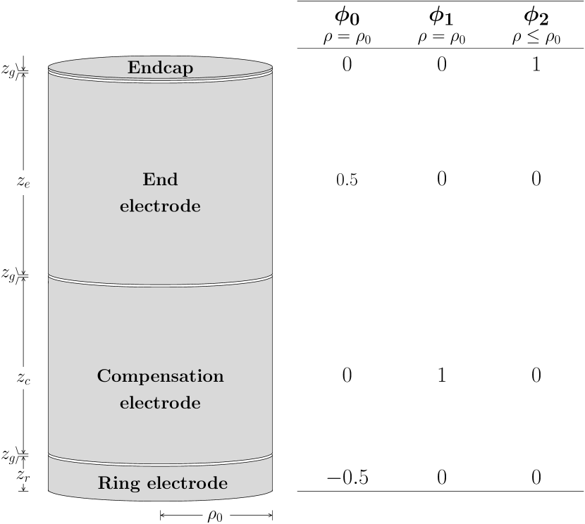
Figure 2: The trap geometry and boundary conditions used in the analytic solution.

For these reasons, a new analytic solution for a short-endcap, tunable Penning trap was derived from first principles, in part following the discussion in Ref. [15]. The contribution to the potential due to the various electrodes (Fig. 2) can be found by noting that any potential may be expanded in terms of the Legendre polynomials, $P_{k}$, the potential depth, radius from the trap axis, and characteristic trap distance [15] , $V_{0}$, $r$, and $d$, respectively, and the expansion coefficients, $C_{k}$ (here $k$ is even due to symmetry across the trapping plane):

$$V =\frac{1}{2}V_{0}\sum_{\begin{subarray}{c}k=0\\ k\ \mathrm{even}\end{subarray}}^{\infty}C_{k}\left(\frac{r}{d}\right)^{k}P_{k}(\cos{\theta}),$$ (2)

with

$$d =\sqrt{\tfrac{1}{2}\left[(z_{r}+z_{g}+z_{c}+z_{g})^{2}+\tfrac{1}{2}\rho_{0}^{2}\right]}.$$ (3)

By superposition, the potential at the trap center may also be written as a sum of the potentials of each of the contributing electrodes:

$$V=V_{0}\phi_{0}+V_{1}\phi_{1}+V_{2}\phi_{2}.$$ (4)

Here, $\phi_{0}$ is due to the boundary conditions generated by the ring and end electrodes (the primary potential well), and $\phi_{1}$ and $\phi_{2}$ are from the compensation and endcap (detector) electrodes respectively (Fig. 2), while the $V_{i}$’s are the potentials at which these electrodes are held. Each of the $\phi$’s can in turn be expanded in Legendre polynomials and substituted back into Eq. 4, which yields the simple result:

$$C_{k}=D_{k}+E_{k}\frac{V_{1}}{V_{0}}+F_{k}\frac{V_{2}}{V_{0}},$$ (5)

where $D_{k}$, $E_{k}$, and $F_{k}$ are the individual expansion coefficients due to the ring and end electrodes, compensation electrodes, and endcap (detector) electrodes respectively, and must be solved for individually. $D_{k}$ and $E_{k}$, which are due to hollow cylinder shaped electrodes, can be found by expanding $\phi_{0}$ and $\phi_{1}$ in Bessel functions, $J_{\alpha}$. After applying the periodic boundary condition in $z$, $\phi(z)=\phi(-z)$, it can be found that

$$\phi_{i}=\sum_{n=0}^{\infty}A_{n}J_{0}(\imath k_{n}\rho)\cos{(k_{n}z)},$$ (6)

where $A_{n}$ is an additional expansion coefficient. Here $k_{n}$ is due to the periodic boundary condition, and is given by

$$k_{n}=\frac{(n+\frac{1}{2})\pi}{z_{\mathrm{tot}}},$$ (7)

where $z_{\mathrm{tot}}=z_{r}+z_{c}+z_{e}+3z_{g}$. Setting Eq. 6 equal to the expansion in Legendre polynomials (Eq. 2) allows one to solve for the expansion coefficients of the Legendre polynomials by equating the two along $\hat{z}$. This results in the following solutions:

$$D_{k} =\sum_{n=0}^{\infty}\frac{2A_{n}^{D}d^{k}k_{n}^{k}(-1)^{k/2}}{k!}$$

$$E_{k} =\sum_{n=0}^{\infty}\frac{2A_{n}^{E}d^{k}k_{n}^{k}(-1)^{k/2}}{k!}.$$

The coefficients $A_{n}^{i}$ are subsequently determined by applying the appropriate boundary conditions (Fig. 2) along with the orthogonality of cosine, yielding

$$A_{n}^{D} =\frac{(-1)^{n}-\sin[k_{n}(z_{r}+z_{g}+z_{c}+z_{g})]-\sin(k_{n}z_{r})}{k_{n}z_{\mathrm{tot}}J_{0}(\imath k_{n}\rho_{0})}$$

$$A_{n}^{E} =\frac{2\big{(}\sin[k_{n}(z_{r}+z_{g}+z_{c})]-\sin[k_{n}(z_{r}+z_{g})]\big{)}}{k_{n}z_{\mathrm{tot}}J_{0}(\imath k_{n}\rho_{0})}.$$

The contribution to the potential from the endcap electrodes must be handled differently. Here $\phi_{2}$ is defined at $z_{\mathrm{tot}}$ for any radius less than $\rho_{0}$. After simplifying due to the cylindrical symmetry of the system, $\phi_{2}$ can be written:

$$\phi_{2}=\sum_{n=0}^{\infty}J_{m}(k_{0n}\rho)e^{k_{0n}z}B_{n},$$ (10)

where, $k_{mn}$ is related to $x_{mn}$, the $n$^th zero of the $m$^th Bessel function as in

$$k_{mn}=\frac{x_{mn}}{\rho_{0}}.$$ (11)

$B_{n}$ can now be determined through the application of appropriate boundary conditions (see Fig. 2) and the Bessel function orthogonality relation, giving

$$B_{n}=\frac{2e^{-k_{0n}z_{\mathrm{tot}}}}{x_{0n}J_{1}(x_{0n})}.$$ (12)

Taking into account both endcaps (at $\pm z$) yields the complete formulation of the potential due to the endcaps at any $z$:

$$\phi_{2}=\frac{V_{2}}{2}\left[\sum_{n=1}^{\infty}J_{0}\left(\frac{x_{0n}}{\rho_{0}}\rho\right)e^{z\frac{x_{0n}}{\rho_{0}}}\frac{2e^{-k_{0n}z_{\mathrm{tot}}}}{x_{0n}J_{1}(x_{0n})}\right.\\ +\left.\vphantom{\sum_{n=1}^{\infty}J_{0}}\sum_{n=1}^{\infty}J_{0}\left(\frac{x_{0n}}{\rho_{0}}\rho\right)e^{-z\frac{x_{0n}}{\rho_{0}}}\frac{2e^{-k_{0n}z_{\mathrm{tot}}}}{x_{0n}J_{1}(x_{0n})}\right].$$ (13)

This result for the potential was subsequently Taylor expanded using Mathematica [16], yielding coefficients which may be referred to here by $T_{k}$. Setting the result from the expansion equal to the potential expanded in Legendre polynomials along the $z$-axis and equating terms yields the final result for the coefficients $F_{k}$:

$$F_{k}=V_{0}T_{k}d^{k}.$$ (14)

All expansion coefficients from Eq. 5 have now been completely defined, and the electric field at the trap center can be specified to arbitrary precision. By construction, it is easy to characterize the components of this field, which allows for a straightforward optimization.

2.4 Orthogonal

For certain experiments (such as precision mass measurements), it is crucial to be able to tune out the anharmonic terms ($C_{\geq 4}\rightarrow 0$) of the electric field during the course of a measurement without affecting the harmonic ($C_{2}$) component of the field. In order to achieve this for TAMUTRAP, the procedure discussed in Ref. [15] was followed.

The strength of the dominant anharmonic term for the superposition of the electric fields is given by the coefficient $C_{4}$, and the second most dominant contribution comes from $C_{6}$, which has an affect on the shape of the electric field smaller than $C_{4}$ by a magnitude of ${(r/d)}^{2}$ (where $r$ is that radius of ion motion and $d$ is the characteristic trap dimension) [15]. These coefficients are determined, in turn, by the anharmonic contributions from the constituent electrodes, that is, $D_{4}$, $D_{6}$, $E_{4}$, $E_{6}$, $F_{4}$, and $F_{6}$. $C_{4}$ may always be tuned out by adjusting the potential on the compensation electrodes until the field is essentially harmonic. For a general geometry, however, this procedure will affect the value of $C_{2}$. Since only the potentials of the compensation electrodes are adjusted in this process, it is possible to eliminate this affect by requiring that $E_{2}=0$, that is that the compensation electrodes have no influence on the harmonic term of the superposition, $C_{2}$.

The expansion coefficient $E_{2}$, which is a function of the entire geometry, was minimized using the analytic solution derived above. To do this, the constraints imposed by other considerations (trap bore, assembly considerations, etc.) were first imposed. This left three free parameters: ring electrode length, compensation electrode length, and end electrode length. Ring electrode length and end electrode length were chosen in order to both minimize $C_{6}$ and achieve a large tunability with respect to $C_{4}$, where tunability is described in Ref. [17]:

$$\text{Tunability}=V_{0}\frac{dC_{4}}{dV_{1}}.$$ (15)

After determining the ring and end electrode lengths in this way, $E_{2}$ was minimized with respect to the remaining parameter, the compensation electrode length, thereby “orthogonalizing” the geometry. Since $E_{2}$ changes sign when scanning over electrode length, it was possible to choose a geometry that resulted in an arbitrarily small value for $E_{2}$.

3 TAMUTRAP

Performing the optimization as discussed above resulted in the geometry shown in Fig. 3. The trap radius is 90 mm, which is larger than in any existing Penning trap. The ring electrode length is 29.17 mm, the compensation electrode length is 71.36 mm, the end electrode length is 80.00 mm, and 0.50 mm gaps have been accounted for. This geometry results in a $\mathrm{length}/\mathrm{radius}$ ratio of $l/r_{0}=3.72$. A good quadrupole field ($C_{4}=-6.8\times 10^{-6}$, $C_{6}=6.2\times 10^{-6}$) has been calculated to be achievable with compensation electrodes set to $V_{1}=-0.373V_{0}$ (where $V_{0}$ is the primary trap depth). The analytic expansion of the electric field around the trap center up to $C_{8}$ is shown in Table 2. Changing the voltage on the endcap electrodes (detectors) will adjust the predicted tuning (compensation) voltage; however, the trap will always remain “tunable” and “orthogonalized” since the contributions to the potential for each electrode are independent by superposition.

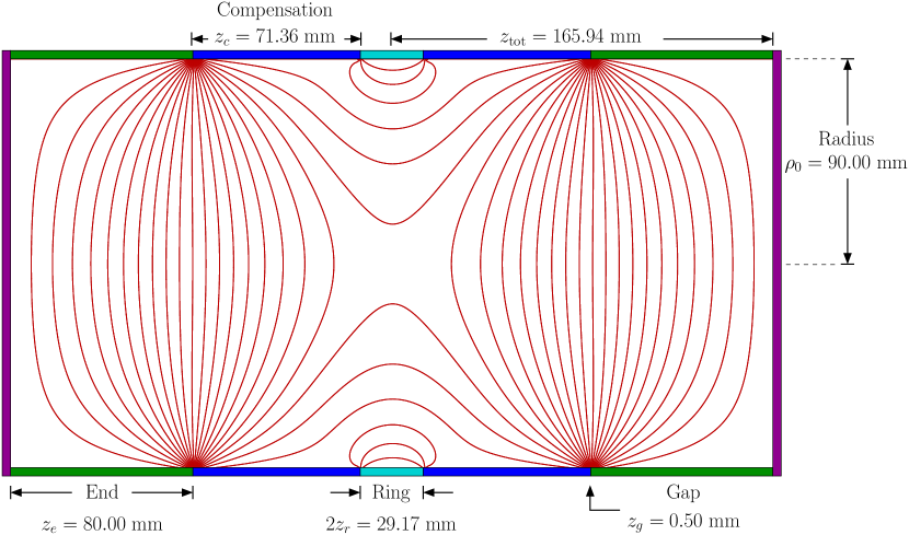
Figure 3: The optimized trap geometry with SIMION generated electric fields lines overlayed.

4 Simulation

The analytic solution for the proposed geometry was verified using SIMION [18], an electric field and ion trajectory simulation program, in order to confirm the validity of the calculations. The results from SIMION are listed in Table 2 (along with the analytic solutions from §3), and the resulting equipotential lines have been overlayed on the geometry cross section presented in Fig. 3. The values output by SIMION agree with the analytic solutions for each $C_{k}$ to a few parts in $10^{-3}$. The discrepancies between the analytic and simulated values can be accounted for by the inherent pixelation of the geometry as represented in SIMION and processing constraints, which have both been minimized as far as allowed by RAM and available computing time. Specifically, the optimized geometry has been represented in the simulation to the nearest $0.01$ mm, and the voltages have been defined to $1\times 10^{-5}$ V.

$C_{i}$	TAMU	TAMU	TITAN	LEBIT
	Analytic	Simulated	Analytic	Simulated
$C_{0}$	$-5\text{\times}{10}^{-1}$	$-5\text{\times}{10}^{-1}$	-	$8\text{\times}{10}^{-1}$
$C_{2}$	$5\text{\times}{10}^{-1}$	$6\text{\times}{10}^{-1}$	-	$1$
$C_{4}$	$-7\text{\times}{10}^{-6}$	$9\text{\times}{10}^{-4}$	$-7\text{\times}{10}^{-6}$	$2\text{\times}{10}^{-3}$
$C_{6}$	$6\text{\times}{10}^{-6}$	$-3\text{\times}{10}^{-3}$	$5\text{\times}{10}^{-5}$	$-4\text{\times}{10}^{-3}$
$C_{8}$	$-4\text{\times}{10}^{-2}$	$-4\text{\times}{10}^{-2}$	-	$3\text{\times}{10}^{-3}$

Table 2: Expansion coefficients are compared for the optimized TAMUTRAP measurement trap when tuned (analytic and simulated) and two other existing Penning traps: TITAN (calculated analytically as in Ref. [19]), and LEBIT (simulated using SIMION as in Ref. [20]).

5 Comparison to Existing Traps

The defining features of the TAMUTRAP geometry described here are the unique inner radius (90 mm), the small $\mathrm{length}/\mathrm{radius}$ ratio ($l/r_{0}=3.72$), and the consideration made for detectors (short endcap electrodes). This new $l/r_{0}$ ratio is what allows TAMUTRAP to exhibit such an unprecedented radial size when compared to other cylindrical Penning traps, while still measuring only 335 mm in overall length. The optimized ISOLTRAP geometry, for example, has an $l/r_{0}=11.75$ [21], and would therefore require over 1 m in length in order to maintain geometrical proportions (and, therefore, electric field shape) with a 90 mm inner radius. The compact geometry employed by TAMUTRAP allows for a structure with a very large radius to easily fit within the 1-m long bore of the 7T 210 ASR magnet. At the same time, the new analytic solution described in §2.3 retains the good quadrupole nature of the electric field displayed by other prominent Penning traps, which is required for other experiments such as precision mass measurements.

Table 2 compares the analytic and simulated electric field expansion coefficients of TAMUTRAP to an analytic solution reported by LEBIT [20], and a simulated solution reported by TITAN [19]. The suppression of the anharmonic terms in the electric field generated by the geometry for the TAMUTRAP measurement Penning trap is comparable to that presented by these two prominent mass-measurement facilities, for which a very well-tuned harmonic electric field is critical [22]. With respect to the inherent field shape, the TAMUTRAP geometry should therefore be suitable for such precision mass measurements; however, it remains to be seen what affects the unprecedented electrode size and trapping volume necessitated by the primary program of performing $\beta-\nu$ correlation measurements will have on the specific procedures required in these studies. In particular, due to the enlarged geometry, the uniformity of the applied potentials across the electrodes is likely to be worse at TAMUTRAP than at existing facilities that employ smaller electrodes. It remains to be seen, however, whether or not these effects will ultimately limit mass resolution. In either case, they will not have a significant effect on the main program where the harmonic potential is not as stringent.

6 Conclusion

A novel, large-bore cylindrical Penning trap with a new $\mathrm{length}/\mathrm{radius}$ ratio in the electrode structure has been described. The design work has been performed with the initial research program of measuring correlation parameters for $T=2$ superallowed $\beta$-delayed proton emitters in mind; however, careful attention has also been paid to creating a facility with maximum suitability for a wide range of possible future nuclear physics experiments. In particular, a line of sight to the trap center, an open geometry, and a well characterized quadrupole electric field are predicted with the proposed design. The analytic solutions to the electric field were checked against simulation, and match to high precision. These values, which are comparable to those presented by existing mass measurement facilities, suggest that TAMUTRAP should be capable of performing mass measurements in addition to its primary program. The aforementioned features, in conjunction with the unprecedented 90 mm free trap radius, will make the TAMUTRAP facility a unique tool for future nuclear physics research.

7 Acknowledgments

The authors would like to thank Guy Savard, Jason Clark, and Jens Dilling for fruitful discussions and advice. This work was supported by the U.S. Department of Energy under Grant Numbers ER41747 and ER40773.

References

- [1] N. Severijns, O. Naviliat-Cuncic, Annu. Rev. Nucl. Part. Sci. 61 (2011) 23–46.
- [2] N. Severijns, M. Beck, O. Naviliat-Cuncic, Rev. Mod. Phys. 78 (2006) 991–1040.
- [3] J. A. Behr, G. Gwinner, J. Phys. G: Nucl. Part. Phys. 36 (3) (2009) 033101.
- [4] I. Towner, J. Hardy, Report on Progress in Physics 73 (4) (2010) 046301.
- [5] N. Severijns, M. Tandecki, T. Phalet, I. Towner, Phys. Rev. C: Nucl. Phys. 78 (2002) 055501.
- [6] E. Adelberger, et al., Phys. Rev. Lett. 83 (7) (1999) 1299–1302.
- [7] J. Jackson, S. Treiman, H. Wyld, Nucl. Phys. 4 (1957) 206–212.
- [8] K. Blaum, Physics Reports 425 (1) (2006) 1–78.
- [9] M. Amoretti, et al., Nature 419 (6906) (2002) 456–9.
- [10] V. Y. Kozlov, et al., Hyperfine Interact. 175 (2006) 15–22.
- [11] M. Mehlman, D. Melconian, P. D. Shidling, arXiv:1208.4078 (Aug. 2012).
- [12] Agilent Technologies, http://www.agilent.com (Aug. 2012).
- [13] C. Roux, et al., arXiv:1110.2920v1 (Oct. 2011).
- [14] D. Beck, et al., Nucl. Instrum. Methods Phys. Res., Sect. B 126 (96) (1997) 378–382.
- [15] G. Gabrielse, L. Haarsma, S. L. Rolston, J. Mass Spectrom. 88 (1989) 319–332.
- [16] Wolfram Research, http://www.wolfram.com (Aug. 2012).
- [17] G. Gabrielse, Phys. Rev. A: At., Mol., Opt. Phys. 27 (5) (1983) 2277.
- [18] Scientific Instrument Services, Inc., http://www.simion.com (Aug. 2012).
- [19] M. Brodeur, Ph.D. thesis, University of British Columbia (2010).
- [20] R. Ringle, et al., Nucl. Instrum. Methods Phys. Res., Sect. A 3 (604) (2009) 536–547.
- [21] H. Raimbault-Hartmann, et al., Nucl. Instrum. Methods Phys. Res., Sect. B 126 (1-4) (1997) 378–382.
- [22] G. Gabrielse, Int. J. Mass Spectrom. 279 (2-3) (2009) 107–112.