Extragalactic number counts at 100 $\mu$m, free from cosmic variance

Abstract

We use data from the DEBRIS survey, taken at 100 $\mu$m with the PACS instrument on board the Herschel Space Observatory, to make a cosmic variance-independent measurement of the extragalactic number counts. These data consist of 323 small area mapping observations performed uniformly across the sky, and thus represent a sparse sampling of the astronomical sky with an effective coverage of $\sim$2.5 deg².

We find our cosmic variance independent analysis to be consistent with previous counts measurements made using relatively small area surveys. Furthermore, we find no statistically significant cosmic variance on any scale within the errors of our data. Finally, we interpret these results to estimate the probability of galaxy source confusion in the study of debris discs.

1 Introduction

One of the most fundamental measurements that can be made from extragalactic survey data is that of source number counts. In most cases a balance between survey area and depth must be struck, typically resulting in a small number of relatively deep compact fields being observed alongside some wider shallow imaging. For example, the largest area surveyed using Herschel (Pilbratt et al., 2010) was the Astrophysical Terahertz Large Area Survey (H-ATLAS; Eales et al., 2010), which covers 550 deg² but still constitutes only 1.3 per cent of the entire sky. In addition, the H-ATLAS observations are relatively shallow, with deeper surveys covering increasingly smaller areas (e.g. Elbaz et al., 2011). Consequently almost all source count measurements are potentially subject to cosmic variance: the statistical uncertainty inherent when inferring results based on data from a finite sub-region or sub-regions of the sky. Only by observing the entire sky can region-to-region fluctuations be averaged out entirely, giving a measurement truly free from cosmic variance.

In this letter we use multiple small-field observations ($\sim$28 arcmin² each) distributed randomly across the entire sky to obtain a cosmic variance independent assessment of the extragalactic source number counts, and characterise the cosmic variance on a wide range of angular scales. This is achieved by treating each field as representative of the larger region which it inhabits. By calculating the source counts for all of these fields at once, we can obtain a measurement which is representative of the entire sky, in which cosmic variance is dramatically reduced compared to contiguous area surveys of a similar size. By producing source counts from various sub-combinations of these fields, we can also estimate the cosmic variance – quantitatively – as a function of angular scale, thereby determining the scale at which a survey can be regarded as effectively free from cosmic variance.

For this analysis we use the 100-$\mu$m data from the Disc Emission via a Bias-free Reconnaissance in the Infrared/Submillimetre survey (DEBRIS; Matthews et al., in preparation), obtained with the Photoconductor Array Camera and Spectrometer instrument (PACS – Poglitsch et al., 2010) on board Herschel. We do not include an analysis of the 160-$\mu$m DEBRIS data, obtained at the same time as the 100-$\mu$m data, as their quality across the fully mapped area was insufficient to achieve a useful measurement of the source counts.

This analysis is not intended to supersede the results in this band from the PACS Extragalactic Probe (PEP – Lutz et al., 2011) presented by Berta et al. (2010), who use significantly deeper observations, or the H-ATLAS results given by Rigby et al. (2011) and Ibar et al. (in preparation), who use a significantly larger total area. Instead this analysis focuses on the comparison of these results with those obtained from our cosmic variance independent measurement of the source counts. Various clustering analyses have already been performed at Herschel wavelengths (e.g. Cooray et al., 2010; Maddox et al., 2010; Magliocchetti et al., 2011), however, these have all been restricted to relatively small scales, with the largest clustering analysis at 100 $\mu$m being at angular scales $\leq 6$ arcmin. Consequently we aim to provide a complementary analysis, focusing on much larger angular scales.

In § 2 we describe the data from which we obtain our source counts, along with our reduction method. § 3 contains a description of our source extraction method, and the simulations we performed to quantify completeness. Our number counts and measurements of cosmic variance as a function of angular scale are given in § 4. These results are then interpreted to assess the impact of background source confusion on general debris disc surveys in § 5. Finally, our conclusions are given in § 6.

2 The data

The DEBRIS survey is a Herschel Open Time Key Programme whose primary science goal is to discover and study debris discs around nearby stars (Matthews et al., in preparation). The target list is generally unbiased, with sources only being excluded if the cirrus confusion noise level at 100 $\mu$m was predicted to be greater than 1.2 mJy for a point source at the time of survey design. The target selection was taken from the Unbiased Nearby Star catalogue (Phillips et al., 2010) with sources being selected sequentially in order of distance from the Sun. With the exception of regions close to the Galactic plane where cirrus confusion is high, the observed fields are distributed uniformly on the sky, with no particular preference in any one direction. The flux limited observing strategy employed by the DEBRIS team also ensures that each region is observed to the same depth, thereby providing a uniform data set.

In this work we search for chance detections of extragalactic sources in the extended imaging around 323 debris disc target fields. The observations were made using the PACS ‘mini-scan map’ observing mode, which provides maps with an area of approximately 3.5 arcmin $\times$ 8 arcmin, giving a total survey area of approximately 2.5 deg². The telescope scanning rate was 20 arcsec s^-1, and the full width half maximum of the resultant 100-$\mu$m beam was 7 arcsec. This observing mode was designed to observe compact and point-like sources, with the majority of the integration time concentrated in the centre of the map.

The maps were reduced using the Herschel Interactive Pipeline Environment (HIPE; Ott, 2010) version 7.0. The standard processing steps were followed and maps were made using the ‘photProject’ task. The data were high-pass filtered using a filter scale of 16 frames, equivalent to 66 arcsec., to suppress $1/f$ noise. The final maps have a 1-$\sigma$ noise level of $\sim$2.0 mJy beam^-1 in the central region.

3 Source catalogue and simulations

Before finding and extracting sources we adjusted the maps to remove any pixels whose integration time was below 25 per cent of the peak map coverage. This was done to remove the noisy edge regions which would confuse a source-extraction algorithm. A circular mask with a radius of 45 arcsec was also applied at the map centre to blank out the original target star coordinates for each field.

We identified sources in the maps using the source-extraction software, SExtractor (Bertin & Arnouts, 1996), and measured the flux density using aperture photometry. An aperture radius of 20 arcsec was used for all sources. Custom aperture corrections were derived for this dataset with reference to the aperture corrections provided by the PACS instrument team. These custom corrections were applied to each measured source to obtain a final flux density measurement.

The fragmented nature of this survey and the highly variable, irregularly shaped coverage within individual maps means it is difficult to determine an accurate survey area and general noise level for this work. To overcome this issue we chose to adopt a reference effective area with a regular shape for each field. The reference area is required to be larger than the range of the measured data and in practice this was simply taken as the total area of the image, including all regions for which no data were obtained. A completeness correction could then be determined based on simulations performed within this reference area. As the reference area is required to be sufficiently large to enable all position angles of the rectangular map, a significant portion of the reference area will always contain no data, meaning that the maximum completeness possible is $\sim 20$ per cent.

To obtain the completeness correction for these data we placed ten simulated point sources of a given flux density randomly into each map. We used observations of Arcturus (observation IDs 1342188248 and 1342188249) – obtained in the same observing configuration as our data – as our point source model. This model was scaled in order to return the expected flux density following application of the appropriate aperture correction. No more than ten sources were input to a single map to avoid increasing the source density to a point wherein the simulated sources might blend and represent an increase in confusion noise). These simulated sources were extracted using the same method as for our original catalogue. The number of simulated sources detected was then obtained by differencing histograms constructed from the original and simulated source catalogues. The resultant histogram showed a Gaussian distribution of sources centred at the flux density of the input (simulated) source. A Gaussian fit was made to this histogram and the number of sources measured was compared to the number of simulated sources to obtain the completeness at this flux density. The fitted width of the Gaussian was also used as a measure of the uncertainty in flux-density measurement for all measured sources. This process was repeated for a range of flux densities to find the completeness correction across the flux densities measured in our original catalogue. The entire simulation process was repeated five times to reduce the uncertainty in the derived correction.

The completeness correction is a statistical result and is only valid when working with the entire survey dataset and the adopted reference map areas. It is not applicable to specific individual regions of real data within any given map. The final DEBRIS galaxy source catalogue consists of 540 sources with a detection significance of $\geq 3\sigma$ and a typical 1-$\sigma$ uncertainty of $\sim 3.0$ mJy. The typical completeness for this catalogue is 14 per cent, which equates to $\sim$65 per cent within the regions of the reference area (described above) in which data exist. The large range of integration times within the map means that completeness levels near 100 per cent could only be achieved for the extremely rare, bright sources.

4 Number counts and cosmic variance

4.1 Number counts

The measured galaxy number counts at 100 $\mu$m, normalised to the Euclidean slope, are given in Table 1 and plotted in Figure 1. The counts obtained at the same wavelength from the PEP (Berta et al., 2010) and H-ATLAS (Rigby et al., 2011) surveys are also given, for comparison, with the three PEP counts being obtained from 2-deg², 450-arcmin² and 140-arcmin² fields for the Cosmic Evolution Survey (COSMOS – Scoville et al., 2007), Lockman Hole and Great Observatories Origins Deep Survey (GOODS-N – Giavalisco et al., 2004) fields, respectively, and the H-ATLAS counts from the 14-deg² science demonstration field. Poisson noise provides the dominant uncertainty in the DEBRIS number counts, with the Eddington bias uncertainty ranging from $\sim$90 to $\sim$50 per cent of the corresponding Poisson noise level from low to high flux densities across the plotted range. The errors quoted are the quadrature sum of these two sources of error.

Table 1: Measured extragalactic number counts, normalised to the Euclidean slope at 100 $\mu$m

Flux density	Number counts	1-$\sigma$ error
(mJy)	($\times 10^{3}$ mJy1.5deg-2)	($\times 10^{3}$ mJy1.5deg-2)
13.7	77.2	6.8
19.0	63.9	7.9
26.3	61.9	9.2
36.5	54.6	10.1
50.7	36.4	9.8
70.3	48.6	14.1
97.4	40.7	14.6

Our number counts are in good agreement with those published by the PEP and H-ATLAS teams, indicating that the results from these individual fields are genuinely representative of the larger-scale galaxy number counts within the given uncertainties of the relative samples.

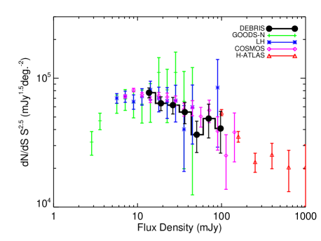
Figure 1: Galaxy source counts at 100 $\mu$m, normalised to the Euclidean slope. Source counts in various well-known survey fields from the PEP (Berta et al., 2010) and H-ATLAS (Rigby et al., 2011) surveys are overlaid for comparison.

4.2 Cosmic variance

To measure cosmic variance on various angular scales we began with the null hypothesis that there was zero cosmic variance on all scales ($\sigma^{2}=0$). This hypothesis was then tested using the formalism set out by Efstathiou et al. (1990). The sky was split into circular cells of equal angular area, $A$, and galaxy number counts, $N$, were obtained for each cell. The cell-to-cell variations were then compared with what would be expected from Poissonian statistics using Equation 9 of Efstathiou et al. (1990),

$$\sigma^{2}=\frac{\sum_{j}(N_{j}-A_{j}\sum_{k}N_{k}/\sum_{k}A_{k})^{2}-(1-\sum_{k}A_{k}^{2}/(\sum_{k}A_{k})^{2})\sum_{j}N_{j}}{(\sum_{j}N_{j}/\sum_{j}A_{j})^{2}[\sum_{k}A_{k}^{2}-2\sum_{k}A_{k}^{3}/\sum_{k}A_{k}+(\sum_{k}A_{k}^{2})^{2}/(\sum_{k}A_{k})^{2}]}.$$ (1)

This generalised equation allows for incomplete cell sampling and is therefore appropriate for the DEBRIS sample (see Efstathiou et al. for details). The uncertainty in this measurement ($\Delta(\sigma^{2})$) was quantified using Equation 5 of Efstathiou et al. (1990). This method was also implemented by Austermann et al. (2010) to assess the level of cosmic variance in four fields imaged with the AzTEC camera at 1.1 mm.

Cells with an angular area equal to that of one DEBRIS map up to 2$\pi$ steradians were tested. The measured variance from each cell size is shown in Figure 2. The measured variances have a median value of $1.2\times 10^{-2}$, in keeping with those reported by Austermann et al. (2010) as well as the model of Moster et al. (2011), within the stated errors. However, in all cases the signal-to-noise ratio ($\sigma^{2}/\Delta(\sigma^{2})$) is less than 3. This indicates that these measurements do not represent a statistically significant detection of a non-zero cosmic variance on scales down to the size of one DEBRIS map.

Figure 2: Measured cell variance (top) and upper limits (bottom) as a function of cell radius. Note that negative $\sigma^{2}$ indicates that the measured variance is less than that expected from Poisson statistics.

Although the non-uniformity and sparse sampling of the DEBRIS data makes it difficult to calculate the angular correlation function for direct comparison with the results of Cooray et al. (2010), Maddox et al. (2010) and Magliocchetti et al. (2011), it is still possible to compare their results with those from this analysis. All three prior publications show a decrease in clustering (i.e. variance) with increasing angular scale. The upper limits we obtain show a similar trend, albeit with very low statistical significance.

Cooray et al. (2010), Maddox et al. (2010) and Magliocchetti et al. (2011) also find increased clustering with higher redshift galaxy populations. Therefore our non-detection of cosmic variance at 100 $\mu$m, which is typically dominated by low redshift ($z\leq 1$) galaxies, is in keeping with these previous results.

The failure to detect cosmic variance in this work could be thought to be, in part, a result of the DEBRIS survey depth. Deeper observations would probe higher-redshift galaxy populations, too faint to detect in the current data. With deeper maps we would therefore expect to observe the same level of clustering at 100 $\mu$m as Cooray et al. (2010) and Maddox et al. (2010) find at 350 and 500 $\mu$m. However, these deeper data would also contain additional faint, low-redshift galaxies with a similarly uniform distribution to the population of nearby galaxies currently observed, thereby diluting the clustering signature of these additional high-redshift sources. In addition, if we assume that the clustering measured at 350 $\mu$m is dominated by galaxies close to the 3-$\sigma$ confusion limit and at $z\sim 2.3$ (Cooray et al., 2010) then the required 1-$\sigma$ survey limit to detect these sources at 100 $\mu$m would be $\sim$0.2 mJy, only slightly higher than the 100-$\mu$m confusion limit. Given these two factors, we conclude that our results are valid for all 100-$\mu$m survey depths down to the limiting survey area of one DEBRIS map, given a comparable confusion noise limit. Therefore, a survey of $\sim$28 arcmin² would be expected to have $\sigma^{2}\leq 0.2$.

5 Relevance to debris discs

Debris discs are most commonly identified by an infrared excess above the predicted photospheric level. It can be extremely difficult to determine accurately whether a measured excess is due to a debris disc or merely a chance alignment with a background galaxy. Some features originally attributed to debris discs have subsequently been found to be background objects, e.g. Greaves et al. (2005); Regibo et al. (2012). Confusion is particularly problematic in statistical studies of debris discs. We expect cases of background contamination will be more likely when analysing many tens of discs, as is the case with the DEBRIS survey. It is therefore helpful to also interpret the results of this analysis in terms of its relevance to debris disc studies.

In order to account for confusion, an accurate estimate of the probability of a background source being present within a given radius of a star is essential. This study has shown that data from DEBRIS observations, typical of almost all debris disc observations made with Herschel, are consistent with data from surveys of typical extragalactic fields. We have also shown that, to within the limits of these data, there is no significant cosmic variance at 100 $\mu$m. Consequently, it is reasonable to make use of the results from deep extragalactic surveys and apply their statistics directly to debris disc observations. For the purposes of estimating background source confusion, we make the assumption that the invariance of the 100-$\mu$m counts can be extended to the other two PACS wavelength bands.

Using the raw measured differential counts of Berta et al. (2011), we estimated the number of sources that could potentially explain an excess at a given flux density. To ensure all potential sources were included, the number counts were weighted by a Gaussian probability density function with a 1-$\sigma$ width equal to the uncertainty of the original measurement. This provides a measurement that includes a contribution due to Eddington bias. We calculated the number of galaxies for all flux density bins given by Berta et al. (2011) over a wide range of $\sigma$ values, then fitted a two-dimensional polynomial to the output grid. Magliocchetti et al. (2011) do find clustering in these data on small scales, but the level of clustering is extremely low, and none of the measurements is statistically significant ($<3\sigma$ in all cases). As a result, we regard these data to be unclustered for the purposes described in this section. The number of galaxies per square degree, $N$, at a given flux density, $S_{\lambda}$, and measurement uncertainty, $\sigma$, can thus be estimated directly from the resultant polynomial fit,

$$\log_{10}N=\sum\limits_{i,j=0}^{2}k(\lambda)_{i,j}\log_{10}\sigma^{i}\log_{10}S_{\lambda}^{j},$$ (2)

where $k(\lambda)_{i,j}$ is the matrix of polynomial coefficients derived for the fit. These matrices for flux densities measured in mJy for each wavelength are,

$$k(70\,\mu\rm{m})=\begin{bmatrix}3.34&-0.770&-0.470\\ -2.45\times 10^{-4}&-2.23\times 10^{-3}&5.23\times 10^{-3}\\ 4.41\times 10^{-6}&-2.31\times 10^{-6}&-1.89\times 10^{-5}\end{bmatrix},$$

$$k(100\,\mu\rm{m})=\begin{bmatrix}3.84&-1.10&-0.181\\ -0.0108&0.0340&-0.0180\\ 7.94\times 10^{-5}&-2.58\times 10^{-4}&1.44\times 10^{-4}\end{bmatrix},$$

$$k(160\,\mu\rm{m})=\begin{bmatrix}4.12&-1.04&-0.142\\ -0.0208&0.0455&-0.0210\\ 1.00\times 10^{-4}&-2.35\times 10^{-4}&1.17\times 10^{-4}\end{bmatrix}.$$

Therefore, given an expected background source number density $N(S_{\lambda},\sigma)$, the Poisson probability of $n$ sources existing within radius $r$ (in arcsec) is given by,

$$P(n,<r,N)=\exp\left(-\frac{N\pi r^{2}}{3600^{2}}\right)\frac{(N\pi r^{2}/3600^{2})^{n}}{n!}.$$ (3)

Using this formalism it is possible to calculate the probability of a background source being present in PACS observations of debris discs with an excess ranging from $\sim$2–140 mJy. Table 2 gives the probability of a source being present within a beam half-width half-maximum radius of a given source location, for a range of typical levels of measured excess flux density. In all cases the source is assumed to have been detected at the 3-$\sigma$ level. These values have been calculated using Equation 2 and have been found to have a 1-$\sigma$ variation of 2.6$\times 10^{-3}$ with respect to probabilities calculated directly from the original data.

These results are suitable when estimating the confusion of an individual source with a clearly measured excess. However, when working with a survey consisting of many observations, looking at the probability of confusion at a specific flux density is less useful than asking the question what fraction of sources are likely to be confused by any number of background sources?

Table 2: Probability, calculated using Equation 2, of one background source existing within a beam half-width half-maximum radius of the measured source loaction for a range of measured exccess flux densities. In all cases the excess emission is assumed to be detected at the 3-$\sigma$ level.

$S_{\lambda}$ (mJy)	P${}_{70\mu\rm{m}}\times 10^{-4}$	P${}_{100\mu\rm{m}}\times 10^{-4}$	P${}_{160\mu\rm{m}}\times 10^{-4}$
3	11	59	300
4	7.9	41	220
6	4.5	24	130
10	2.0	12	71
20	0.6	4.2	28
100		0.12	1.1

The cumulative extragalactic number counts can be used to estimate the probability of confusion, by one or more background sources, by integrating the counts from the survey limiting flux density, $S_{\rm{lim}}$, to the upper limit of the data. This number of galaxies, $N_{\rm c}$, can then be input to the cumulative Poisson probability equation,

$$P_{\rm c}(n,<r,N_{\rm c})=\exp\left(-\frac{N_{\rm c}\pi r^{2}}{3600^{2}}\right)\sum\limits_{i}^{n}\frac{(N_{\rm c}\pi r^{2}/3600^{2})^{i}}{n!},$$ (4)

where $P_{\rm c}$ is the probability of confusion with $n$ or more background sources within a given radius $r$.

Using the raw cumulative number counts, however, does not take account of Eddington bias. Due to the steep slope of the counts a larger number of sources will be boosted above $S_{\rm{lim}}$ than will be boosted down, making this ‘naïve’ measurement of $N$ an underestimate. To assess the significance of Eddington bias in this case we used the cumulative number counts from Berta et al. (2011) and performed a Monte-Carlo simulation. Simulations were performed for a range of limiting survey flux density and region radii, and the output is given in Figure 3.

Figure 3: Probability of confusion by one or more background sources as a function of survey limiting flux density calculated via the Monte-Carlo method (symbols) and the naïve method (dashed line). Polynomial fits made in log-log space to the Monte-Carlo points are plotted as solid lines, with the fitted equations given in the top right of each panel. In all cases the limiting flux density is assumed to be the 3-$\sigma$ limit for the given survey. Results are shown for confusion within various radii of a given source location.

Results from the naïve and Monte-Carlo methods are in good agreement for faint survey limits, but begin to diverge at limits greater than $\sim$10 mJy, with the naïve method systematically underestimating the confusion. In these bright survey limit cases, the increased measurement uncertainty results in a higher contribution from Eddington bias and thus an underestimate in the naïve estimate of $N_{\rm c}$. Note that the increase in the measurement uncertainty is a result of our assumption that the $S_{\rm{lim}}$ is a 3-$\sigma$ limit. For higher survey thresholds, e.g. 5-$\sigma$, the deviation between the two methods would begin at higher flux densities.

These results are applicable for surveys without a single, limiting flux density. In this case the probability of confusion for each observation, given its own limiting flux density, can be estimated and combined for all observations in the standard way to estimate the probability of source confusion.

6 Conclusions

We find our galaxy number counts – based on observations that sparsely sample the entire sky in a uniform manner – to be in agreement with previous studies whose results are derived from relatively small-area surveys. We also measure no statistically significant non-zero cosmic variance on scales of $\sim$28 arcmin² (the scale of a DEBRIS map) up to 2$\pi$ steradians, providing only upper limits. We conclude that traditional, relatively small-area surveys, such as those undertaken by the PEP and H-ATLAS teams, are in general sufficiently representative to measure and characterise the extragalactic number counts in a universal context.

References

- Austermann et al. (2010) Austermann J. E., et al., 2010, MNRAS, 401, 160
- Berta et al. (2010) Berta S., et al., 2010, A&A, 518, L30
- Berta et al. (2011) Berta, S., Magnelli, B., Nordon, R., et al. 2011, A&A, 532, A49
- Bertin & Arnouts (1996) Bertin E., Arnouts S., 1996, A&AS, 117, 393
- Cooray et al. (2010) Cooray, A., Amblard, A., Wang, L., et al. 2010, A&A, 518, L22
- Eales et al. (2010) Eales S., et al., 2010, PASP, 122, 499
- Efstathiou et al. (1990) Efstathiou G., Kaiser N., Saunders W., Lawrence A., Rowan-Robinson M., Ellis R. S., Frenk C. S., 1990, MNRAS, 247, 10P
- Elbaz et al. (2011) Elbaz D., et al., 2011, A&A, 533, A119
- Giavalisco et al. (2004) Giavalisco M., et al., 2004, ApJ, 600, L93
- Greaves et al. (2005) Greaves, J. S., Holland, W. S., Wyatt, M. C., et al. 2005, ApJL, 619, L187
- Lutz et al. (2011) Lutz D., et al., 2011, A&A, 532, A90
- Moster et al. (2011) Moster B. P., Somerville R. S., Newman J. A., Rix H.-W., 2011, ApJ, 731, 113
- Maddox et al. (2010) Maddox S. J., et al., 2010, A&A, 518, L11
- Magliocchetti et al. (2011) Magliocchetti M., et al., 2011, MNRAS, 416, 1105
- Ott (2010) Ott S., 2010, ASPC, 434, 139
- Phillips et al. (2010) Phillips N. M., Greaves J. S., Dent W. R. F., Matthews B. C., Holland W. S., Wyatt M. C., Sibthorpe B., 2010, MNRAS, 403, 1089
- Pilbratt et al. (2010) Pilbratt G. L., et al., 2010, A&A, 518, L1
- Poglitsch et al. (2010) Poglitsch A., et al., 2010, A&A, 518, L2
- Rigby et al. (2011) Rigby E. E., et al., 2011, MNRAS, 415, 2336
- Regibo et al. (2012) Regibo, S., Vandenbussche, B., Waelkens, C., et al. 2012, A&A, 541, A3
- Scoville et al. (2007) Scoville N., et al., 2007, ApJS, 172, 1