Kondo effect on the surface of 3D topological insulators:
Signatures in scanning tunneling spectroscopy

Abstract

We investigate the scattering off dilute magnetic impurities placed on the surface of three-dimensional topological insulators. In the low-temperature limit, the impurity moments are Kondo-screened by the surface-state electrons, despite their exotic locking of spin and momentum. We determine signatures of the Kondo effect appearing in quasiparticle interference (QPI) patterns as recorded by scanning tunneling spectroscopy, taking into account the full energy dependence of the T matrix as well as the hexagonal warping of the surface Dirac cones. We identify a universal energy dependence of the QPI signal at low scanning energies as the fingerprint of Kondo physics, markedly different from the signal due to non-magnetic or static magnetic impurities. Finally, we discuss our results in the context of recent experimental data.

I Introduction

Topological insulators (TIs) in both two and three spatial dimensions constitute an active topic of current condensed matter research.Kane and Mele (2005); Bernevig et al. (2006); König et al. (2007); Fu et al. (2007); Moore and Balents (2007); Qi et al. (2008); Roy (2009) The non-trivial bulk band topology of three-dimensional (3D) strong topological insulators causes the crossing of surface states at time-reversal invariant points in the surface Brillouin zone and gives rise to a two-dimensional surface metal. In the vicinity of such crossing points, the effective surface theory takes the form of a Dirac equation of massless fermions, where spin and momentum are locked together.

A fundamental property of this “helical” surface metal is a suppression of backscattering: Electrons with opposite momenta have orthogonal spin projections, such that impurity scattering $\vec{k}\leftrightarrow-\vec{k}$ is impossible without a spin flip. As a result, the metallic state is protected from the influence of non-magnetic disorder, and weak localization is replaced by weak antilocalization.Bardarson et al. (2007); Nomura et al. (2007) This scenario of forbidden backscattering has been tested in recent experimentsRoushan et al. (2009); Alpichshev et al. (2010); Zhang et al. (2009); Okada et al. (2011); Hsieh et al. (2008); Xia et al. (2009) utilizing powerful Fourier-transform scanning tunneling spectroscopyCrommie et al. (1993); Lee et al. (2009a) (FTSTS). In this technique, energy-dependent spatial variations of the local density of states (LDOS) are analyzed in terms of quasiparticle interference (QPI), i.e., quasiparticle scattering processes due to impurities. The QPI results obtained on 3d TIs such as Bi_1-xSb_x and Bi₂Te₃ were found to be consistent with a heuristic picture of electron scattering in a helical liquid, with backscattering being suppressed.

These results prompt the question as to how scattering from magnetic impurities on the surface of TIs is manifest in observables such as the QPI patterns obtained by FTSTS. In fact, recent experimentsOkada et al. (2011) on Bi₂Te₃ doped with dilute magnetic Fe atoms purport to demonstrate from the QPI pattern signatures of time-reversal symmetry breaking. However, one must be careful to distinguish a fluctuating magnetic moment from one which is static on the large timescale of the STS experiment. The latter situation implies magnetic long-range order, whose existence requires a sufficient density of magnetic moments and low temperature. Then, every impurity moment is polarized, and time-reversal symmetry is broken.Liu et al. (2009) Interestingly, it has been shown theoretically that such static magnetic impurities do not lead to backscattering being visible in QPI; within lowest-order Born approximation, a static local field is entirely invisible in QPI.Zhou et al. (2009); Guo and Franz (2010)

In this paper, we focus instead on the case of fluctuating magnetic impurities, relevant to the dilute limit. The interaction between the impurity moment and the electrons of the surface metal leads to mutual spin flips, such that backscattering could be allowed although time-reversal symmetry remains unbroken. It is such spin-flip processes which lead to Kondo screening of the impurity moment in standard metals.Hewson (1993) Therefore the key question, also relevant to the experiments of Ref. Okada et al., 2011, pertains to the signatures in QPI of the Kondo interaction between the helical metal and the impurity. To answer this, we solve the problem of a single Kondo impurity on the surface of a 3D TI numerically exactly, and calculate the induced QPI pattern which of course now includes inelastic scattering off the magnetic moment.

Our main findings are as follows. (i) The magnetic impurity is described by a standard SU(2)-symmetric impurity model, despite spin–momentum locking and hexagonal warping effects of the surface states of a real TI. As a result, the impurity moment is always Kondo screened in the low-temperature limit, unless the chemical potential is tuned exactly to the Dirac point. (ii) While scattering off a Kondo impurity does not open new scattering channels in momentum space as compared to a non-magnetic impurity, it leads to a distinct energy dependence of the QPI pattern, which moreover exhibits universal scaling in terms of both scanning energy and temperature. A strong enhancement of the QPI intensity near the Fermi level is therefore a signature of scattering caused by fluctuating magnetic impurities.

The body of the paper is organized as follows. We start by introducing the model and methods in Sec. II. The Kondo effect on the surface of 3D TIs is discussed in Sec. III. Sec. IV is then devoted to the QPI patterns from Kondo impurities, with an emphasis placed on universal features. The QPI signal from non-magnetic impurities is shown for comparison in Appendix B while we briefly discuss a static magnetic impurity in Appendix C. The implications of our results for experimental data are discussed in the concluding section V.

We note that the Kondo effect on the surface of 3D TIs was discussed before in Refs. Zitko, 2010; Tran and Kim, 2010, but without taking into account hexagonal warping and without a discussion of QPI. QPI patterns for surfaces of 3D TIs have been calculated for different types of impurities in Refs. Guo and Franz, 2010; Lee et al., 2009b; Roushan et al., 2009; Okada et al., 2011; Zhou et al., 2009, but no link to Kondo physics was made. Very recently, inelastic scattering from excited states of magnetic impurities was discussed in Ref. tha, , leading to features at elevated-energy in tunneling spectra.

II Model and Methods

II.1 Effective surface metal

Surface states of 3D TIs are described by an effective Dirac theory. However, such a linearized model applies only in the immediate vicinity of the crossing point of the surface bands, while lattice effects must be taken into account at higher energies. For Bi₂Te₃ this results in a breaking of the continuous rotation symmetry around the Dirac point down to $C_{3v}$, leading to so-called hexagonal warping of the iso-energy contours,Fu (2009) as is seen experimentally.Hsieh et al. (2009); Chen et al. (2009); Roushan et al. (2009); Okada et al. (2011)

The free Hamiltonian of the surface metal readsFu (2009); Lee et al. (2009b)

$$H_{0}=\int d^{2}{\bf{k}}\left(\Psi^{\dagger}_{\bf{k}\uparrow},\Psi^{\dagger}_{\bf{k}\downarrow}\right)\hat{\mathcal{H}}_{\bf{k}}\left(\begin{array}[]{c}\Psi^{\phantom{\dagger}}_{{\bf{k}}\uparrow}\\ \Psi^{\phantom{\dagger}}_{{\bf{k}}\downarrow}\end{array}\right)$$ (3)

where

$$\hat{\mathcal{H}}_{\bf{k}}=\hbar v_{F}\left[({\bf{k}}\times\boldsymbol{\sigma})\cdot{\bf{e}}_{z}+A^{2}k^{3}\cos(3\phi_{\bf{k}})\sigma_{z}\right]-\mu\;.$$ (4)

Here $\boldsymbol{\sigma}$ is a vector of the Pauli matrices, $k=|\bf{k}|$ is the magnitude of the momentum vector relative to the Dirac point, and $\phi_{\bf{k}}=\tan^{-1}(k_{y}/k_{x})$ is its azimuthal angle measured with respect to the $\hat{x}$ axis. The $\Gamma$–$K$ direction thus corresponds to $\phi_{\bf{k}}=0$ while $\Gamma$–$M$ corresponds to $\phi_{\bf{k}}=\pi/6$, following Ref. [Lee et al., 2009b]. The cubic term $\propto A^{2}$ accounts for hexagonal warping, and $\mu$ denotes the chemical potential.

The spectrum of the above Hamiltonian (with $\hbar=1$ hereafter) is given by

$$E_{\pm}({\bf{k}})=\pm v_{F}\sqrt{k^{2}+\left[A^{2}k^{3}\cos\left(3\phi_{\bf{k}}\right)\right]^{2}}-\mu\;.$$ (5)

The free Green function, $\hat{G}^{(0)}(\textbf{k},\omega)=[\omega+i0^{+}-\hat{\mathcal{H}}_{\bf{k}}]^{-1}$, takes a diagonal form in the quasiparticle basis, $\hat{\mathcal{G}}^{(0)}_{ab}(\textbf{k},\omega)=\delta_{ab}/[\omega+i0^{+}-E_{a}(\textbf{k})]$, $a,b=\pm$. The density of states (DOS) follows from

$$\rho^{(0)}(\omega)=-\frac{1}{\pi N}\text{Im}~{}\text{Tr}~{}\hat{\mathcal{G}}^{(0)}(\bf{k},\omega),$$ (6)

where the trace accounts for the sum over $\pm$ as well as $\bf{k}$, and $N$ is a suitable normalization factor (equal to the number of $\bf{k}$ points).con $\rho^{(0)}(\omega)$ is linear in $|\omega|$ at low energies around $\omega=-\mu$, characteristic of massless Dirac fermions.

In the following we shall employ parameters $v_{F}/a_{0}=0.73\,$eV ($a_{0}=1$ is a lattice constant acting) as our energy unit, and $A^{2}=2.23$ to make contact with experiments.Okada et al. (2011) For convenience we shall use $v_{F}/a_{0}$ as high-energy cut-off for the conduction band, $\rho^{(0)}(\omega)\equiv\rho^{(0)}(\omega)\theta(v_{F}-|\omega+\mu|)$ – this is mainly needed to generate an input for the numerical treatment of the impurity problem in Sec. III. (For a 3D TI, a natural cutoff is set by the size of the bulk gap.) Generically, the Fermi level is not at the Dirac point; for example, in Ref. Okada et al., 2011 the chemical potential is $\mu/v_{F}=0.137\equiv 100$ meV. Below we consider this case explicitly, and also the special case where $\mu=0$, which is potentially attainable, since surfaces of TIs can be individually gated.

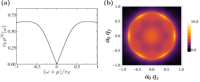
Figure 1: (color online) (a) Density of states, $\rho^{(0)}(\omega)$, for the effective surface theory, Eq. (4) in the absence of impurities, for $A^{2}=2.23$. At energies around $\omega=-\mu$ one obtains linear pseudogap behavior, which is modified at higher energies due to hexagonal warping. (b) QPI pattern $\Delta\rho({\bf{q}},\omega)$ for a TI with $\rho^{(0)}(\omega)$ as in (a), using $T^{0}(\omega)=1$ appropriate for a potential scatterer in Born approximation. Plotted for $\mu/v_{F}=0.137\equiv 100$ meV and scanning energy $\omega=200$ meV.

The local Green function on the surface of the TI has a matrix structure in spin space which turns out to be diagonal:

$$\hat{G}^{(0)}\left(\textbf{r}=0,\omega_{n}\right)=\mathbb{I}f_{\omega_{n},\mu}\;,$$ (7)

in terms of Matsubara frequency $\omega_{n}$. Here

$$f_{\omega_{n},\mu}=\int_{\bf{k}}\frac{i\omega_{n}+\mu}{\left(i\omega_{n}+\mu\right)^{2}-v_{F}^{2}k^{2}-v_{f}^{2}A^{4}k^{6}\cos\left(3\phi_{\bf{k}}\right)^{2}}\;,$$ (8)

where $\int_{\bf{k}}=\int\frac{d^{2}{\bf{k}}}{(2\pi)^{2}}$, such that $\rho^{(0)}(\omega)=-2{\rm Im}\,f_{\omega,\mu}/\pi$. As shown in Appendix A, the off-diagonal elements of $\hat{G}^{(0)}(\textbf{r}=0)$ vanish on angular integration.

II.2 Impurities and QPI

The FTSTS technique exploits scattering of charge carriers from impurities in an otherwise translationally-invariant system.Crommie et al. (1993); Lee et al. (2009a) To this end, a real-space map of the tunneling conductance is recorded at fixed energy. The Fourier transform of this map to momentum space reveals characteristic wavevectors of LDOS inhomogeneities which can be understood as energy-dependent Friedel oscillations (or QPI). In the simplest approximation, these wavevectors correspond to scattering processes of quasiparticles between different points of the dispersion iso-energy contour at the scanning energy.Capriotti et al. (2003)

If scattering centers are dilute, it is sufficient to consider a single impurity. Its effect is described by the T matrix, $\hat{T}_{\textbf{k},\textbf{k}^{\prime}}(\omega)$, such that the full electronic Green function reads

$$\hat{G}(\textbf{k},\textbf{k}^{\prime},\omega) = \hat{G}^{(0)}(\textbf{k},\omega)\delta_{\textbf{k},\textbf{k}^{\prime}}$$ (9)

$$+ \hat{G}^{(0)}(\textbf{k},\omega)\hat{T}_{\textbf{k},\textbf{k}^{\prime}}(\omega)\hat{G}^{(0)}(\textbf{k}^{\prime},\omega)\,,$$

which remains energy-diagonal in equilibrium/linear response. The real-space LDOS is

$$\rho({\bf{r}},\omega)=-\frac{1}{\pi}{\rm{Im}}~{}\int_{\bf q}e^{i{\bf q}\cdot\textbf{r}}~{}{\rm{Tr}}~{}\hat{G}(\textbf{k},{\bf{k}}-{\bf{q}},\omega)\,,$$ (10)

where the trace again accounts for the sum over k as well as the spin components. For isotropic scattering and an inversion-symmetric host, the Fourier transform $\rho({\bf{q}},\omega)$ is real, and its impurity-induced piece is related to the T matrix via

$$\Delta\rho({\bf{q}},\omega)=-\frac{1}{\pi}{\rm{Im}}~{}{\rm{Tr}}~{}\hat{G}^{(0)}({\bf{k}},\omega)\hat{T}_{{\bf{k}},{\bf{k}}-{\bf{q}}}(\omega)\hat{G}^{(0)}({\bf{k}}-{\bf{q}},\omega).$$ (11)

If the T matrix is diagonal in spin space (see below), decomposition using the Pauli matrices gives

$$\hat{T}_{{\bf{k}},{\bf{k}}^{\prime}}(\omega)=T^{0}_{{\bf{k}},{\bf{k}}^{\prime}}(\omega)\mathbb{I}+T^{1}_{{\bf{k}},{\bf{k}}^{\prime}}(\omega)\sigma_{z}\;,$$ (12)

with $T^{0,1}_{{\bf{k}},{\bf{k}}^{\prime}}(\omega)=\left[T_{{\bf{k}},{\bf{k}}^{\prime},\uparrow}(\omega)\pm T_{{\bf{k}},{\bf{k}}^{\prime},\downarrow}(\omega)\right]/2$. For TI surfaces in the absence of hexagonal warping it was shown in Ref. Guo and Franz, 2010 that only the part proportional to $\mathbb{I}$ leads to a modulation of the spin-integrated LDOS in Eqs. (10,11). (The part proportional to $\sigma_{z}$ causes opposite modulations for both spin directions.) Using symmetry properties, we have verified that this still holds for the full model including hexagonal warping: the argument parallels that given in Appendix A.

Specializing further to a point-like impurity with $\hat{T}_{{\bf{k}},{\bf{k}}^{\prime}}(\omega)\equiv\hat{T}(\omega)/N$, we have

$$\Delta\rho({\bf{q}},\omega)=-\frac{1}{\pi}{\rm{Im}}~{}T^{0}(\omega)~{}{\rm{Tr}}~{}\hat{G}^{(0)}({\bf{k}},\omega)\hat{G}^{(0)}({\bf{k}}-{\bf{q}},\omega)$$ (13)

such that the momentum dependence of the QPI signal at fixed $\omega$ is completely determined by $\hat{G}^{(0)}$. A sample QPI image is displayed in Fig. 1 – this is similar to published results.Zhou et al. (2009) One clearly observes a breaking of the circular symmetry due to hexagonal warping of the iso-energy contour at this energy.

As we show below, a (local) Kondo impurity does not modify the overall momentum dependence of the QPI pattern, but will lead to a non-trivial energy dependence.

II.3 Anderson impurity model

To describe a dynamic magnetic scatterer, we consider Anderson’s model for a point-like correlated impurity,Hewson (1993) $H=H_{0}+H_{\text{imp}}+H_{\text{hyb}}$, with

$$\begin{split}H_{\text{imp}}&=\epsilon_{d}(\hat{n}^{d}_{\uparrow}+\hat{n}^{d}_{\downarrow})+U\hat{n}^{d}_{\uparrow}\hat{n}^{d}_{\downarrow}\;,\\ H_{\text{hyb}}&=g\sum_{\sigma}d^{\dagger}_{\sigma}\Psi^{\phantom{\dagger}}_{\sigma}(r=0)+{\text{H.c.}}.\end{split}$$ (14)

Here $\Psi_{\sigma}(r\!=\!0)=\sum_{\textbf{k}}\Psi_{\textbf{k}\sigma}/\sqrt{N}$, $\hat{n}^{d}_{\sigma}=d^{\dagger}_{\sigma}d^{\phantom{\dagger}}_{\sigma}$, and $\epsilon_{d}<0$ and $U>-\epsilon_{d}$ are the local level energy and Coulomb repulsion, respecively.

Considering the spin-momentum locking and the hexagonal warping of the TI surface electrons in $H_{0}$, one might have expected an unconventional impurity problem. However, a standard SU(2) spin-symmetric impurity problem is obtained, with the complexity of the helical surface metal entering only through the unusual DOS, Eq. (6). The derivation of such a pseudogap Anderson (or Kondo) model has been established before for impurities in $d$-wave superconductorsFritz and Vojta (2005) as well as for TIs with a perfect Dirac structure,Zitko (2010); Tran and Kim (2010) and we give here an efficient proof which also covers hexagonal warping. Rather than using a decomposition into angular modes as in Refs. Zitko, 2010; Tran and Kim, 2010, a more direct way is to use the path-integral formulation. Since the conduction-electron bath is Gaussian, we integrate it out exactlyFritz and Vojta (2005) to derive a local retarded impurity problem. The local non-interacting part of the action for the d-levels in Matsubara formalism reads

$$\mathcal{S}_{0}=-T\sum_{\omega_{n}}\overline{{\bf{d}}}^{T}\left[g^{2}\hat{G}^{(0)}\left(\textbf{r}=0,i\omega_{n}\right)-\mathbb{I}(\epsilon_{d}-i\omega_{n})\right]{\bf{d}}\;,$$ (15)

with $\hat{G}^{(0)}\left(\textbf{r}=0,i\omega_{n}\right)$ given in Eq. (7) and ${\bf{d}}=(d_{\uparrow},d_{\downarrow})$. The resulting local model is equivalent to the standard Anderson model because $\hat{G}^{(0)}\left(\textbf{r}=0,i\omega_{n}\right)$ is diagonal. The hybridization function characterizing this impurity problem is

$$\Delta(\omega)=-\text{Im}~{}g^{2}f_{\omega,\mu}=\frac{\pi}{2}g^{2}\rho^{(0)}(\omega)\;.$$ (16)

Importantly, the impurity Green function $\hat{G}^{d}(\omega)$ is diagonal due to the absence of off-diagonal terms in the quadratic action of the d-levels, Eq. (15). In the absence of a magnetic field, we thus have

$$\hat{G}^{d}(\omega)=\frac{1}{\omega+i0^{+}-\epsilon_{d}-g^{2}f_{\omega,\mu}-\Sigma^{d}(\omega)}~{}\mathbb{I}\;.$$ (17)

Here $\Sigma^{d}(\omega)$ is the interaction part of the impurity self-energy. The corresponding T matrix is then $\hat{T}_{\textbf{k},\textbf{k}^{\prime}}(\omega)=g^{2}\hat{G}^{d}(\omega)/N\propto\mathbb{I}$, and one expects a non-trivial response from Anderson-type impurities in QPI according to Eq. (13).

III Kondo effect

The Anderson impurity model, Eq. (14), can describe both the formation and the subsequent screening of local magnetic moments. Charge fluctuations induce two broadened peaks (“Hubbard satellites”) in the impurity spectral function at $\epsilon_{d}$ and $(U+\epsilon_{d})$. The physics at energies smaller than ${\rm min}(-\epsilon_{d},U+\epsilon_{d})$ is dominated by spin-flip processes leading to Kondo screening below a temperature $T_{\rm K}$ – a phenomenon which is sensitive to the conduction-band DOS near the Fermi level.Hewson (1993) Given the unusual DOS of the TI’s surface metal, which vanishes linearly at $\omega=-\mu$, the Kondo effect should be discussed separately in the two cases: (A) the chemical potential is tuned to the Dirac point, $\mu=0$; (B) finite chemical potential, $\mu\neq 0$.

We will obtain numerical results for the Anderson impurity model using Wilson’s numerical renormalization group (NRG) technique.Bulla et al. (2008) In the following, the hybridization function, Eq. (16), is discretized logarithmically using $\Lambda=3$, and $\sim 3000$ states are retained at each step of the iterative diagonalization. The results of $z=3$ interleaved calculationsOliveira and Oliveira (1994) are then combined for optimal results. The full density matrixPeters et al. (2006); Weichselbaum and von Delft (2007) is calculated, and from it the impurity spectral function is determined numericallyWeichselbaum and von Delft (2007) as a full function of energy, $\omega$, at arbitrary temperature, $T$. The real part of $G^{d}$ is obtained using Kramers-Kronig relations. The T matrix and hence QPI can then be calculated via Eq. (13).

We note that the full DOS at the surface of a 3D TI will also have higher-energy contributions from bulk states, not captured by our modelling. Consequently, our calculation cannot establish a quantitative link between the parameters of the Anderson model and $T_{\rm K}$. At present, there is no experimental information available on the actual values of $T_{\rm K}$ for concrete TI materials and impurities. Therefore we choose parameters of Eq. (14) such that $T_{\rm K}$ attains values of order 1 K. For most calculations, we shall employ parameters $U/v_{F}=0.3$, $\epsilon/v_{F}=-0.1$, and $g/v_{F}=0.168$ (chosen to match some elevated-energy features of the data in Ref. Okada et al., 2011), corresponding to a moderately correlated impurity. Results are shown for $T=0$ unless otherwise noted.

III.1 Chemical potential at the Dirac point

For $\mu=0$, the density of states at low energies is $\rho^{(0)}(\omega)\propto|\omega|^{r}$ with $r=1$. The low-energy physics is thus that of the pseudogap Kondo model.Withoff and Fradkin (1990); Gonzalez-Buxton and Ingersent (1998); Bulla et al. (2000); Vojta and Fritz (2004); Fritz and Vojta (2004) For the case of particle–hole symmetry in both the impurity ($\epsilon_{d}=-U/2$) and the bath, screening is absent for all parameters, and the impurity moment remains free down to the lowest energy/temperature scales. In contrast, if particle–hole symmetry is broken, a quantum phase transition occurs, separating the local-moment and Kondo screened phases. However, the latter requires strong particle–hole asymmetry and impurity-host coupling, such that screening is less likely to occur at the Dirac point.

A typical impurity spectral function $A(\omega)=-\text{Im}~{}G_{\sigma}^{d}(\omega)/\pi$ for $\mu=0$ in the local-moment phase at $T=0$ is shown in Fig. 2(a). At high energies ($\omega/v_{F}\approx-0.1$ and $\omega/v_{F}\approx 0.2$) clear signatures of the Hubbard satellites are observed. At low energies (see inset) spectral weight is suppressed due to the pseudogapped free density of states.Bulla et al. (2000); Vojta and Bulla (2002)

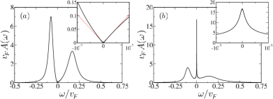
Figure 2: (Color online) Impurity spectral function $v_{F}A(\omega)$ vs energy $\omega/v_{F}$ at $T=0$ for $U/v_{F}=0.3$, $\epsilon/v_{F}=-0.1$, and $g/v_{F}=0.168$. (a) Deep in the local moment phase for $\mu=0$. Inset shows a close-up in the vicinity of the Fermi level, with the linear soft-gap in the free density of states showing up at low energies (red dotted line is $v_{F}A(\omega)\sim|\omega|$). (b) Deep in the Kondo screened phase, $\mu=100$ meV. Inset shows a close-up of the Kondo resonance.

III.2 Chemical potential away from the Dirac point

For finite chemical potential, $\mu\neq 0$, there is a finite density of states at the Fermi level. The impurity is always screened by the Kondo effect on the lowest energy scales (although the Kondo temperature, $T_{\rm K}$, itself might be very small). Screening is reflected in the impurity spectral function by a narrow resonance around the Fermi level. Together with the high-energy Hubbard satellites, this three-peak structure is the classic hallmark of the Kondo effect.

In Fig. 2(b) we plot the spectral function for an impurity with for the same parameters as in panel (a), but with $\mu=100$ meV. The inset shows a close-up of the Kondo resonance, of width $T_{\rm K}\approx 10^{-4}v_{F}\sim 1$ K [we define $T_{\rm K}$ via $A(\omega=T_{\rm K})=\tfrac{1}{2}A(\omega=0)$].

For $\mu$ values closer to the Dirac point, the impurity model will display non-trivial crossover phenomena,Vojta et al. (2010) different from those of the standard Kondo problem,Hewson (1993) due to the non-constant DOS and the proximity to the $\mu=0$ quantum phase transition. Such crossovers can be expected when $\mu\lesssim T_{\rm K}$ and are not present in Fig. 2(b).

IV QPI from dynamic magnetic impurities

We now calculate the QPI pattern, $\Delta\rho({\bf{q}},\omega)$, induced by a dynamic magnetic impurity on the surface of a 3D TI, first for the generic situation of finite chemical potential and then for the special case where the chemical potential is tuned to the Dirac point. We recall that $\Delta\rho({\bf{q}},\omega)$ is real for our case of a single impurity; experiments typically extract its absolute value.

IV.1 Kondo phase

A finite chemical potential implies Kondo screening at lowest temperatures. We divide our analysis into the regimes of elevated and low energies.

IV.1.1 Elevated energies, $\omega\gg T_{\rm K}$

The QPI pattern obtained at high energies 200–360 meV for $\mu=100$ meV is shown in Fig. 3. Upon increasing the scanning energy, the high-intensity peaks move outwards and become more pronounced. This is to be expected from the increasing diameter of the Fermi surface and the increasing importance of hexagonal warping, which is due to the underlying lattice structure and gives rise to the six-fold symmetry. We recall that our modelling neglects bulk bands which will contribute to the signal at energies beyond the bulk gap.Okada et al. (2011); van Heumen and Golden (2012)

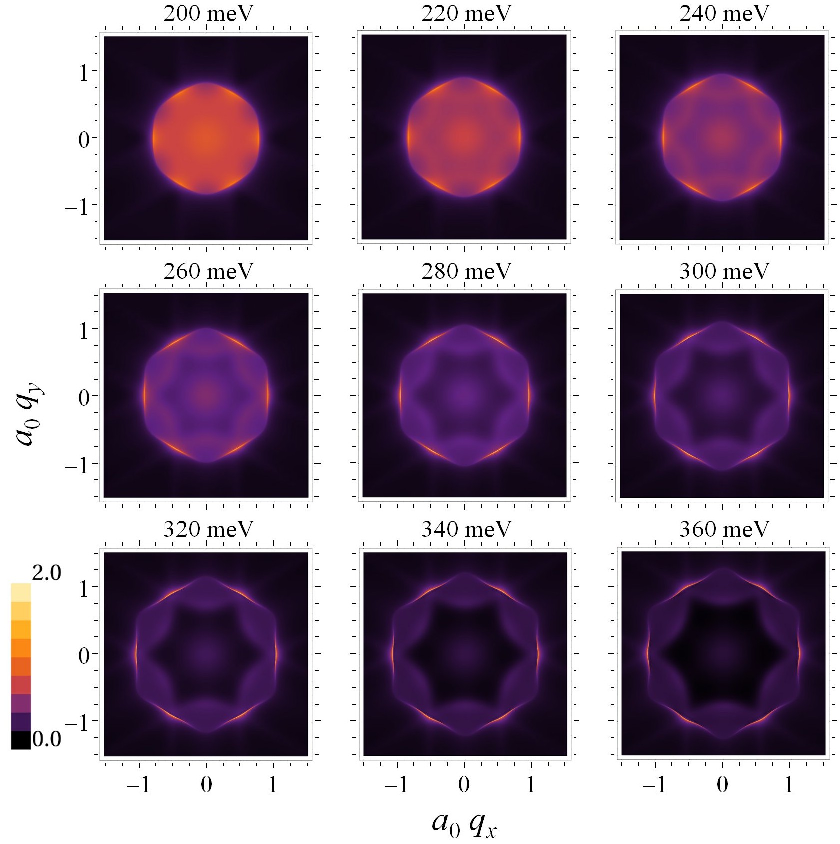
Figure 3: (Color online) QPI patterns $\Delta\rho({\bf{q}},\omega)$ at different energies $\omega$ for a dynamic magnetic impurity, with parameters $A^{2}=2.23$, $\mu=100$ meV, $U/v_{F}=0.3$, $\epsilon_{d}/v_{F}=-0.1$, and $g/v_{F}=0.168$.

Cuts through the QPI along the $\Gamma$–$K$ and $\Gamma$–$M$ directions shown in Fig. 4 allow a more detailed analysis of the high-energy behavior. One observes that the shape of the Hubbard satellites is manifest as a non-montonic intensity variation of the QPI peaks with energy, in contrast to what would be observed for non-magnetic impurities (see Appendix B). Such a feature is reminiscent of the experimental findings in Ref. Okada et al., 2011. We note that, in a more complete modelling of the impurity, non-monotonic behavior could also arise from excited crystal-field states of the magnetic impurity.

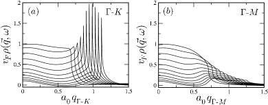
Figure 4: Cuts through the QPI signal for a dynamic magnetic impurity along (a) the $\Gamma$–$K$ direction, and (b) the $\Gamma$–$M$ direction, for a system with the same parameters as in Fig. 3. Energies shown are from 160 meV–360 meV in steps of 20 meV in order of increasing peak position.

IV.1.2 Universal Kondo regime, $\omega\sim T_{\rm K}$

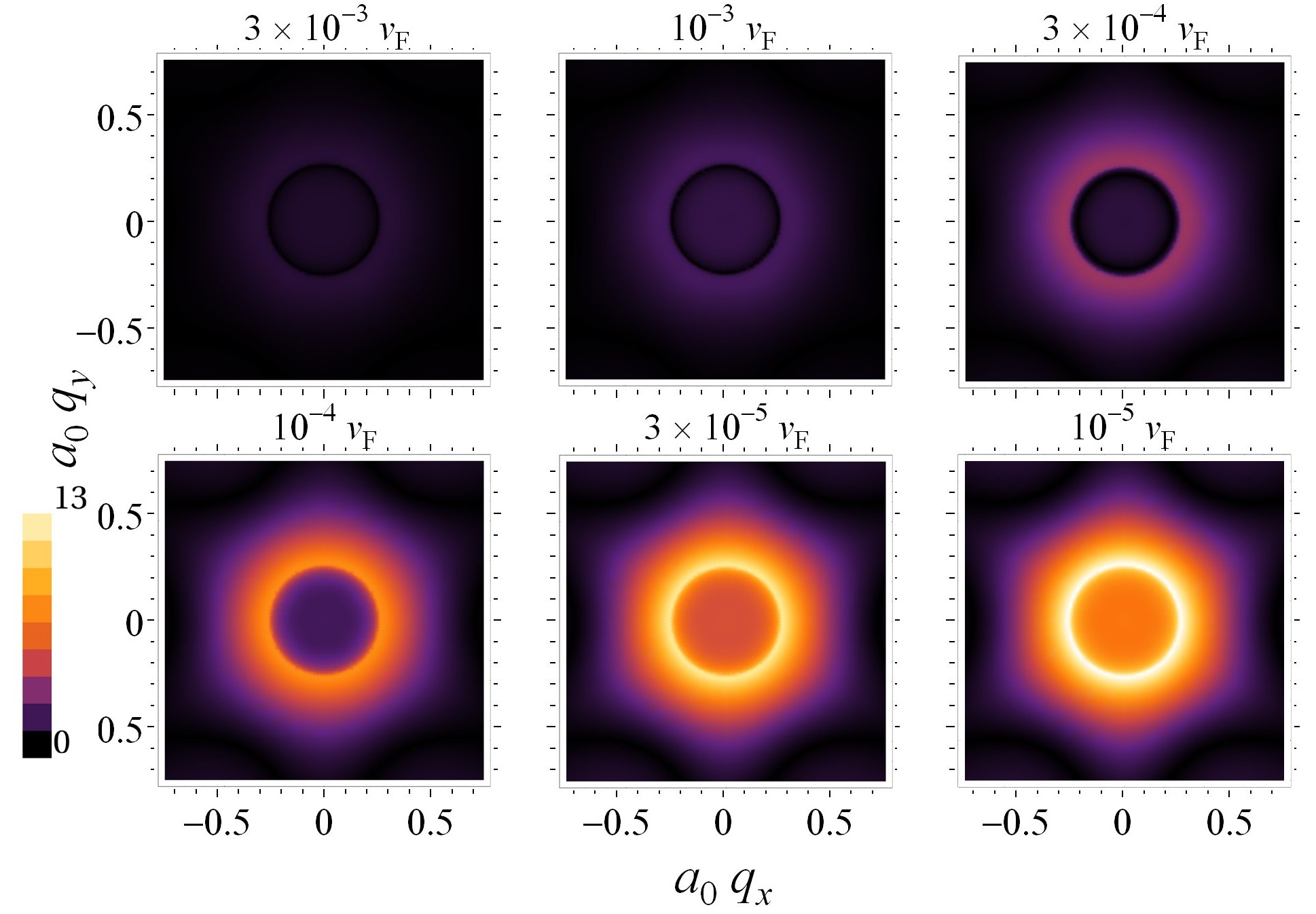
Figure 5: (color online) QPI patterns $|\Delta\rho({\bf{q}},\omega)|$ for a dynamic magnetic impurity in the low-energy Kondo regime, with the same parameters as Fig. 3, but now with scanning energies very close to the Fermi level. Note the different scale as compared with Fig. 3; also, $\Delta\rho({\bf{q}},\omega)$ has sign changes, see Fig. 6.

The pronounced build-up of impurity spectral intensity in a very narrow energy window $\mathcal{O}(T_{\rm K})$ around the Fermi level is the characteristic signature of the Kondo effect [see Fig. 2(b)]. This results in a similarly characteristic evolution of the QPI pattern at low energies.

For the parameters used in Fig. 3, the Kondo scale is $T_{\rm K}\approx 10^{-4}v_{F}$, and so we probe the system around these energies in Fig. 5. The intensity of the QPI peaks indeed grows rapidly in this regime due to the Kondo effect. This is further highlighted in Fig. 6, where cuts through the QPI pattern are shown. (We note the different scales in Figs. 3 and 5 as well as Figs. 4 and 6, respectively.)

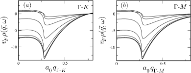
Figure 6: Cuts through the QPI signal for a dynamic magnetic impurity in the low-energy Kondo regime along (a) the $\Gamma$–$K$ direction, and (b) the $\Gamma$–$M$ direction, for a system with the same parameters as in Fig. 3. Energies shown are $\omega/v_{F}=3\times 10^{-3}$, $10^{-3}$, $3\times 10^{-4}$, $10^{-4}$, $3\times 10^{-5}$, $10^{-5}$, $3\times 10^{-6}$, $10^{-6}$ in order of increasing peak intensity.

At low energies in the Kondo regime, there is a universal scaling collapse of the impurity Green function in terms of $\omega/T_{K}$ and $T/T_{K}$. As in this regime (and in the scaling limit) the free Green function $\hat{G}^{(0)}({\bf{k}},\omega)$ is essentially independent of energy (and strictly independent of temperature) one naturally expects universality and scaling of the entire QPI pattern. As we show in Fig. 7 this is indeed the case.

The $T=0$ peak intensity for different choices of the system parameters, and thus the Kondo temperature, is shown in Fig. 7(a). At low energies the data is well described by

$$\frac{\rho({\bf{q}}_{p},\omega,T=0)}{\tilde{\rho}({\bf{q}}_{p})} = 1-a\left(\frac{\omega}{T_{\rm K}}\right)^{2},\quad\omega\ll T_{\rm K},$$

$${\rm{with}}\quad\tilde{\rho}({\bf{q}}_{p}) = \rho({\bf{q}}_{p},\omega=0,T=0)$$ (18)

where ${\bf{q}}_{p}$ denotes the scattering vector of the peak. The quadratic behavior reflects the Fermi liquid nature of the Kondo ground state. Similarly, at elevated energies the asymptote is given by

$$\frac{\rho({\bf{q}}_{p},\omega,T=0)}{\tilde{\rho}({\bf{q}}_{p})}\sim\frac{1}{\ln(a^{\prime}|\omega|/T_{K})^{2}},\quad T_{\rm K}\ll\omega\ll v_{F},$$ (19)

corresponding to spin-scattering processes in the vicinity of the local-moment fixed point. These forms reflect universality in the scaling limit ($T_{\rm K}\to 0$) of the Kondo impurity, with universal coefficients $a,a^{\prime}=\mathcal{O}(1)$. Corrections arise from two sources: There is a leading linear-in-$\omega$ term in Eq. (IV.1.2) because the QPI pattern involves both real and imaginary parts of $G^{d}_{\sigma}(\omega)$, and the real part of the self energy is generically non-zero. The linear energy variation of $\rho^{(0)}$ contributes to this linear term as well (this is where an explicit $\mu$ dependence enters), and it also causes deviations in Eq. (19). These corrections are suppressed by the factor $\omega/{\rm min}(|\mu|,v_{F})$ and are small for the data shown in Fig. 7(a).

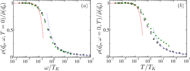
Figure 7: (color online) (a) Scaling collapse of the $T=0$ QPI peak intensity at low energies for different bare parameters and hence different Kondo temperatures, $T_{\rm K}$. The peak position at $\textbf{q}=\textbf{q}_{p}$ is essentially pinned at low energies (see Fig. 6) as $\mu/v_{F}=0.1$ is kept fixed. Circles: $(U/v_{F},\epsilon/v_{F},g/v_{F})=(0.2,-0.1,0.126)$, $T_{\rm K}\approx 10^{-2}$ K; Squares: $(0.2,-0.1,0.168)$, $T_{\rm K}\approx 2$ K; Diamonds: $(0.3,-0.15,0.126)$, $T_{\rm K}\approx 6\times 10^{-5}$ K; Crosses: $0.3,-0.15,0.168)$, $T_{\rm K}\approx 0.1$ K. For illustration we have also plotted (Green Stars) the peak intensity for $(U/v_{F},\epsilon/v_{F},g/v_{F})=(0.2,-0.1,0.175)$ and a different $\mu/v_{F}=0.137$, yielding $T_{\rm K}\approx 20$ K. Red dashed line: Low-energy asymptote Eq. (IV.1.2). Blue dotted line: High-energy asymptote Eq. (19). (b) Scaling collapse of the $\omega=0$ peak intensity at low temperatures for the same systems as in (a). Red dashed line: Low-temperature asymptote Eq. (20). Blue dotted line: High-temperature asymptote Eq. (21). Deviations from scaling at higher $T$ become apparent for the $T_{\rm K}=20$ K data.

The temperature scaling of the $\omega=0$ peak intensity is shown in Fig. 7(b). In the low-temperature limit one finds

$$\frac{\rho({\bf{q}}_{p},\omega=0,T)}{\tilde{\rho}({\bf{q}}_{p})}=1-b\left(\frac{T}{T_{\rm K}}\right)^{2},\quad T\ll T_{\rm K},$$ (20)

characteristic of Fermi-liquid behavior. Indeed, we find that the Fermi liquid relation $a/b=3/\pi^{2}$ is well-satisfied from our numerical calculations. Similarly to Eq. (19) the spin-flip scattering processes in the vicinity of the local-moment fixed point lead to the temperature dependence

$$\frac{\rho({\bf{q}}_{p},\omega=0,T)}{\tilde{\rho}({\bf{q}}_{p})}\sim\frac{1}{\ln(b^{\prime}T/T_{\rm K})^{2}},\quad T_{\rm K}\ll T\ll v_{F},$$ (21)

where $b,b^{\prime}=\mathcal{O}(1)$ are again universal. Deviations from universality arise as above; they are visible for the highest-$T_{\rm K}$ data in Fig. 7(b).

The characteristic feature of the Kondo effect is thus the rapid increase of QPI peak intensity as the scanning energy approaches the Fermi level, together with the (approximate) scaling collapse in $\omega/T_{\rm K}$ and $T/T_{\rm K}$. These features should be readily observable provided that experiments are performed at temperatures of order $T_{\rm K}$ or lower.

Finally, we comment briefly on the case where a (small) magnetic field acts on the dynamic magnetic impurity. Since $T^{0}_{\textbf{k},\textbf{k}^{\prime}}(\omega)$ and the impurity model in the absence of a field is SU(2) symmetric, it is sufficient to discuss the spin-summed impurity spectral function. For small fields $\mathcal{O}(T_{K})$, this is known to develop a split Kondo resonance,Hewson (1993) signatures of which should show up in QPI. For larger fields $\gg T_{K}$, the Kondo effect is destroyed entirely, and only the high-energy Hubbard satellites remain thus leading to a behavior qualitatively similar to Fig. 3.

IV.2 Local-moment phase

In the local-moment regime, realized if the chemical potential is tuned to the Dirac point $\mu=0$ (unless the Kondo coupling and asymmetry is very strong), there is no low-energy Kondo resonance in the impurity spectral function, although the Hubbard satellites remain [see Fig. 2(a)].

As a result, the high-energy features of the QPI pattern are essentially the same as those in Figs. 3, 4, but there is no build-up of QPI peak intensity in the vicinity of the Fermi level. The same applies to the situation with non-zero $\mu$ but temperatures $T\gg T_{\rm K}$.

V Conclusions

In this work we have studied modulations in the LDOS caused by dilute magnetic impurities on the surface of 3D TIs. Despite the coupling of orbital and spin degrees of freedom in the helical surface metal and hexagonal warping due to the underlying TI lattice structure, the quantum impurity problem itself is of conventional type, such that Kondo screening is generically present in the low-temperature limit (unless the chemical potential is tuned to the Dirac point).

We identified the energy dependence of the QPI peak intensity as the fingerprint of dynamic magnetic impurities (as opposed to non-magnetic or spin-polarized impurites, see appendix). At elevated energies, non-monotonic QPI peak intensity for scanning energies is observed due to Hubbard satellites in the impurity spectral function. At low scanning energies, Kondo screening of the impurity produces a strong build-up of QPI peak intensity, whose energy and temperature dependence are universal functions of $\omega/T_{\rm K}$ and $T/T_{\rm K}$.

However, the momentum dependence of the QPI signal (at fixed energy) is identical for the different types of impurities, due to the fact that only the spin-diagonal part of the T matrix produces modulations in the charge channel.Guo and Franz (2010) This casts doubts on the interpretation of the experimental data given in Ref. Okada et al., 2011, where the magnetic character of dilute Fe impurities was made responsible for the appearance of new QPI wavevectors. At present, the source of this QPI signal is unclear, and more systematic studies are called for.

Appendix A Local Green function and symmetries

Here we consider the form of the local free Green function, and show explicitly that its off-diagonal components vanish. The inverse Green function for Matsubara frequencies in spin-space reads

$$\hat{G}^{0}(i\omega_{n},{\bf{k}})^{-1}=\left(\begin{array}[]{cc}i\omega_{n}+\mu-A^{2}k^{3}\cos 3\phi_{\bf{k}}&-v_{F}\left(k_{y}+ik_{x}\right)\\ -v_{F}\left(k_{y}-ik_{x}\right)&i\omega_{n}+\mu+A^{2}k^{3}\cos 3\phi_{\bf{k}}\end{array}\right)$$ (22)

where the local Green function assumes the form

$$\hat{G}^{0}(i\omega_{n},r=0)=\int\frac{kdk}{2\pi}\int\frac{d\phi}{2\pi}\frac{1}{(i\omega_{n}+\mu)^{2}-v_{F}^{2}(k^{2}+A^{4}k^{6}\cos^{2}3\phi)}\left(\begin{array}[]{cc}i\omega_{n}+\mu-A^{2}k^{3}\cos 3\phi&v_{F}\left(k\sin\phi+ik\cos\phi\right)\\ v_{F}\left(k\sin\phi-ik\cos\phi\right)&i\omega_{n}+\mu+A^{2}k^{3}\cos 3\phi\end{array}\right)$$ (23)

The off-diagonal terms do not survive the angular integration, such that the remaining diagonal components simplify to

$$\hat{G}^{0}(i\omega_{n},r=0)=\mathbb{I}\int\frac{kdk}{2\pi}\int\frac{d\phi}{2\pi}\frac{i\omega_{n}+\mu}{(i\omega_{n}+\mu)^{2}-v_{F}^{2}(k^{2}+A^{4}k^{6}\cos^{2}3\phi)}$$ (24)

This immediately allows one to read off the energy eigenvalues in Eq. (5).

Appendix B QPI from non-magnetic impurities

For completeness, we show here the QPI signal of non-magnetic impurities, which has largely been calculated and discussed in Refs. Roushan et al., 2009; Guo and Franz, 2010; Lee et al., 2009b; Okada et al., 2011; Zhou et al., 2009.

B.1 Scattering potential

The TI surface metal with a non-magnetic scalar impurity or potential scatterer is described by $H=H_{0}+H_{V}$, with

$$H_{V}=V\sum_{\sigma}\Psi^{\dagger}_{\sigma}(r=0)\Psi^{\phantom{\dagger}}_{\sigma}(r=0)\;,$$ (25)

The exact T matrix is

$$\hat{T}_{\textbf{k},\textbf{k}^{\prime}}(\omega)=\frac{1}{N}\frac{V}{1-Vf_{\omega,\mu}}\mathbb{I}=\frac{1}{N}T^{0}(\omega)\,\mathbb{I}\;,$$ (26)

with $f_{\omega,\mu}$ given in Eq. (8), while lowest-order Born approximation (valid for small $V$) corresponds to $T^{0}(\omega)=V$ which is real and constant. The QPI pattern in this approximation is displayed in Fig. 1(b).

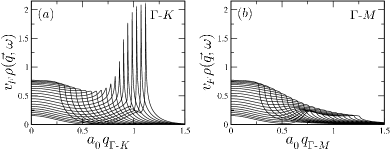
Figure 8: Cuts through the QPI signal for a scalar impurity along (a) the $\Gamma$–$K$ direction, and (b) the $\Gamma$–$M$ direction, for a system with $\mu=100$ meV and a potential scattering strength $V/v_{F}=0.1$. Energies shown are from 0 meV–360 meV in steps of 20meV in order of increasing peak position (20 meV $\simeq 0.027v_{F}$).

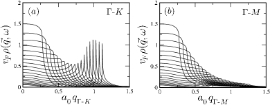
Figure 9: Cuts through the QPI signal for a resonant level along (a) the $\Gamma$–$K$ direction, and (b) the $\Gamma$–$M$ direction, for a system with $\mu=100$ meV, $U=0$, $\epsilon_{d}/v_{F}=-0.1$ and $g/v_{F}=0.168$. Energies shown are from 0 meV–360 meV in steps of 20 meV in order of increasing peak position.

Since impurities are often not weak, the Born approximation may be insufficient. Results using the full T matrix, which now includes a small imaginary part, are plotted in Fig. 8 for $V/v_{F}=0.1$. We observe that the intensity of the peak along the $\Gamma$–$K$ direction simply increases monotonically as the scanning energy $|\omega|$ increases (for both $\omega>0$ and $\omega<0$).

B.2 Resonant level

A so-called resonant level impurity is obtained by setting $U=0$ in Eq. (14), physically corresponding to a mixed-valent impurity atom. Then, the impurity spectral function consists of a single peak centered around $\omega=\epsilon_{d}$. In contrast to the scalar impurity discussed above the T matrix of the resonant level possesses an appreciable imaginary part (see Eq. (17) with $\Sigma^{d}=0$).

Cuts through the QPI pattern along the $\Gamma$–$K$ and $\Gamma$–$M$ directions at different scanning energies are plotted in Fig. 9 for $\mu=100$ meV, $\epsilon_{d}/v_{F}=-0.1$ and $g/v_{F}=0.168$. For this resonant level, the intensity of the peak is reminiscent of the high-energy response produced by a Kondo impurity obtained for $U>0$ (simple charge fluctuations are responsible for the evolution of the QPI signal at high energies in both cases). However, crucially there is no build-up of QPI intensity at low energies, since there is no Kondo effect (see by contrast Fig. 6).

Appendix C QPI from static magnetic impurities

The simplest model for a static, i.e. polarized, magnetic impurity is a local magnetic field, corresponds to a spin-dependent version of the potential scattering case considered above. Thus we have $H=H_{0}+H_{h}$, with

$$H_{h}=h\sum_{\sigma}\Psi^{\dagger}_{\sigma}(r=0)\sigma_{z}\Psi^{\phantom{\dagger}}_{\sigma}(r=0)\;.$$ (27)

Within the Born approximation, the T matrix is then

$$\hat{T}_{{\bf{k}},{\bf{k}}^{\prime}}\approx\frac{h}{N}\sigma_{z}\;,$$ (28)

i.e. $T^{1}(\omega)=h$, such that there is no response in QPI due to Eq. (13). Beyond the lowest-order Born approximation, a (weak) response similar to that of a potential scatterer is induced, see Refs. Liu et al., 2009; Guo and Franz, 2010; Zhou et al., 2009.

References

- Kane and Mele (2005) C. L. Kane and E. J. Mele, Phys. Rev. Lett. 95, 226801 (2005).
- Bernevig et al. (2006) B. A. Bernevig, T. L. Hughes, and S.-C.Zhang, Science 314, 1757 (2006).
- König et al. (2007) M. König, S. Wiedmann, C. Brüne, A. Roth, H. Buhmann, L. W. Molenkamp, X.-L. Qi, and S.-C. Zhang, Science 318, 766 (2007).
- Fu et al. (2007) L. Fu, C. L. Kane, and E. J. Mele, Phys. Rev. Lett. 98, 106803 (2007).
- Moore and Balents (2007) J. E. Moore and L. Balents, Phys. Rev. B 75, 121306 (2007).
- Qi et al. (2008) X.-L. Qi, T. L. Hughes, and S.-C. Zhang, Phys. Rev. B 78, 195424 (2008).
- Roy (2009) R. Roy, Phys. Rev. B 79, 195322 (2009).
- Bardarson et al. (2007) J. H. Bardarson, J. Tworzydlo, P. W. Brouwer, and C. W. J. Beenakker, Phys. Rev. Lett. 99, 106801 (2007).
- Nomura et al. (2007) K. Nomura, M. Koshino, and S. Ryu, Phys. Rev. Lett. 99, 146806 (2007).
- Roushan et al. (2009) P. Roushan, J. Seo, C. V. Parker, Y. S. Hor, D. Hsieh, D. Qian, A. Richardella, M. Z. Hasan, R. J. Cava, and A. Yazdani, Nature 460, 1106 (2009).
- Alpichshev et al. (2010) Z. Alpichshev, J. G. Analytis, J.-H. Chu, I. R. Fisher, Y. L. Chena, Z. X. Shen, A. Fang, and A. Kapitulnik, Phys. Rev. Lett. 104, 016401 (2010).
- Zhang et al. (2009) T. Zhang, P. Cheng, X. Chen, J.-F. Jia, X. Ma, K. He, L. Wang, H. Zhang, X. Dai, Z. Fang, et al., Phys. Rev. Lett. 103, 266803 (2009).
- Okada et al. (2011) Y. Okada, C. Dhital, W. Zhou, E. D. Huemiller, H. Lin, S. Basak, A. Bansil, Y.-B. Huang, H. Ding, Z. Wang, et al., Phys. Rev. Lett. 106, 206805 (2011).
- Hsieh et al. (2008) D. Hsieh, D. Qian, L. Wray, Y. Xia, Y. S. Hor, R. J. Cava, and M. Z. Hasan, Nature 452, 970 (2008).
- Xia et al. (2009) Y. Xia, D. Qian, D. Hsieh, L. Wray, A. Pal, H. Lin, A. Bansil, D. Grauer, Y. S. Hor, R. J. Cava, et al., Nature Phys. 5, 398 (2009).
- Crommie et al. (1993) M. F. Crommie, C. P. Lutz, and D. M. Eigler, Nature 363, 524 (1993).
- Lee et al. (2009a) J. Lee, K. Fujita, A. R. Schmidt, C. K. Kim, H. Eisaki, S. Uchida, and J. C. Davis, Science 325, 1099 (2009a).
- Liu et al. (2009) Q. Liu, C.-X. Liu, C. Xu, X.-L. Qi, and S.-C. Zhang, Phys. Rev. Lett. 102, 156603 (2009).
- Zhou et al. (2009) X. Zhou, C. Fang, W.-F. Tsai, and J.-P. Hu, Phys. Rev. B 80, 245317 (2009).
- Guo and Franz (2010) H.-M. Guo and M. Franz, Phys. Rev. B 81, 041102 (2010).
- Hewson (1993) A. C. Hewson, The Kondo Problem to Heavy Fermions (Cambridge University Press, 1993).
- Zitko (2010) R. Zitko, Phys. Rev. B 81, 241414(R) (2010).
- Tran and Kim (2010) M.-T. Tran and K.-S. Kim, Phys. Rev. B 82, 155142 (2010).
- Lee et al. (2009b) W.-C. Lee, C. Wu, D. P. Arovas, and S.-C. Zhang, Phys. Rev. B 80, 245439 (2009b).
- (25) P. Thalmeier and A. Akbari, preprint arXiv:1210.2222.
- Fu (2009) L. Fu, Phys. Rev. Lett. 103, 266801 (2009).
- Hsieh et al. (2009) D. Hsieh, Y. Xia, D. Qian, L. Wray, J. H. Dil, F. Meier, J. Osterwalder, L. Patthey, J. G. Checkelsky, N. P. Ong, et al., Nature 406, 1101 (2009).
- Chen et al. (2009) Y. L. Chen, J. G. Analytis, J.-H. Chu, Z. K. Liu, S.-K. Mo, X. L. Qi, H. J. Zhang, D. H. Lu, X. Dai, Z. Fang, et al., Science 325, 178 (2009).
- (29) Recall that our model is defined in the continuum; the short-distance (or ultraviolet) cutoff is effectively set by .
- Capriotti et al. (2003) L. Capriotti, D. J. Scalapino, and R. D. Sedgewick, Phys. Rev. B 68, 014508 (2003).
- Fritz and Vojta (2005) L. Fritz and M. Vojta, Phys. Rev. B 72, 212510 (2005).
- Bulla et al. (2008) R. Bulla, T. Costi, and T. Pruschke, Rev. Mod. Phys. 80, 395 (2008).
- Oliveira and Oliveira (1994) W. C. Oliveira and L. N. Oliveira, Phys. Rev. B 49, 11986 (1994).
- Peters et al. (2006) R. Peters, T. Pruschke, and F. B. Anders, Phys. Rev. B 74, 245114 (2006).
- Weichselbaum and von Delft (2007) A. Weichselbaum and J. von Delft, Phys. Rev. Lett. 99, 076402 (2007).
- Withoff and Fradkin (1990) D. Withoff and E. Fradkin, Phys. Rev. Lett. 64, 1835 (1990).
- Gonzalez-Buxton and Ingersent (1998) C. Gonzalez-Buxton and K. Ingersent, Phys. Rev. B 57, 14254 (1998).
- Bulla et al. (2000) R. Bulla, M. T. Glossop, D. E. Logan, and T. Pruschke, J. Phys.: Condens. Matter 12, 4899 (2000).
- Vojta and Fritz (2004) M. Vojta and L. Fritz, Phys. Rev. B 70, 094502 (2004).
- Fritz and Vojta (2004) L. Fritz and M. Vojta, Phys. Rev. B 70, 214427 (2004).
- Vojta and Bulla (2002) M. Vojta and R. Bulla, Phys. Rev. B 65, 014511 (2002).
- Vojta et al. (2010) M. Vojta, L. Fritz, and R. Bulla, EPL 90, 27006 (2010).
- van Heumen and Golden (2012) E. van Heumen and M. Golden, Private communication (2012).