Conservation Laws
in the Modeling of Moving Crowds

Abstract

Models for crowd dynamics are presented and compared. Well posedness results allow to exhibit the existence of optimal controls in various situations. A new approach not based on partial differential equations is also briefly considered.

Rinaldo M. Colombo

Department of Mathematics, Brescia University, Brescia, Italy

Mauro Garavello

Department of Mathematics and Applications, Milano – Bicocca University, Milano, Italy

Magali Lécureux-Mercier

Technion, Israel Institute of Technology, Haifa, Israel

Nikolay Pogodaev

Russian Academy of Sciences, Irkutsk, Russia

1 Introduction

From a macroscopic viewpoint, a moving crowd can be described through its density $\rho=\rho(t,x)$, a function of time $t\in{\mathbb{R}}^{+}$ and space $x\in{\mathbb{R}}^{2}$ attaing values in $[0,1]$. In standard situations, the number of pedestrians is conserved, so that $\int_{{\mathbb{R}}^{2}}\rho(t,x)\mathinner{\mathrm{d}{x}}$ is independent of $t$. Hence, it is natural to use the conservation law

$$\partial_{t}\rho+\mathinner{\rm div}_{x}(\rho\,V)=0\,.$$ (1)

Any model of this kind depends on the speed law that defines the velocity $V$ of the crowd as a function of $t$, $x$, $\rho$, $\ldots$ A simple version of (1) is obtained assigning

$$V=v(\rho)\,\vec{v}(x)\quad\mbox{ with }\quad\begin{array}[]{l}v\in\mathbf{C}^{2}([0,1];{\mathbb{R}}^{+})\mbox{ non increasing and }v(1)=0\,,\\ \vec{v}\in\mathbf{C}^{2}({\mathbb{R}}^{2};\mathbb{S}^{1})\,.\end{array}$$ (2)

In this case, Kružkov Theorem [24, Theorem 1] applies and ensures that the Cauchy problem for (1)–(2) has a unique solution in $\mathbf{C}^{0,1}\left({\mathbb{R}}^{+};{\mathbf{L}^{1}}({\mathbb{R}}^{2};[0,1])\right)$ which depends Lipschitz continuously from the data and, by [12, Theorem 2.6], also from $v$ and $\vec{v}$.

According to (2), at time $t$ the pedestrian at $x$ moves along a prescribed trajectory, an integral curve of $\vec{v}$, with a speed $v(\rho)$ that depends on $\rho$ evaluated at point $x$ and time $t$. On the contrary, Section 2 is devoted to (1) with the speed of the individual at $x$ depending on an average of the density $\rho$ in a neighborhood of $x$. The resulting model has a rich analytical structure, the solutions being also differentiable with respect to the data and to the speed law.

In Section 3 the direction chosen by the pedestrian at $x$ depends from an average of the density gradient $\nabla\rho$ around $x$, while his/her speed depends from $\rho$ evaluated at $x$. The resulting solutions display qualitative properties usually seen in context where individuals have a proper volume such as the Braess paradox [3] and the formation of queues [23].

If the various individuals have different destinations then it is possible to subdivide the crowd under consideration into different, say $n$, populations with densities $\rho_{1},\ldots,\rho_{n}$, each having a different destination. The resulting model

$$\partial_{t}\rho_{i}+\mathinner{\rm div}_{x}(\rho_{i}\,V_{i})=0\qquad i=1,\ldots,n$$ (3)

consists of a system of conservation laws that, when $n=1$, reduces to (1). The results in both Section 2 and Section 3 can be extended to this more general setting.

Finally, Section 4 approaches the problem of driving a crowd with a few moving individuals. First, a model based on (1) is recalled and then an approach based on differential inclusions is presented. The latter approach, developed following [5, 6], neglects the crowd internal dynamics and allows for a simpler analytical framework.

We refer for instance to [2] for an account of the fast development of the recent macroscopic modeling of crowd dynamics. Moreover, measure valued conservation laws were considered in [18, 26]; the results in [25] deal with constrained velocity models; various 1D attempts are found in [1, 15, 16, 20, 21]. Throughout, for the basic results in the theory of conservation laws we refer to [4, 19].

2 NonLocal Speed Choice

Consider (1) with the nonlocal speed law

$$V(\rho)=v\left(\rho(t)*\eta\right)\,\vec{v}\,.$$ (4)

Here, the speed $v$ at time $t$ of the pedestrian at $x$ depends on the averaged density $\left(\rho(t)*\eta\right)(x)=\int_{{\mathbb{R}}^{2}}\rho(t,x-y)\,\eta(y)\,\mathinner{\mathrm{d}{y}}$. The direction of the velocity is given by the (fixed) vector $\vec{v}(x)$.

For simplicity, we state the results below in ${\mathbb{R}}^{2}$. However, the case where the region available to the crowd is constrained by, say, walls or doors can be easily recovered in the present framework, along the technique used in [7, 8]

As is typical whenever Kružkov techniques apply, space dimension $2$ plays no role and the results below can be extend to ${\mathbb{R}}^{n}$.

Existence and uniqueness of a solution to the Cauchy problem for (1)–(4) follow from the next result.

Theorem 2.1.

[9, Proposition 4.1], [10, Theorem 2.2] Let $v\in(\mathbf{C}^{2}\cap{\mathbf{W}^{2,\infty}})({\mathbb{R}};{\mathbb{R}})$, $\vec{\nu}\in(\mathbf{C}^{2}\cap{\mathbf{W}^{2,1}})({\mathbb{R}}^{2};{\mathbb{R}}^{2})$, $\eta\in(\mathbf{C}^{2}\cap{\mathbf{W}^{2,\infty}})({\mathbb{R}}^{2};{\mathbb{R}})$. Assume $\rho_{o}\in({\mathbf{L}^{1}}\cap{\mathbf{L}^{\infty}}\cap\mathbf{BV})({\mathbb{R}}^{2};{\mathbb{R}^{+}})$. Then, (1)–(4) with initial condition $\rho_{o}$ admits a unique weak entropy solution $\rho\in\mathbf{C}^{0}\left({\mathbb{R}^{+}};{\mathbf{L}^{1}}({\mathbb{R}}^{2};{\mathbb{R}^{+}})\right)$. Furthermore, we have the estimate $\displaystyle{\left\|\rho(t)\right\|}_{{\mathbf{L}^{\infty}}}\leq{\left\|\rho_{o}\right\|}_{{\mathbf{L}^{\infty}}}e^{Ct}$, where the constant $C$ depends on $v$, $\vec{\nu}$ and $\eta$.

The definition of weak entropy solutions is based on Kružkov notion [24, Definition 1], see also [9, 10]. The proof relies on a contraction argument based on the key estimates provided by [12, Theorem 2.6].

Another contraction argument, based on tools from optimal transport theory, allows to extend the above result to the measure valued setting in [17]. (Below, $\mathcal{M}^{+}({\mathbb{R}}^{+})$ is the set of positive Radon measures on ${\mathbb{R}}^{2}$).

Theorem 2.2.

[17, Theorem 1.1] Assume $v\in({\mathbf{L}^{\infty}}\cap\mathinner{\mathbf{missing}}{Lip})({\mathbb{R}};{\mathbb{R}})$, $\vec{\nu}\in({\mathbf{L}^{\infty}}\cap\mathinner{\mathbf{missing}}{Lip})({\mathbb{R}}^{2};{\mathbb{R}}^{2})$, $\eta\in({\mathbf{L}^{\infty}}\cap\mathinner{\mathbf{missing}}{Lip})({\mathbb{R}}^{2};{\mathbb{R}^{+}})$. Let $\rho_{o}\in\mathcal{M}^{+}({\mathbb{R}}^{2})$. Then, there exists a unique weak measure valued solution $\rho\in{\mathbf{L}^{\infty}}({\mathbb{R}^{+}};\mathcal{M}^{+}({\mathbb{R}}^{2}))$ to (1)–(4) with initial condition $\rho_{o}$. If furthermore $\rho_{o}\in{\mathbf{L}^{1}}({\mathbb{R}}^{2};{\mathbb{R}^{+}})$, then $\rho\in\mathbf{C}^{0}\left({\mathbb{R}}^{+};{\mathbf{L}^{1}}({\mathbb{R}}^{2};{\mathbb{R}^{+}})\right)$.

In general, in (1)–(4) no a priori uniform ${\mathbf{L}^{\infty}}$ bound on the density is possible. Indeed, assume that the density is $1$ all along the trajectory of the pedestrian at $x$. The averaged density around $x$ may well be less than $1$, forcing the pedestrian to proceed and, hence, leading to a increase in the density. This behavior can be related to the rise of panic, see [15, 16]. In the literature, values of $\rho$ of up to 10 individuals per square meter were measured, see for instance [22].

Aiming at preventing the insurgence of these phenomena, it is natural to consider control problems where functionals of the density of the type

$$J_{T}(\rho_{o})=\int_{0}^{T}\int_{\Omega}f\left(\rho(t,x)\right)\,\mathinner{\mathrm{d}{x}}\,\mathinner{\mathrm{d}{t}}\quad\mbox{where }\rho\mbox{ solves \eqref{eq:1}--\eqref{eq:4}}\mbox{ with datum }\rho_{o}$$ (5)

have to be minimized. Here, $\Omega$ is the region where the density needs to be controlled and $f$ is a $\mathbf{C}^{1}$ function weighing $0$ on acceptable densities and quickly increasing when $\rho$ approaches dangerous values. Necessary conditions for the minima of (5) are available once the differentiability of the solution to (1)–(4) with respect to the initial datum is proved. This motivates the following result.

Theorem 2.3.

[9, Theorem 4.2] [10, Theorem 2.2] Let $\rho_{o}\in({\mathbf{W}^{2,\infty}}\cap{\mathbf{W}^{2,1}})({\mathbb{R}}^{2};{\mathbb{R}^{+}})$, $r_{o}\in({\mathbf{W}^{1,1}}\cap{\mathbf{L}^{\infty}})({\mathbb{R}}^{2};{\mathbb{R}})$. Assume $v\in(\mathbf{C}^{4}\cap{\mathbf{W}^{2,\infty}})({\mathbb{R}};{\mathbb{R}})$, $\vec{\nu}\in(\mathbf{C}^{3}\cap{\mathbf{W}^{2,1}})({\mathbb{R}}^{2};{\mathbb{R}}^{2})$, $\eta\in(\mathbf{C}^{3}\cap{\mathbf{W}^{2,\infty}})({\mathbb{R}}^{2};{\mathbb{R}^{+}})$. Then, there exists a unique weak entropy solution $r\in\mathbf{C}^{0}({\mathbb{R}}^{+};{\mathbf{L}^{1}}\left({\mathbb{R}}^{2};{\mathbb{R}})\right)$ to the Cauchy problem

$$\partial_{t}r+\mathinner{\rm div}(r\,v(\rho*\eta)\,\vec{\nu}(x))=-\mathinner{\rm div}(\rho\,v^{\prime}(\rho*\eta)\,\vec{\nu}(x))\,,\qquad r(0)=r_{o}\,.$$ (6)

Furthermore, for all $\rho_{o}\in({\mathbf{W}^{2,1}}\cap{\mathbf{W}^{2,\infty}})({\mathbb{R}}^{2};{\mathbb{R}^{+}})$ and $r_{o}\in({\mathbf{W}^{1,1}}\cap{\mathbf{L}^{\infty}})({\mathbb{R}}^{2};{\mathbb{R}})$, call $\rho_{h}$ the solution to (1)–(4) with initial datum $\rho_{o}+hr_{o}$. Then, for all $t\in{\mathbb{R}}^{+}$,

$$\lim_{h\to 0}{\left\|\frac{\rho_{h}(t)-\rho(t)}{h}-r(t)\right\|}_{{\mathbf{L}^{1}}}=0$$ (7)

i.e., the solution $\rho$ to (1)–(4) is Gâteaux differentiable in $\rho_{o}$ along any direction $r_{o}$.

To prove this theorem, first the well posedness of (6) is obtained and then the limit (7) is computed. In both steps, the estimates in [12] play a key role. At present, no analog to Theorem 2.3 is available in the setting of Theorem 2.2. Indeed, a good definition of Gâteaux differentiability on the set of probability measures equipped with the Wasserstein distance of order 1 is, to our knowledge, not available.

3 NonLocal Route Choice

Consider (1) with the nonlocal speed law

$$V(\rho)=v(\rho)\,\left(\vec{\nu}(x)+\mathcal{I}(\rho)\right)\,.$$ (8)

Here, the individual in $x$ at time $t$ moves at the speed $v\left(\rho(t,x)\right)$ that depends on the density $\rho(t,x)$ evaluated at the same time $t$ and $x$. The vector $\vec{\nu}(x)\in{\mathbb{R}}^{2}$ is the preferred direction of the pedestrian at $x$, while $\mathcal{I}(\rho)(x)$ describes how the pedestrian at $x$ deviates from the preferred direction, given that the crowd distribution is $\rho$. Thus, the individual at time $t$ in $x$ is assumed to move in the direction of the vector $\vec{\nu}(x)+\left(\mathcal{I}\left(\rho(t)\right)\right)(x)$. The basic well posedness result for (1)–(8) is the following.

Theorem 3.1.

[8, Theorem 2.1, Theorem 2.2] Let the following conditions hold:

(v)

$v\in\mathbf{C}^{2}({\mathbb{R}};{\mathbb{R}})$ is non increasing, $v(0)=V$ and $v(R)=0$ for fixed $V,R>0$.

($\boldsymbol{\vec{\nu}}$)

$\vec{\nu}\in(\mathbf{C}^{2}\cap{\mathbf{W}^{1,\infty}})({\mathbb{R}}^{2};{\mathbb{R}}^{2})$ is such that $\mathinner{\rm div}\vec{\nu}\in({\mathbf{W}^{1,1}}\cap{\mathbf{W}^{1,\infty}})({\mathbb{R}}^{2};{\mathbb{R}})$.

(I)

$\mathcal{I}\in\mathbf{C}^{0}\left({\mathbf{L}^{1}}({\mathbb{R}}^{2};[0,R]);\mathbf{C}^{2}({\mathbb{R}}^{2};{\mathbb{R}}^{2})\right)$ satisfies the estimates:

1. There exists an increasing $C_{I}\in{\mathbf{L}_{loc}^{\infty}}({\mathbb{R}^{+}};{\mathbb{R}^{+}})$ such that, for all $r\in{\mathbf{L}^{1}}({\mathbb{R}}^{2};[0,R])$, ${\left\|\mathcal{I}(r)\right\|}_{{\mathbf{W}^{1,\infty}}}\!\leq C_{I}({\left\|r\right\|}_{{\mathbf{L}^{1}}})$ and ${\left\|\mathcal{\mathinner{\rm div}I}(r)\right\|}_{{\mathbf{L}^{1}}}\leq C_{I}({\left\|r\right\|}_{{\mathbf{L}^{1}}})$.

2. There exists an increasing $C_{I}\in{\mathbf{L}_{loc}^{\infty}}({\mathbb{R}^{+}};{\mathbb{R}^{+}})$ such that, for all $r\in{\mathbf{L}^{1}}({\mathbb{R}}^{2};[0,R])$, ${\left\|\nabla\mathinner{\rm div}\mathcal{I}(r)\right\|}_{{\mathbf{L}^{1}}}\leq C_{I}({\left\|r\right\|}_{{\mathbf{L}^{1}}})$.

3. There exists a constant $K_{I}$ such that for all $r_{1},r_{2}\in{\mathbf{L}^{1}}({\mathbb{R}}^{2};[0,R])$,

   $${\left\|\mathcal{I}(r_{1})-\mathcal{I}(r_{2})\right\|}_{{\mathbf{L}^{\infty}}} \leq K_{I}\cdot{\left\|r_{1}-r_{2}\right\|}_{{\mathbf{L}^{1}}}\,,$$

   $${\left\|\mathcal{I}(r_{1})-\mathcal{I}(r_{2})\right\|}_{{\mathbf{L}^{1}}}+{\left\|\mathinner{\rm div}(\mathcal{I}(r_{1})-\mathcal{I}(r_{2}))\right\|}_{{\mathbf{L}^{1}}} \leq K_{I}\cdot{\left\|r_{1}-r_{2}\right\|}_{{\mathbf{L}^{1}}}\,.$$

Choose any $\rho_{o}\in({\mathbf{L}^{1}}\cap\mathbf{BV})({\mathbb{R}}^{2};[0,R])$. Then, there exists a unique weak entropy solution $\rho\in\mathbf{C}^{0}\left({\mathbb{R}^{+}};{\mathbf{L}^{1}}({\mathbb{R}}^{2};[0,R])\right)$ to (1)–(8). Moreover, $\rho$ satisfies the bounds

$${\left\|\rho(t)\right\|}_{{\mathbf{L}^{1}}} = {\left\|\rho_{o}\right\|}_{{\mathbf{L}^{1}}}\,,\mbox{ for a.e. }t\in{\mathbb{R}^{+}}\,,$$

$$\mathinner{\rm TV}(\rho(t)) \leq \mathinner{\rm TV}(\rho_{o})\,e^{kt}+\frac{\pi}{4}te^{kt}N{\left\|q\right\|}_{{\mathbf{L}^{\infty}}([0,R])}\left({\left\|\nabla\mathinner{\rm div}\vec{\nu}\right\|}_{{\mathbf{L}^{1}}}+C_{I}({\left\|\rho_{o}\right\|}_{{\mathbf{L}^{1}}})\right)\,,$$

where $k=(2N+1){\left\|q^{\prime}\right\|}_{{\mathbf{L}^{\infty}}([0,R])}\left({\left\|\nabla\vec{\nu}\right\|}_{{\mathbf{L}^{\infty}}}+C_{I}({\left\|\rho_{o}\right\|}_{{\mathbf{L}^{1}}})\right)$. If also the speed law

$$V^{\prime}(\rho)=v^{\prime}(\rho)\,\left(\vec{\nu^{\prime}}(x)+\mathcal{I}^{\prime}(\rho)\right)$$ (9)

satisfies the same assumptions, then the solution $\rho$ to (1)–(8) and $\rho^{\prime}$ to (1)–(9), with data $\rho_{o},\rho_{o}^{\prime}\in({\mathbf{L}^{1}}\cap\mathbf{BV})({\mathbb{R}}^{2};[0,R])$, satisfy

$${\left\|\rho_{1}(t)-\rho_{2}(t)\right\|}_{{\mathbf{L}^{1}}}\! \leq \!\left(1+C(t)\right)\!{\left\|\rho_{0,1}-\rho_{0,2}\right\|}_{{\mathbf{L}^{1}}}\!+C(t)\!\left({\left\|q_{1}-q_{2}\right\|}_{{\mathbf{W}^{1,\infty}}}\!+d\left(\mathcal{I}_{1},\mathcal{I}_{2}\right)\right)$$

$$+C(t)\left({\left\|\vec{\nu}_{1}-\vec{\nu}_{2}\right\|}_{{\mathbf{L}^{\infty}}}+{\left\|\mathinner{\rm div}(\vec{\nu}_{1}-\vec{\nu}_{2})\right\|}_{{\mathbf{L}^{1}}}\right)$$

where

$$d(\mathcal{I}_{1},\mathcal{I}_{2})\!=\sup\left\{{\left\|\mathcal{I}_{1}(\rho)-\mathcal{I}_{2}(\rho)\right\|}_{{\mathbf{L}^{\infty}}}\!+{\left\|\mathinner{\rm div}\left(\mathcal{I}_{1}(\rho)-\mathcal{I}_{2}(\rho)\right)\right\|}_{{\mathbf{L}^{1}}}\!\colon\!\rho\in{\mathbf{L}^{1}}({\mathbb{R}}^{2};[0,R])\right\}.$$

The map $C\in\mathbf{C}^{0}({\mathbb{R}}^{+};{\mathbb{R}}^{+})$ vanishes at $t=0$ and depends on $\mathinner{\rm TV}(\rho_{0,1})$, ${\left\|\rho_{0,1}\right\|}_{{\mathbf{L}^{1}}}$, ${\left\|\vec{\nu}_{1}\right\|}_{{\mathbf{L}^{\infty}}}$, ${\left\|\mathinner{\rm div}\vec{\nu}_{1}\right\|}_{{\mathbf{W}^{1,1}}}$, ${\left\|q_{1}\right\|}_{{\mathbf{W}^{1,\infty}}}$, ${\left\|q_{2}\right\|}_{{\mathbf{W}^{1,\infty}}}$.

In operation research, Braess paradox states that adding extra capacity to a network can, in some cases, reduce the overall performance of the network, see [3]. A relevant problem in the design of escape routes is the planning of suitable devices that reduce the exit time. The model (1)–(8) allows to show that the careful introduction of suitable obstacles in suitable locations does indeed reduce the exit time. In fact, these obstacles reduce congested areas at the sides of the door jambs.

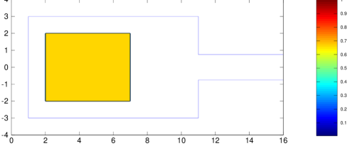
$$\begin{array}[]{@{}rcl@{}}v(\rho)&=&6(1-\rho)\,,\\ \eta(x)&=&\left[1-\left(\frac{x_{1}}{r}\right)^{2}\right]^{3}\left[1-\left(\frac{x_{2}}{r}\right)^{2}\right]^{3}\\ &&\quad\times{\chi_{[-r,r]^{2}}}(x),\\ \rho_{o}(x)&=&0.75\,{\chi_{[2,7]\times[-2,2]}}(x)\,,\\ r&=&0.6\,,\qquad\varepsilon\;\;=\;\;0.4\,.\end{array}$$ (10)

Figure 1: Initial datum and room geometry, without obstacles.

We consider a room with an exit, as in Figure 1. The vector $\vec{\nu}=\vec{\nu}(x)$ is the unit vector tangent at $x$ to the geodesic connecting $x$ to the exit and $\mathcal{I}(\rho)=-\varepsilon\,\left.\left(\nabla(\rho*\eta)\right)\middle/\sqrt{1+{\left\|\nabla(\rho*\eta)\right\|}^{2}}\right.$, see (10).

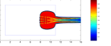
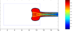
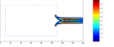
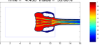
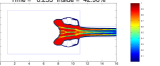
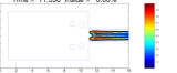
Figure 2: Solution to (1)–(8)–(10) with $\varepsilon=0.2$, at times $t=4.438$, $6.253$, $11.396$. On the first line, no obstacle is present. On the second line, $4$ columns direct the crowd flow. The exit time in the latter case is shorter than in the former one, see [7].

The careful positioning of obstacles as in the second line of Figure 2 diminishes the size of the congested region and, with the chosen initial datum, gives an exit time lower than that with the room free from any obstacle, see Figure 2.

4 Individuals Driving a Population

We finally introduce a model describing the situation in which a discrete set of isolated individuals interacts with a continuum crowd. Examples can be a (group of) predator(s) running after their preys, shepherd dogs driving a herd of sheep, or a leader attracting a group of followers to a given region. Let $\rho\in{\mathbb{R}^{+}}$ be the population density and $p\equiv(p_{1},\ldots,p_{k})\in{\mathbb{R}}^{2k}$ be the positions of the $k$ individuals. Following [11], the interaction is described by

$$\left\{\begin{array}[]{l}\partial_{t}\rho+\mathinner{\rm div}\left(\rho\,V\!\left(t,x,\rho(t,x),p(t)\right)\right)=0\,,\\ \dot{p}=\varphi\left(t,p(t),\rho(t)\right)\,.\end{array}\right.$$ (11)

Here, $\varphi$ is typically nonlocal, meaning that the individuals $p$ react to averages of quantities depending on $\rho$. The well posedness of (11) is proved in [11, Theorem 2.2], by means of Kružkov theory, the estimates in [12] and tools from the stability of ordinary differential equations.

As a first illustrating example, assume that the vector $p\in{\mathbb{R}}^{2}$ is the position of a leader (e.g. a magic piper) and $\rho$ is the density of the followers (e.g. rats). We are thus lead to consider (11) with

$$\begin{array}[]{rcl}V(t,x,\rho,p)&=&v(\rho)\,(p-x)\,e^{-{\left\|p-x\right\|}}\\ \varphi(t,\pi,\rho)&=&\left(1+(\rho*\eta)\left(p(t)\right)\right)\,\vec{{\psi}}(t)\,.\end{array}$$ (12)

The function $v$ essentially describes the speed of the followers and is, as usual, a smooth decreasing function vanishing at, say, $\rho=1$. The follower located at $x$ moves along $p(t)-x$ toward the leader, with a speed exponentially decreasing with the distance ${\left\|p-x\right\|}$ between leader and follower. The speed of the leader increases with the averaged density $\rho*\eta$, computed at the leader’s position. Indeed, we expect the leader to wait for the followers to join him when the followers’ density around him is small. The direction $\vec{\psi}$ of the leader is chosen a priori.

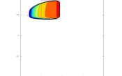
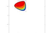
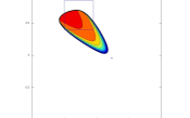
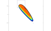
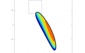
Figure 3: Solution of (11)–(12), from [11].

See Figure 3 for a numerical integration of (11)–(12) and [11] for further details.

As a further example, consider $n$ shepherd dogs, located in $p_{i}(t)\in{\mathbb{R}}^{2}$ for $i\in\{1,\ldots,n\}$ and a group of sheep of density $\rho$. The dogs have to confine the sheep within a given area. We are thus lead to consider (11) with

$$\begin{array}[]{rcl}V(t,x,\rho,p)&=&v(\rho)\,\vec{\nu}(x)+\sum_{i=1}^{n}(x-p_{i})e^{-{\left\|p_{i}-x\right\|}}\\ \varphi(t,\pi,\rho)&=&\frac{(\rho*\nabla\eta)^{\perp}(p_{i}(t))}{\sqrt{1+{\left\|\rho*\nabla\eta(p_{i}(t))\right\|}^{2}}}\,,\qquad\textrm{for }i\in\{1,\ldots n\}\,.\end{array}$$ (13)

As above, the speed of the sheep is given by the decreasing function $v(\rho)$ that vanishes in $\rho=1$. The direction of a sheep located at $x$ is a sum of two terms. The first one is the sheep’s preferred direction $\vec{\nu}(x)$; the second one is the vector $\sum_{i=1}^{n}(x-p_{i}(t))e^{-{\left\|p_{i}-x\right\|}}$ representing the repulsive effects of the dogs on the sheep. Each dog runs around the flock along the direction perpendicular to the gradient of the sheep average density.

5 A Different Approach

Following [6, 13, 14], we present another framework to describe the population–individuals interactions. Initially, the population occupies the compact set $K_{o}\subset{\mathbb{R}}^{2}$. If there are no individuals, the member at $x$ of the population is free to wander in ${\mathbb{R}}^{2}$, according to the differential inclusion

$$\dot{x}\in B(0,c)\,,\qquad x(0)\in K_{o}\,,$$ (14)

$c$ being the maximal wandering speed and $B(0,c)$ the closed ball in ${\mathbb{R}}^{2}$ centered at $0$ with radius $c$. Hence, the population fills the reachable set of (14). Introduce now $n$ individuals sited at $\xi\equiv(\xi_{1},\xi_{2},\ldots,\xi_{n})\in{\mathbb{R}}^{2n}$. Then, the interaction between the individuals and each population member leads to the modified differential inclusion

$$\dot{x}\in v\left(x,\xi(t)\right)+B(0,c),\quad x(0)\in K_{o},$$ (15)

where the vector field $v\in\mathbf{C}^{0,1}({\mathbb{R}}^{2}\times{\mathbb{R}}^{2n};{\mathbb{R}}^{2})$ is the drift speed due to the attractive or repulsive effect that each agent has on each member of the population. Thus, given the individuals’ trajectory $\xi\in{\mathbf{C}_{loc}^{0,1}}({\mathbb{R}}^{+};{\mathbb{R}}^{2n})$, the reachable set $\mathcal{R}_{\xi}(K_{o},t)$ of (15) at time $t$ is the set occupied by the population at time $t$ under the effect of the agents. With the present assumptions, $\mathcal{R}_{\xi}(K_{o},t)$ is non-empty and compact.

If only one agent is present ($n=1$) and $v$ is spherically symmetric, i.e.,

$$v(x,\xi)=\psi(|x-\xi|)(x-\xi)\quad\mbox{for a suitable }\;\psi\colon{\mathbb{R}}\to{\mathbb{R}}.$$ (16)

the next result exhibits a trajectory $\xi$ confining the population in a given set $K$.

Theorem 5.1.

[14, Theorem 2.8] Let $c>0$. Fix a bounded $\psi\in{\mathbf{C}_{loc}^{1,1}}({\mathbb{R}}^{n};{\mathbb{R}})$ and define $v$ as in (16). Assume that there exist positive $R_{*}^{-}$, $R_{*}^{+}$ and $R$ such that

$$\frac{1}{\pi}\int_{0}^{\pi}\psi\left(\sqrt{R^{2}+R_{*}^{2}-2R_{*}\,R\,\cos\theta}\right)(R_{*}-R\,\cos\theta)\,\mathinner{\mathrm{d}{\theta}}<-c$$

for all $R_{*}\in[R_{*}^{-},\,R_{*}^{+}]$. Then, there exists a $\xi\in{\mathbf{C}_{loc}^{0,1}}\left({\mathbb{R}}^{+};\partial B(0,R)\right)$ such that, calling $K_{o}$ the region initially occupied by the population,

$$\mbox{if }\quad K_{o}\subseteq B(0,R_{*}^{-})\quad\mbox{ then }\quad\mathcal{R}_{\xi}(t,K_{o})\subseteq B(0,R_{*}^{+})\quad\mbox{ for all }\quad t\geq 0\,.$$

Note that the confining strategy $t\mapsto\xi(t)$ above is constructed explicitly, see [13, Theorem 2.5]. A negative result is also available. Before stating it, recall that for a measurable function $\varphi\colon{\mathbb{R}}^{+}\to{\mathbb{R}}$, its non–decreasing rearrangement is the function $\varphi_{*}\colon{\mathbb{R}}^{+}\to{\mathbb{R}}$, which is non–decreasing and satisfies $\mathcal{L}^{1}\left(\varphi_{*}^{-1}(\left]-\infty,a\right])\right)=\mathcal{L}^{1}\left(\varphi^{-1}(\left]-\infty,a\right])\right)$ for all $a\in{\mathbb{R}}$.

Theorem 5.2.

[14, Theorem 2.7] Let $c>0$. Fix a bounded $\psi\in{\mathbf{C}_{loc}^{1,1}}({\mathbb{R}};{\mathbb{R}})$ and define $v$ as in (16). Let $\varphi_{*}$ be the non–decreasing rearrangement of the function

$$\varphi(s)=\psi^{\prime}\!\left(\sqrt[2]{\frac{s}{\pi}}\right)\sqrt[2]{\frac{s}{\pi}}+2\,\psi\!\left(\sqrt[2]{\frac{s}{\pi}}\right)\,.$$

If the initial set $K_{o}$ is such that

$$2\,c\,\sqrt{\pi\sigma}+\int_{0}^{\sigma}\varphi_{*}(s)\,\mathinner{\mathrm{d}{s}}>0\quad\mbox{ for all }\quad\sigma\geq\mathcal{L}^{2}(K_{o})$$

then, for every $\xi\in{\mathbf{C}_{loc}^{0,1}}({\mathbb{R}}^{+};{\mathbb{R}}^{kn})$, the measure $\mathcal{L}^{2}\left(\mathcal{R}_{\xi}(t,K_{o})\right)$ of the reachable set $\mathcal{R}_{\xi}(t,K_{o})$ of (15) increases unboundedly in time, so that no confinement is possible.

We refer to the cited references for the statement of these results in arbitrary space dimension. Theorem 5.2 holds also in the case of several individuals, each acting as in (16) (see [14]).

References

• [1] D. Amadori and M. Di Francesco. The one-dimensional Hughes model for pedestrian flow: Riemann–type solutions. Acta Mathematica Scientia, 32(1):259–196, 2011.
• [2] N. Bellomo and C. Dogbe. On the modeling of traffic and crowds: a survey of models, speculations, and perspectives. SIAM Rev., 53(3):409–463, 2011.
• [3] D. Braess. Über ein Paradoxon aus der Verkehrsplanung. Unternehmensforschung, 12:258–268, 1968.
• [4] A. Bressan. Hyperbolic systems of conservation laws, volume 20 of Oxford Lecture Series in Mathematics and its Applications. Oxford University Press, Oxford, 2000. The one-dimensional Cauchy problem.
• [5] A. Bressan. Differential inclusions and the control of forest fires. J. Differential Equations, 243(2):179–207, 2007.
• [6] A. Bressan and D. Zhang. Control problems for a class of set valued evolutions. Set-Valued and Variational Analysis, pages 1–21, 2012. 10.1007/s11228-012-0204-5.
• [7] R. M. Colombo, M. Garavello, and M. Lécureux-Mercier. Non-local crowd dynamics. C. R. Math. Acad. Sci. Paris, 349(13-14):769–772, 2011.
• [8] R. M. Colombo, M. Garavello, and M. Lécureux-Mercier. A class of non-local models for pedestrian traffic. Mathematical Models and Methods in the Applied Sciences, 22(4), 2012.
• [9] R. M. Colombo, M. Herty, and M. Mercier. Control of the continuity equation with a non local flow. ESAIM Control Optim. Calc. Var., 17(2):353–379, 2011.
• [10] R. M. Colombo and M. Lécureux-Mercier. Nonlocal crowd dynamics models for several populations. Acta Mathematica Scientia, 32(1):177–196, 2011.
• [11] R. M. Colombo and M. Mercier. An analytical framework to describe the interactions between individuals and a continuum. Journal of Nonlinear Science, 22(1):39–61, 2012.
• [12] R. M. Colombo, M. Mercier, and M. D. Rosini. Stability and total variation estimates on general scalar balance laws. Commun. Math. Sci., 7(1):37–65, 2009.
• [13] R. M. Colombo and N. Pogodaev. Confinement strategies in a model for the interaction between individuals and a continuum. SIAM J. Appl. Dyn. Syst., 11(2):741–770, 2012.
• [14] R. M. Colombo and N. Pogodaev. On the control of moving sets: Positive and negative confinement results. Preprint, 2012.
• [15] R. M. Colombo and M. D. Rosini. Pedestrian flows and non-classical shocks. Math. Methods Appl. Sci., 28(13):1553–1567, 2005.
• [16] R. M. Colombo and M. D. Rosini. Existence of nonclassical solutions in a pedestrian flow model. Nonlinear Anal. Real World Appl., 10(5):2716–2728, 2009.
• [17] G. Crippa and M. Lécureux-Mercier. Existence and uniqueness of measure solutions for a system of continuity equations with non-local flow. NODEA, 2012.
• [18] E. Cristiani, B. Piccoli, and A. Tosin. Multiscale modeling of granular flows with application to crowd dynamics. Multiscale Model. Simul., 9(1):155–182, 2011.
• [19] C. M. Dafermos. Hyperbolic conservation laws in continuum physics, volume 325 of Grundlehren der Mathematischen Wissenschaften [Fundamental Principles of Mathematical Sciences]. Springer-Verlag, Berlin, third edition, 2010.
• [20] M. Di Francesco, P. A. Markowich, J.-F. Pietschmann, and M.-T. Wolfram. On the Hughes’ model for pedestrian flow: the one-dimensional case. J. Differential Equations, 250(3):1334–1362, 2011.
• [21] N. El-Khatib, P. Goatin, and M. D. Rosini. On entropy weak solutions of Hughes’ model for pedestrian motion. ZAMP, 2012. To appear.
• [22] D. Helbing, A. Johansson, and H. Z. Al-Abideen. Dynamics of crowd disasters: An empirical study. Phys. Rev. E, 75:046109, Apr 2007.
• [23] D. Helbing, P. Molnár, I. Farkas, and K. Bolay. Self-organizing pedestrian movement. Environment and Planning B: Planning and Design, 28:361–383, 2001.
• [24] S. N. Kružhkov. First order quasilinear equations with several independent variables. Mat. Sb. (N.S.), 81 (123):228–255, 1970.
• [25] B. Maury, A. Roudneff-Chupin, and F. Santambrogio. A macroscopic crowd motion model of gradient flow type. Math. Models Methods Appl. Sci., 20(10):1787–1821, 2010.
• [26] B. Piccoli and A. Tosin. Time-evolving measures and macroscopic modeling of pedestrian flow. Arch. Ration. Mech. Anal., 199(3):707–738, 2011.