Learning curves for multi-task Gaussian process regression

Abstract

We study the average case performance of multi-task Gaussian process (GP) regression as captured in the learning curve, i.e. the average Bayes error for a chosen task versus the total number of examples $n$ for all tasks. For GP covariances that are the product of an input-dependent covariance function and a free-form inter-task covariance matrix, we show that accurate approximations for the learning curve can be obtained for an arbitrary number of tasks $T$. We use these to study the asymptotic learning behaviour for large $n$. Surprisingly, multi-task learning can be asymptotically essentially useless, in the sense that examples from other tasks help only when the degree of inter-task correlation, $\rho$, is near its maximal value $\rho=1$. This effect is most extreme for learning of smooth target functions as described by e.g. squared exponential kernels. We also demonstrate that when learning many tasks, the learning curves separate into an initial phase, where the Bayes error on each task is reduced down to a plateau value by “collective learning” even though most tasks have not seen examples, and a final decay that occurs once the number of examples is proportional to the number of tasks.

1 Introduction and motivation

Gaussian processes (GPs) [1] have been popular in the NIPS community for a number of years now, as one of the key non-parametric Bayesian inference approaches. In the simplest case one can use a GP prior when learning a function from data. In line with growing interest in multi-task or transfer learning, where relatedness between tasks is used to aid learning of the individual tasks (see e.g. [2, 3]), GPs have increasingly also been used in a multi-task setting. A number of different choices of covariance functions have been proposed [4, 5, 6, 7, 8]. These differ e.g. in assumptions on whether the functions to be learned are related to a smaller number of latent functions or have free-form inter-task correlations; for a recent review see [9].

Given this interest in multi-task GPs, one would like to quantify the benefits that they bring compared to single-task learning. PAC-style bounds for classification [2, 3, 10] in more general multi-task scenarios exist, but there has been little work on average case analysis. The basic question in this setting is: how does the Bayes error on a given task depend on the number of training examples for all tasks, when averaged over all data sets of the given size. For a single regression task, this learning curve has become relatively well understood since the late 1990s, with a number of bounds and approximations available [11, 12, 13, 14, 15, 16, 17, 18, 19] as well as some exact predictions [20]. Already two-task GP regression is much more difficult to analyse, and progress was made only very recently at NIPS 2009 [21], where upper and lower bounds for learning curves were derived. The tightest of these bounds, however, either required evaluation by Monte Carlo sampling, or assumed knowledge of the corresponding single-task learning curves. Here our aim is to obtain accurate learning curve approximations that apply to an arbitrary number $T$ of tasks, and that can be evaluated explicitly without recourse to sampling.

We begin (Sec. 2) by expressing the Bayes error for any single task in a multi-task GP regression problem in a convenient feature space form, where individual training examples enter additively. This requires the introduction of a non-trivial tensor structure combining feature space components and tasks. Considering the change in error when adding an example for some task leads to partial differential equations linking the Bayes errors for all tasks. Solving these using the method of characteristics then gives, as our primary result, the desired learning curve approximation (Sec. 3). In Sec. 4 we discuss some of its predictions. The approximation correctly delineates the limits of pure transfer learning, when all examples are from tasks other than the one of interest. Next we compare with numerical simulations for some two-task scenarios, finding good qualitative agreement. These results also highlight a surprising feature, namely that asymptotically the relatedness between tasks can become much less useful. We analyse this effect in some detail, showing that it is most extreme for learning of smooth functions. Finally we discuss the case of many tasks, where there is an unexpected separation of the learning curves into a fast initial error decay arising from “collective learning”, and a much slower final part where tasks are learned almost independently.

2 GP regression and Bayes error

We consider GP regression for $T$ functions $f_{\tau}(x)$, $\tau=1,2,\ldots,T$. These functions have to be learned from $n$ training examples $(x_{\ell},\tau_{\ell},y_{\ell})$, $\ell=1,\ldots,n$. Here $x_{\ell}$ is the training input, $\tau_{\ell}\in\{1,\ldots,T\}$ denotes which task the example relates to, and $y_{\ell}$ is the corresponding training output. We assume that the latter is given by the target function value $f_{\tau_{\ell}}(x_{\ell})$ corrupted by i.i.d. additive Gaussian noise with zero mean and variance $\sigma_{\tau_{\ell}}^{2}$. This setup allows the noise level $\sigma_{\tau}^{2}$ to depend on the task.

In GP regression the prior over the functions $f_{\tau}(x)$ is a Gaussian process. This means that for any set of inputs $x_{\ell}$ and task labels $\tau_{\ell}$, the function values $\{f_{\tau_{\ell}}(x_{\ell})\}$ have a joint Gaussian distribution. As is common we assume this to have zero mean, so the multi-task GP is fully specified by the covariances $\langle f_{\tau}(x)f_{\tau^{\prime}}(x^{\prime})\rangle=\mathcal{C}(\tau,x,\tau^{\prime},x^{\prime})$. For this covariance we take the flexible form from [5], $\langle f_{\tau}(x)f_{\tau^{\prime}}(x^{\prime})\rangle=D_{\tau\tau^{\prime}}C(x,x^{\prime})$. Here $C(x,x^{\prime})$ determines the covariance between function values at different input points, encoding “spatial” behaviour such as smoothness and the lengthscale(s) over which the functions vary, while the matrix $\bm{D}$ is a free-form inter-task covariance matrix.

One of the attractions of GPs for regression is that, even though they are non-parametric models with (in general) an infinite number of degrees of freedom, predictions can be made in closed form, see e.g. [1]. For a test point $x$ for task $\tau$, one would predict as output the mean of $f_{\tau}(x)$ over the (Gaussian) posterior, which is $\bm{y}^{\mathrm{T}}\bm{K}^{-1}\bm{k}_{\tau}(x)$. Here $\bm{K}$ is the $n\times n$ Gram matrix with entries $K_{\ell m}=D_{\tau_{\ell}\tau_{m}}C(x_{\ell},x_{m})+\sigma_{\tau_{\ell}}^{2}\delta_{\ell m}$, while $\bm{k}_{\tau}(x)$ is a vector with the $n$ entries $k_{\tau,\ell}=D_{\tau_{\ell}\tau}C(x_{\ell},x)$. The error bar would be taken as the square root of the posterior variance of $f_{\tau}(x)$, which is

$$V_{\tau}(x)=D_{\tau\tau}C(x,x)-\bm{k}_{\tau}^{\mathrm{T}}(x)\bm{K}^{-1}\bm{k}_{\tau}(x)$$ (1)

The learning curve for task $\tau$ is defined as the mean-squared prediction error, averaged over the location of test input $x$ and over all data sets with a specified number of examples for each task, say $n_{1}$ for task 1 and so on. As is standard in learning curve analysis we consider a matched scenario where the training outputs $y_{\ell}$ are generated from the same prior and noise model that we use for inference. In this case the mean-squared prediction error $\hat{\epsilon}_{\tau}$ is the Bayes error, and is given by the average posterior variance [1], i.e. $\hat{\epsilon}_{\tau}=\langle V_{\tau}(x)\rangle_{x}$. To obtain the learning curve this is averaged over the location of the training inputs $x_{\ell}$: $\epsilon_{\tau}=\langle\hat{\epsilon}_{\tau}\rangle$. This average presents the main challenge for learning curve prediction because the training inputs feature in a highly nonlinear way in $V_{\tau}(x)$. Note that the training outputs, on the other hand, do not appear in the posterior variance $V_{\tau}(x)$ and so do not need to be averaged over.

We now want to write the Bayes error $\hat{\epsilon}_{\tau}$ in a form convenient for performing, at least approximately, the averages required for the learning curve. Assume that all training inputs $x_{\ell}$, and also the test input $x$, are drawn from the same distribution $P(x)$. One can decompose the input-dependent part of the covariance function into eigenfunctions relative to $P(x)$, according to $C(x,x^{\prime})=\sum_{i}\lambda_{i}\phi_{i}(x)\phi_{i}(x^{\prime})$. The eigenfunctions are defined by the condition $\langle C(x,x^{\prime})\phi_{i}(x^{\prime})\rangle_{x^{\prime}}=\lambda_{i}\phi_{i}(x)$ and can be chosen to be orthonormal with respect to $P(x)$, $\langle\phi_{i}(x)\phi_{j}(x)\rangle_{x}=\delta_{ij}$. The sum over $i$ here is in general infinite (unless the covariance function is degenerate, as e.g. for the dot product kernel $C(x,x^{\prime})=x\cdot x^{\prime}$). To make the algebra below as simple as possible, we let the eigenvalues $\lambda_{i}$ be arranged in decreasing order and truncate the sum to the finite range $i=1,\ldots,M$; $M$ is then some large effective feature space dimension and can be taken to infinity at the end.

In terms of the above eigenfunction decomposition, the Gram matrix has elements

$$K_{\ell m}=D_{\tau_{\ell}\tau_{m}}\sum_{i}\lambda_{i}\phi_{i}(x_{\ell})\phi_{i}(x_{m})+\sigma_{\tau_{\ell}}^{2}\delta_{\ell m}=\sum_{i,\tau,j,\tau^{\prime}}\delta_{\tau_{\ell},\tau}\phi_{i}(x_{\ell})\lambda_{i}\delta_{ij}D_{\tau\tau^{\prime}}\phi_{j}(x_{m})\delta_{\tau^{\prime},\tau_{m}}+\sigma_{\tau_{\ell}}^{2}\delta_{\ell m}$$

or in matrix form $\bm{K}=\bm{\Psi}\bm{L}\bm{\Psi}^{\mathrm{T}}+\bm{\Sigma}$ where $\bm{\Sigma}$ is the diagonal matrix from the noise variances and

$$\Psi_{\ell,i\tau}=\delta_{\tau_{\ell},\tau}\phi_{i}(x_{\ell}),\qquad L_{i\tau,j\tau^{\prime}}=\lambda_{i}\delta_{ij}D_{\tau\tau^{\prime}}$$ (2)

Here $\bm{\Psi}$ has its second index ranging over $M$ (number of kernel eigenvalues) times $T$ (number of tasks) values; $\bm{L}$ is a square matrix of this size. In Kronecker (tensor) product notation, $\bm{L}=\bm{D}\otimes\bm{\Lambda}$ if we define $\bm{\Lambda}$ as the diagonal matrix with entries $\lambda_{i}\delta_{ij}$. The Kronecker product is convenient for the simplifications below; we will use that for generic square matrices, $(\bm{A}\otimes\bm{B})(\bm{A^{\prime}}\otimes\bm{B^{\prime}})=(\bm{A}\bm{A^{\prime}})\otimes(\bm{B}\bm{B^{\prime}})$, $(\bm{A}\otimes\bm{B})^{-1}=\bm{A}^{-1}\otimes\bm{B}^{-1}$, and $\mathrm{tr}\,(\bm{A}\otimes\bm{B})=(\mathrm{tr}\,\bm{A})(\mathrm{tr}\,\bm{B})$. In thinking about the mathematical expressions, it is often easier to picture Kronecker products over feature spaces and tasks as block matrices. For example, $\bm{L}$ can then be viewed as consisting of $T\times T$ blocks, each of which is proportional to $\bm{\Lambda}$.

To calculate the Bayes error, we need to average the posterior variance $V_{\tau}(x)$ over the test input $x$. The first term in (1) then becomes $D_{\tau\tau}\langle C(x,x)\rangle=D_{\tau\tau}\mathrm{tr}\,\bm{\Lambda}$. In the second one, we need to average

$$\langle k_{\tau,\ell}(x)k_{\tau,m}\rangle_{x} = D_{\tau\tau_{\ell}}\langle C(x_{\ell},x)C(x,x_{m})\rangle_{x}D_{\tau_{m}\tau}$$

$$= D_{\tau\tau_{\ell}}\sum_{ij}\lambda_{i}\lambda_{j}\phi_{i}(x_{\ell})\langle\phi_{i}(x)\phi_{j}(x)\rangle_{x}\phi_{j}(x_{m})D_{\tau_{m}\tau}$$

$$= \sum_{i,\tau^{\prime},j,\tau^{\prime\prime}}D_{\tau\tau^{\prime}}\Psi_{l,i\tau^{\prime}}\lambda_{i}\lambda_{j}\delta_{ij}\Psi_{m,j\tau^{\prime\prime}}D_{\tau^{\prime\prime}\tau}$$

In matrix form this is $\langle\bm{k}_{\tau}(x)\bm{k}_{\tau}^{\mathrm{T}}(x)\rangle_{x}=\bm{\Psi}[(\bm{D}\bm{e}_{\tau}\bm{e}_{\tau}^{\mathrm{T}}\bm{D})\otimes\bm{\Lambda}^{2}]\bm{\Psi}^{\mathrm{T}}=\bm{\Psi}\bm{M}_{\tau}\bm{\Psi}^{\mathrm{T}}$ Here the last equality defines $\bm{M}_{\tau}$, and we have denoted by $\bm{e}_{\tau}$ the $T$-dimensional vector with $\tau$-th component equal to one and all others zero. Multiplying by the inverse Gram matrix $\bm{K}^{-1}$ and taking the trace gives the average of the second term in (1); combining with the first gives the Bayes error on task $\tau$

$$\hat{\epsilon}_{\tau}=\langle V_{\tau}(x)\rangle_{x}=D_{\tau\tau}\mathrm{tr}\,\bm{\Lambda}-\mathrm{tr}\,\bm{\Psi}\bm{M}_{\tau}\bm{\Psi}^{\mathrm{T}}(\bm{\Psi}\bm{L}\bm{\Psi}^{\mathrm{T}}+\bm{\Sigma})^{-1}$$

Applying the Woodbury identity and re-arranging yields

$$\hat{\epsilon}_{\tau} = D_{\tau\tau}\mathrm{tr}\,\bm{\Lambda}-\mathrm{tr}\,\bm{M}_{\tau}\bm{\Psi}^{\mathrm{T}}\bm{\Sigma}^{-1}\bm{\Psi}(\bm{I}+\bm{L}\bm{\Psi}^{\mathrm{T}}\bm{\Sigma}^{-1}\bm{\Psi})^{-1}$$

$$= D_{\tau\tau}\mathrm{tr}\,\bm{\Lambda}-\mathrm{tr}\,\bm{M}_{\tau}\bm{L}^{-1}[\bm{I}-(\bm{I}+\bm{L}\bm{\Psi}^{\mathrm{T}}\bm{\Sigma}^{-1}\bm{\Psi})^{-1}]$$

But

$$\mathrm{tr}\,\bm{M}_{\tau}\bm{L}^{-1} = \mathrm{tr}\,\{[(\bm{D}\bm{e}_{\tau}\bm{e}_{\tau}^{\mathrm{T}}\bm{D})\otimes\bm{\Lambda}^{2}][\bm{D}\otimes\bm{\Lambda}]^{-1}\}$$

$$= \mathrm{tr}\,\{[\bm{D}\bm{e}_{\tau}\bm{e}_{\tau}^{\mathrm{T}}]\otimes\bm{\Lambda}\}\ =\ \bm{e}_{\tau}^{\mathrm{T}}\bm{D}\bm{e}_{\tau}\,\mathrm{tr}\,\bm{\Lambda}=D_{\tau\tau}\,\mathrm{tr}\,\bm{\Lambda}$$

so the first and second terms in the expression for $\hat{\epsilon}_{\tau}$ cancel and one has

$$\hat{\epsilon}_{\tau} = \mathrm{tr}\,\bm{M}_{\tau}\bm{L}^{-1}(\bm{I}+\bm{L}\bm{\Psi}^{\mathrm{T}}\bm{\Sigma}^{-1}\bm{\Psi})^{-1}\ =\ \mathrm{tr}\,\bm{L}^{-1}\bm{M}_{\tau}\bm{L}^{-1}(\bm{L}^{-1}+\bm{\Psi}^{\mathrm{T}}\bm{\Sigma}^{-1}\bm{\Psi})^{-1}$$

$$= \mathrm{tr}\,[\bm{D}\otimes\bm{\Lambda}]^{-1}[(\bm{D}\bm{e}_{\tau}\bm{e}_{\tau}^{\mathrm{T}}\bm{D})\otimes\bm{\Lambda}^{2}][\bm{D}\otimes\bm{\Lambda}]^{-1}(\bm{L}^{-1}+\bm{\Psi}^{\mathrm{T}}\bm{\Sigma}^{-1}\bm{\Psi})^{-1}$$

$$= \mathrm{tr}\,[\bm{e}_{\tau}\bm{e}_{\tau}^{\mathrm{T}}\otimes\bm{I}](\bm{L}^{-1}+\bm{\Psi}^{\mathrm{T}}\bm{\Sigma}^{-1}\bm{\Psi})^{-1}$$

The matrix in square brackets in the last line is just a projector $\bm{P}_{\tau}$ onto task $\tau$; thought of as a matrix of $T\times T$ blocks (each of size $M\times M$), this has an identity matrix in the $(\tau,\tau)$ block while all other blocks are zero. We can therefore write, finally, for the Bayes error on task $\tau$,

$$\hat{\epsilon}_{\tau}=\mathrm{tr}\,\bm{P}_{\tau}(\bm{L}^{-1}+\bm{\Psi}^{\mathrm{T}}\bm{\Sigma}^{-1}\bm{\Psi})^{-1}$$ (3)

Because $\bm{\Sigma}$ is diagonal and given the definition (2) of $\bm{\Psi}$, the matrix $\bm{\Psi}^{\mathrm{T}}\bm{\Sigma}^{-1}\bm{\Psi}$ is a sum of contributions from the individual training examples $\ell=1,\ldots,n$. This will be important for deriving the learning curve approximation below. We note in passing that, because $\sum_{\tau}\bm{P}_{\tau}=\bm{I}$, the sum of the Bayes errors on all tasks is $\sum_{\tau}\hat{\epsilon}_{\tau}=\mathrm{tr}\,(\bm{L}^{-1}+\bm{\Psi}^{\mathrm{T}}\bm{\Sigma}^{-1}\bm{\Psi})^{-1}$, in close analogy to the corresponding expression for the single-task case [13].

3 Learning curve prediction

To obtain the learning curve $\epsilon_{\tau}=\langle\hat{\epsilon}_{\tau}\rangle$, we now need to carry out the average $\langle\ldots\rangle$ over the training inputs. To help with this, we can extend an approach for the single-task scenario [13] and define a response or resolvent matrix $\mathcal{G}=(\bm{L}^{-1}+\bm{\Psi}^{\mathrm{T}}\bm{\Sigma}^{-1}\bm{\Psi}+\sum_{\tau}v_{\tau}\bm{P}_{\tau})^{-1}$ with auxiliary parameters $v_{\tau}$ that will be set back to zero at the end. One can then ask how $\bm{G}=\langle\mathcal{G}\rangle$ and hence $\epsilon_{\tau^{\prime}}=\mathrm{tr}\,\bm{P}_{\tau^{\prime}}\bm{G}$ changes with the number $n_{\tau}$ of training points for task $\tau$. Adding an example at position $x$ for task $\tau$ increases $\bm{\Psi}^{\mathrm{T}}\bm{\Sigma}^{-1}\bm{\Psi}$ by $\sigma_{\tau}^{-2}\bm{\phi}_{\tau}\bm{\phi}_{\tau}^{\mathrm{T}}$, where $\bm{\phi}_{\tau}$ has elements $(\phi_{\tau})_{i\tau^{\prime}}=\phi_{i}(x)\delta_{\tau\tau^{\prime}}$. Evaluating the difference $(\mathcal{G}^{-1}+\sigma_{\tau}^{-2}\bm{\phi}_{\tau}\bm{\phi}_{\tau}^{\mathrm{T}})^{-1}-\mathcal{G}$ with the help of the Woodbury identity and approximating it with a derivative gives

$$\frac{\partial\mathcal{G}}{\partial n_{\tau}}=-\frac{\mathcal{G}\bm{\phi}_{\tau}\bm{\phi}_{\tau}^{\mathrm{T}}\mathcal{G}}{\sigma_{\tau}^{2}+\bm{\phi}_{\tau}^{\mathrm{T}}\mathcal{G}\bm{\phi}_{\tau}}$$

This needs to be averaged over the new example and all previous ones. If we approximate by averaging numerator and denominator separately we get

$$\frac{\partial\bm{G}}{\partial n_{\tau}}=\frac{1}{\sigma_{\tau}^{2}+\mathrm{tr}\,\bm{P}_{\tau}\bm{G}}\frac{\partial\bm{G}}{\partial v_{\tau}}$$ (4)

Here we have exploited for the average over $x$ that the matrix $\langle\bm{\phi}_{\tau}\bm{\phi}_{\tau}^{\mathrm{T}}\rangle_{x}$ has $(i,\tau^{\prime}),(j,\tau^{\prime\prime})$-entry $\langle\phi_{i}(x)\phi_{j}(x)\rangle_{x}\delta_{\tau\tau^{\prime}}\delta_{\tau\tau^{\prime\prime}}=\delta_{ij}\delta_{\tau\tau^{\prime}}\delta_{\tau\tau^{\prime\prime}}$, hence simply $\langle\bm{\phi}_{\tau}\bm{\phi}_{\tau}^{\mathrm{T}}\rangle_{x}=\bm{P}_{\tau}$. We have also used the auxiliary parameters to rewrite $-\langle\mathcal{G}\bm{P}_{\tau}\mathcal{G}\rangle=\partial\langle\mathcal{G}\rangle/\partial v_{\tau}=\partial\bm{G}/\partial v_{\tau}$. Finally, multiplying (4) by $\bm{P}_{\tau^{\prime}}$ and taking the trace gives the set of quasi-linear partial differential equations

$$\frac{\partial\epsilon_{\tau^{\prime}}}{\partial n_{\tau}}=\frac{1}{\sigma_{\tau}^{2}+\epsilon_{\tau}}\frac{\partial\epsilon_{\tau^{\prime}}}{\partial v_{\tau}}$$ (5)

The remaining task is now to find the functions $\epsilon_{\tau}(n_{1},\ldots,n_{T},v_{1},\ldots,v_{T})$ by solving these differential equations. We initially attempted to do this by tracking the $\epsilon_{\tau}$ as examples are added one task at a time, but the derivation is laborious already for $T=2$ and becomes prohibitive beyond. Far more elegant is to adapt the method of characteristics to the present case. We need to find a $2T$-dimensional surface in the $3T$-dimensional space $(n_{1},\ldots,n_{T},v_{1},\ldots,v_{T},\epsilon_{1},\ldots,\epsilon_{T})$, which is specified by the $T$ functions $\epsilon_{\tau}(\ldots)$. A small change $(\delta n_{1},\ldots,\delta n_{T},\delta v_{1},\ldots,\delta v_{T},\delta\epsilon_{1},\ldots,\delta\epsilon_{T})$ in all $3T$ coordinates is tangential to this surface if it obeys the $T$ constraints (one for each $\tau^{\prime}$)

$$\delta\epsilon_{\tau^{\prime}}=\sum_{\tau}\left(\frac{\partial\epsilon_{\tau^{\prime}}}{\partial n_{\tau}}\delta n_{\tau}+\frac{\partial\epsilon_{\tau^{\prime}}}{\partial v_{\tau}}\delta v_{\tau}\right)$$

From (5), one sees that this condition is satisfied whenever $\delta\epsilon_{\tau}=0$ and $\delta n_{\tau}=-\delta v_{\tau}(\sigma_{\tau}^{2}+\epsilon_{\tau})$ It follows that all the characteristic curves given by $\epsilon_{\tau}(t)=\epsilon_{\tau,0}={\rm const.}$, $v_{\tau}(t)=v_{\tau,0}(1-t)$, $n_{\tau}(t)=v_{\tau,0}(\sigma_{\tau}^{2}+\epsilon_{\tau,0})\,t$ for $t\in[0,1]$ are tangential to the solution surface for all $t$, so lie within this surface if the initial point at $t=0$ does. Because at $t=0$ there are no training examples ($n_{\tau}(0)=0$), this initial condition is satisfied by setting

$$\epsilon_{\tau,0}=\mathrm{tr}\,\bm{P}_{\tau}\left(\bm{L}^{-1}+\sum_{\tau^{\prime}}v_{\tau^{\prime},0}\bm{P}_{\tau^{\prime}}\right)^{-1}$$

Because $\epsilon_{\tau}(t)$ is constant along the characteristic curve, we get by equating the values at $t=0$ and $t=1$

$$\epsilon_{\tau,0}=\mathrm{tr}\,\bm{P}_{\tau}\left(\bm{L}^{-1}+\sum_{\tau^{\prime}}v_{\tau^{\prime},0}\bm{P}_{\tau^{\prime}}\right)^{-1}=\epsilon_{\tau}(\{n_{\tau^{\prime}}=v_{\tau^{\prime},0}(\sigma_{\tau^{\prime}}^{2}+\epsilon_{\tau^{\prime},0})\},\{v_{\tau^{\prime}}=0\})$$

Expressing $v_{\tau^{\prime},0}$ in terms of $n_{\tau^{\prime}}$ gives then

$$\epsilon_{\tau}=\mathrm{tr}\,\bm{P}_{\tau}\left(\bm{L}^{-1}+\sum_{\tau^{\prime}}\frac{n_{\tau^{\prime}}}{\sigma_{\tau^{\prime}}^{2}+\epsilon_{\tau^{\prime}}}\bm{P}_{\tau^{\prime}}\right)^{-1}$$ (6)

This is our main result: a closed set of $T$ self-consistency equations for the average Bayes errors $\epsilon_{\tau}$. Given $\bm{L}$ as defined by the eigenvalues $\lambda_{i}$ of the covariance function, the noise levels $\sigma_{\tau}^{2}$ and the number of examples $n_{\tau}$ for each task, it is straightforward to solve these equations numerically to find the average Bayes error $\epsilon_{\tau}$ for each task.

The r.h.s. of (6) is easiest to evaluate if we view the matrix inside the brackets as consisting of $M\times M$ blocks of size $T\times T$ (which is the reverse of the picture we have used so far). The matrix is then block diagonal, with the blocks corresponding to different eigenvalues $\lambda_{i}$. Explicitly, because $\bm{L}^{-1}=\bm{D}^{-1}\otimes\bm{\Lambda}^{-1}$, one has

$$\epsilon_{\tau}=\sum_{i}\biggl{(}\lambda_{i}^{-1}\bm{D}^{-1}+{\rm diag}(\{\frac{n_{\tau^{\prime}}}{\sigma_{\tau^{\prime}}^{2}+\epsilon_{\tau^{\prime}}}\})\biggr{)}^{-1}_{\tau\tau}$$ (7)

4 Results and discussion

We now consider the consequences of the approximate prediction (7) for multi-task learning curves in GP regression. A trivial special case is the one of uncorrelated tasks, where $\bm{D}$ is diagonal. Here one recovers $T$ separate equations for the individual tasks as expected, which have the same form as for single-task learning [13].

4.1 Pure transfer learning

Consider now the case of pure transfer learning, where one is learning a task of interest (say $\tau=1$) purely from examples for other tasks. What is the lowest average Bayes error that can be obtained? Somewhat more generally, suppose we have no examples for the first $T_{0}$ tasks, $n_{1}=\ldots=n_{T_{0}}=0$, but a large number of examples for the remaining $T_{1}=T-T_{0}$ tasks. Denote $\bm{E}=\bm{D}^{-1}$ and write this in block form as

$$\bm{E}=\left(\begin{array}[]{cc}\bm{E}_{00}&\bm{E}_{01}\\ \bm{E}_{01}^{\mathrm{T}}&\bm{E}_{11}\end{array}\right)$$

Now multiply by $\lambda_{i}^{-1}$ and add in the lower right block a diagonal matrix $\bm{N}=\mbox{diag}(\{n_{\tau}/(\sigma_{\tau}^{2}+\epsilon_{\tau})\}_{\tau=T_{0}+1,\ldots,T})$. The matrix inverse in (7) then has top left block $\lambda_{i}[\bm{E}_{00}^{-1}+\bm{E}_{00}^{-1}\bm{E}_{01}(\lambda_{i}\bm{N}+\bm{E}_{11}-\bm{E}_{01}^{\mathrm{T}}\bm{E}_{00}^{-1}\bm{E}_{01})^{-1}\bm{E}_{01}^{\mathrm{T}}\bm{E}_{00}^{-1}]$. As the number of examples for the last $T_{1}$ tasks grows, so do all (diagonal) elements of $\bm{N}$. In the limit only the term $\lambda_{i}\bm{E}_{00}^{-1}$ survives, and summing over $i$ gives $\epsilon_{1}=\mathrm{tr}\,\bm{\Lambda}(\bm{E}_{00}^{-1})_{11}=\langle C(x,x)\rangle(\bm{E}_{00}^{-1})_{11}$. The Bayes error on task 1 cannot become lower than this, placing a limit on the benefits of pure transfer learning. That this prediction of the approximation (7) for such a lower limit is correct can also be checked directly: once the last $T_{1}$ tasks $f_{\tau}(x)$ ($\tau=T_{0}+1,\ldots T$) have been learn perfectly, the posterior over the first $T_{0}$ functions is, by standard Gaussian conditioning, a GP with covariance $C(x,x^{\prime})(\bm{E}_{00})^{-1}$. Averaging the posterior variance of $f_{1}(x)$ then gives the Bayes error on task 1 as $\epsilon_{1}=\langle C(x,x)\rangle(\bm{E}_{00}^{-1})_{11}$, as found earlier.

This analysis can be extended to the case where there are some examples available also for the first $T_{0}$ tasks. One finds for the generalization errors on these tasks the prediction (7) with $\bm{D}^{-1}$ replaced by $\bm{E}_{00}$. This is again in line with the above form of the GP posterior after perfect learning of the remaining $T_{1}$ tasks.

4.2 Two tasks

We next analyse how well the approxiation (7) does in predicting multi-task learning curves for $T=2$ tasks. Here we have the work of Chai [21] as a baseline, and as there we choose

$$\bm{D}=\left(\begin{array}[]{cc}1&\rho\\ \rho&1\end{array}\right)$$

The diagonal elements are fixed to unity, as in a practical application where one would scale both task functions $f_{1}(x)$ and $f_{2}(x)$ to unit variance; the degree of correlation of the tasks is controlled by $\rho$. We fix $\pi_{2}=n_{2}/n$ and plot learning curves against $n$. In numerical simulations we ensure integer values of $n_{1}$ and $n_{2}$ by setting $n_{2}=\lfloor n\pi_{2}\rfloor$, $n_{1}=n-n_{2}$; for evaluation of (7) we use directly $n_{2}=n\pi_{2}$, $n_{1}=n(1-\pi_{2})$. For simplicity we consider equal noise levels $\sigma_{1}^{2}=\sigma_{2}^{2}=\sigma^{2}$.

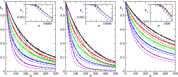
Figure 1: Average Bayes error for task 1 for two-task GP regression with kernel lengthscale $l=0.01$, noise level $\sigma^{2}=0.05$ and a fraction $\pi_{2}=0.75$ of examples for task 2. Solid lines: numerical simulations; dashed lines: approximation (7). Task correlation $\rho^{2}=0$, 0.25, 0.5, 0.75, 1 from top to bottom. Left: SE covariance function, Gaussian input distribution. Middle: SE covariance, uniform inputs. Right: OU covariance, uniform inputs. Log-log plots (insets) show tendency of asymptotic uselessness, i.e. bunching of the $\rho<1$ curves towards the one for $\rho=0$; this effect is strongest for learning of smooth functions (left and middle).

As regards the covariance function and input distribution, we analyse first the scenario studied in [21]: a squared exponential (SE) kernel $C(x,x^{\prime})=\exp[-(x-x^{\prime})^{2}/(2l^{2})]$ with lengthscale $l$, and one-dimensional inputs $x$ with a Gaussian distribution $\mathcal{N}(0,1/12)$. The kernel eigenvalues $\lambda_{i}$ are known explicitly from [22] and decay exponentially with $i$. Figure 1(left) compares numerically simulated learning curves with the predictions for $\epsilon_{1}$, the average Bayes error on task 1, from (7). Five pairs of curves are shown, for $\rho^{2}=0$, 0.25, 0.5, 0.75, 1. Note that the two extreme values represent single-task limits, where examples from task 2 are either ignored ($\rho=0$) or effectively treated as being from task 1 ($\rho=1$). Our predictions lie generally below the true learning curves, but qualitatively represent the trends well, in particular the variation with $\rho^{2}$. The curves for the different $\rho^{2}$ values are fairly evenly spaced vertically for small number of examples, $n$, corresponding to a linear dependence on $\rho^{2}$. As $n$ increases, however, the learning curves for $\rho<1$ start to bunch together and separate from the one for the fully correlated case ($\rho=1$). The approximation (7) correctly captures this behaviour, which is discussed in more detail below.

Figure 1(middle) has analogous results for the case of inputs $x$ uniformly distributed on the interval $[0,1]$; the $\lambda_{i}$ here decay exponentially with $i^{2}$ [17]. Quantitative agreement between simulations and predictions is better for this case. The discussion in [17] suggests that this is because the approximation method we have used implicitly neglects spatial variation of the dataset-averaged posterior variance $\langle V_{\tau}(x)\rangle$; but for a uniform input distribution this variation will be weak except near the ends of the input range $[0,1]$. Figure 1(right) displays similar results for an OU kernel $C(x,x^{\prime})=\exp(-|x-x^{\prime}|/l)$, showing that our predictions also work well when learning rough (nowhere differentiable) functions.

4.3 Asymptotic uselessness

The two-task results above suggest that multi-task learning is less useful asymptotically: when the number of training examples $n$ is large, the learning curves seem to bunch towards the curve for $\rho=0$, where task 2 examples are ignored, except when the two tasks are fully correlated ($\rho=1$). We now study this effect.

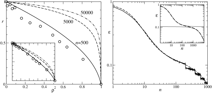
Figure 2: Left: Bayes error (parameters as in Fig. 1(left), with $n=500$) vs $\rho^{2}$. To focus on the error reduction with $\rho$, $r=[\epsilon_{1}(\rho)-\epsilon_{1}(1)]/[\epsilon_{1}(0)-\epsilon_{1}(1)]$ is shown. Circles: simulations; solid line: predictions from (7). Other lines: predictions for larger $n$, showing the approach to asymptotic uselessness in multi-task learning of smooth functions. Inset: Analogous results for rough functions (parameters as in Fig. 1(right)). Right: Learning curve for many-task learning ($T=200$, parameters otherwise as in Fig. 1(left) except $\rho^{2}=0.8$). Notice the bend around $\epsilon_{1}=1-\rho=0.106$. Solid line: simulations (steps arise because we chose to allocate examples to tasks in order $\tau=1,\ldots,T$ rather than randomly); dashed line: predictions from (7). Inset: Predictions for $T=1000$, with asymptotic forms $\epsilon=1-\rho+\rho\tilde{\epsilon}$ and $\epsilon=(1-\rho)\bar{\epsilon}$ for the two learning stages shown as solid lines.

When the number of examples for all tasks becomes large, the Bayes errors $\epsilon_{\tau}$ will become small and eventually be negligible compared to the noise variances $\sigma_{\tau}^{2}$ in (7). One then has an explicit prediction for each $\epsilon_{\tau}$, without solving $T$ self-consistency equations. If we write, for $T$ tasks, $n_{\tau}=n\pi_{\tau}$ with $\pi_{\tau}$ the fraction of examples for task $\tau$, and set $\gamma_{\tau}=\pi_{\tau}/\sigma_{\tau}^{2}$, then for large $n$

$$\epsilon_{\tau}={\textstyle\sum_{i}}\left(\lambda_{i}^{-1}\bm{D}^{-1}+n\bm{\Gamma}\right)^{-1}_{\tau\tau}={\textstyle\sum_{i}}(\bm{\Gamma}^{-1/2}[\lambda_{i}^{-1}(\bm{\Gamma}^{1/2}\bm{D}\bm{\Gamma}^{1/2})^{-1}+n\bm{I}]^{-1}\bm{\Gamma}^{-1/2})_{\tau\tau}$$ (8)

where $\bm{\Gamma}=\mbox{diag}(\gamma_{1},\ldots,\gamma_{T})$. Using an eigendecomposition of the symmetric matrix $\bm{\Gamma}^{1/2}\bm{D}\bm{\Gamma}^{1/2}=\sum_{a=1}^{T}\delta_{a}\bm{v}_{a}\bm{v}_{a}^{\mathrm{T}}$, one then shows in a few lines that (8) can be written as

$$\epsilon_{\tau}\approx\gamma_{\tau}^{-1}{\textstyle\sum_{a}}(v_{a,\tau})^{2}\delta_{a}g(n\delta_{a})$$ (9)

where $g(h)=\mathrm{tr}\,(\bm{\Lambda}^{-1}+h)^{-1}=\sum_{i}(\lambda_{i}^{-1}+h)^{-1}$ and $v_{a,\tau}$ is the $\tau$-th component of the $a$-th eigenvector $\bm{v}_{a}$. This is the general asymptotic form of our prediction for the average Bayes error for task $\tau$.

To get a more explicit result, consider the case where sample functions from the GP prior have (mean-square) derivatives up to order $r$. The kernel eigenvalues $\lambda_{i}$ then decay as $i^{-(2r+2)}$ for large $i$, and using arguments from [17] one deduces that $g(h)\sim h^{-\alpha}$ for large $h$, with $\alpha=(2r+1)/(2r+2)$. In (9) we can then write, for large $n$, $g(n\delta_{a})\approx(\delta_{a}/\gamma_{\tau})^{-\alpha}g(n\gamma_{\tau})$ and hence

$$\epsilon_{\tau}\approx g(n\gamma_{\tau})\{{\textstyle\sum_{a}}(v_{a,\tau})^{2}(\delta_{a}/\gamma_{\tau})^{1-\alpha}\}$$ (10)

When there is only a single task, $\delta_{1}=\gamma_{1}$ and this expression reduces to $\epsilon_{1}=g(n\gamma_{1})=g(n_{1}/\sigma_{1}^{2})$. Thus $g(n\gamma_{\tau})=g(n_{\tau}/\sigma_{\tau}^{2})$ is the error we would get by ignoring all examples from tasks other than $\tau$, and the term in $\{\ldots\}$ in (10) gives the “multi-task gain”, i.e. the factor by which the error is reduced because of examples from other tasks. (The absolute error reduction always vanishes trivially for $n\to\infty$, along with the errors themselves.) One observation can be made directly. Learning of very smooth functions, as defined e.g. by the SE kernel, corresponds to $r\to\infty$ and hence $\alpha\to 1$, so the multi-task gain tends to unity: multi-task learning is asymptotically useless. The only exception occurs when some of the tasks are fully correlated, because one or more of the eigenvalues $\delta_{a}$ of $\bm{\Gamma}^{1/2}\bm{D}\bm{\Gamma}^{1/2}$ will then be zero.

Fig. 2(left) shows this effect in action, plotting Bayes error against $\rho^{2}$ for the two-task setting of Fig. 1(left) with $n=500$. Our predictions capture the nonlinear dependence on $\rho^{2}$ quite well, though the effect is somewhat weaker in the simulations. For larger $n$ the predictions approach a curve that is constant for $\rho<1$, signifying negligible improvement from multi-task learning except at $\rho=1$. It is worth contrasting this with the lower bound from [21], which is linear in $\rho^{2}$. While this provides a very good approximation to the learning curves for moderate $n$ [21], our results here show that asymptotically this bound can become very loose.

When predicting rough functions, there is some asymptotic improvement to be had from multi-task learning, though again the multi-task gain is nonlinear in $\rho^{2}$: see Fig. 2(left, inset) for the OU case, which has $r=1$). A simple expression for the gain can be obtained in the limit of many tasks, to which we turn next.

4.4 Many tasks

We assume as for the two-task case that all inter-task correlations, $D_{\tau,\tau^{\prime}}$ with $\tau\neq\tau^{\prime}$, are equal to $\rho$, while $D_{\tau,\tau}=1$. This setup was used e.g. in [23], and can be interpreted as each task having a component proportional to $\sqrt{\rho}$ of a shared latent function, with an independent task-specific signal in addition. We assume for simplicity that we have the same number $n_{\tau}=n/T$ of examples for each task, and that all noise levels are the same, $\sigma_{\tau}^{2}=\sigma^{2}$. Then also all Bayes errors $\epsilon_{\tau}=\epsilon$ will be the same. Carrying out the matrix inverses in (7) explicitly, one can then write this equation as

$$\epsilon=g_{T}(n/(\sigma^{2}+\epsilon),\rho)$$ (11)

where $g_{T}(h,\rho)$ is related to the single-task function $g(h)$ from above by

$$g_{T}(h,\rho)=\frac{T-1}{T}(1-\rho)g(h(1-\rho)/T)+\left(\rho+\frac{1-\rho}{T}\right)g(h[\rho+(1-\rho)/T])$$ (12)

Now consider the limit $T\to\infty$ of many tasks. If $n$ and hence $h=n/(\sigma^{2}+\epsilon)$ is kept fixed, $g_{T}(h,\rho)\to(1-\rho)+\rho g(h\rho)$; here we have taken $g(0)=1$ which corresponds to $\mathrm{tr}\,\bm{\Lambda}=\langle C(x,x)\rangle_{x}=1$ as in the examples above. One can then deduce from (11) that the Bayes error for any task will have the form $\epsilon=(1-\rho)+\rho\tilde{\epsilon}$, where $\tilde{\epsilon}$ decays from one to zero with increasing $n$ as for a single task, but with an effective noise level $\tilde{\sigma}^{2}=(1-\rho+\sigma^{2})/\rho$. Remarkably, then, even though here $n/T\to 0$ so that for most tasks no examples have been seen, the Bayes error for each task decreases by “collective learning” to a plateau of height $1-\rho$. The remaining decay of $\epsilon$ to zero happens only once $n$ becomes of order $T$. Here one can show, by taking $T\to\infty$ at fixed $h/T$ in (12) and inserting into (11), that $\epsilon=(1-\rho)\bar{\epsilon}$ where $\bar{\epsilon}$ again decays as for a single task but with an effective number of examples $\bar{n}=n/T$ and effective noise level $\bar{\sigma}^{2}/(1-\rho)$. This final stage of learning therefore happens only when each task has seen a considerable number of exampes $n/T$. Fig. 2(right) validates these predictions against simulations, for a number of tasks ($T=200$) that is in the same ballpark as in the many-tasks application example of [24]. The inset for $T=1000$ shows clearly how the two learning curve stages separate as $T$ becomes larger.

Finally we can come back to the multi-task gain in the asymptotic stage of learning. For GP priors with sample functions with derivatives up to order $r$ as before, the function $\bar{\epsilon}$ from above will decay as $(\bar{n}/\bar{\sigma}^{2})^{-\alpha}$; since $\epsilon=(1-\rho)\bar{\epsilon}$ and $\bar{\sigma}^{2}=\sigma^{2}/(1-\rho)$, the Bayes error $\epsilon$ is then proportional to $(1-\rho)^{1-\alpha}$. This multi-task gain again approaches unity for $\rho<1$ for smooth functions ($\alpha=(2r+1)/(2r+2)\to 1$). Interestingly, for rough functions ($\alpha<1$), the multi-task gain decreases for small $\rho^{2}$ as $1-(1-\alpha)\sqrt{\rho^{2}}$ and so always lies below a linear dependence on $\rho^{2}$ initially. This shows that a linear-in-$\rho^{2}$ lower error bound cannot generally apply to $T>2$ tasks, and indeed one can verify that the derivation in [21] does not extend to this case.

5 Conclusion

We have derived an approximate prediction (7) for learning curves in multi-task GP regression, valid for arbitrary inter-task correlation matrices $\bm{D}$. This can be evaluated explicitly knowing only the kernel eigenvalues, without sampling or recourse to single-task learning curves. The approximation shows that pure transfer learning has a simple lower error bound, and provides a good qualitative account of numerically simulated learning curves. Because it can be used to study the asymptotic behaviour for large training sets, it allowed us to show that multi-task learning can become asymptotically useless: when learning smooth functions it reduces the asymptotic Bayes error only if tasks are fully correlated. For the limit of many tasks we found that, remarkably, some initial “collective learning” is possible even when most tasks have not seen examples. A much slower second learning stage then requires many examples per task. The asymptotic regime of this also showed explicitly that a lower error bound that is linear in $\rho^{2}$, the square of the inter-task correlation, is applicable only to the two-task setting $T=2$.

In future work it would be interesting to use our general result to investigate in more detail the consequences of specific choices for the inter-task correlations $\bm{D}$, e.g. to represent a lower-dimensional latent factor structure. One could also try to deploy similar approximation methods to study the case of model mismatch, where the inter-task correlations $\bm{D}$ would have to be learned from data. More challenging, but worthwhile, would be an extension to multi-task covariance functions where task and input-space correlations to not factorize.

References

- [1] C K I Williams and C Rasmussen. Gaussian Processes for Machine Learning. MIT Press, Cambridge, MA, 2006.
- [2] J Baxter. A model of inductive bias learning. J. Artif. Intell. Res., 12:149–198, 2000.
- [3] S Ben-David and R S Borbely. A notion of task relatedness yielding provable multiple-task learning guarantees. Mach. Learn., 73(3):273–287, December 2008.
- [4] Y W Teh, M Seeger, and M I Jordan. Semiparametric latent factor models. In Workshop on Artificial Intelligence and Statistics 10, pages 333–340. Society for Artificial Intelligence and Statistics, 2005.
- [5] E V Bonilla, F V Agakov, and C K I Williams. Kernel multi-task learning using task-specific features. In Proceedings of the 11th International Conference on Artificial Intelligence and Statistics (AISTATS). Omni Press, 2007.
- [6] E V Bonilla, K M A Chai, and C K I Williams. Multi-task Gaussian process prediction. In J C Platt, D Koller, Y Singer, and S Roweis, editors, NIPS 20, pages 153–160, Cambridge, MA, 2008. MIT Press.
- [7] M Alvarez and N D Lawrence. Sparse convolved Gaussian processes for multi-output regression. In D Koller, D Schuurmans, Y Bengio, and L Bottou, editors, NIPS 21, pages 57–64, Cambridge, MA, 2009. MIT Press.
- [8] G Leen, J Peltonen, and S Kaski. Focused multi-task learning using Gaussian processes. In Dimitrios Gunopulos, Thomas Hofmann, Donato Malerba, and Michalis Vazirgiannis, editors, Machine Learning and Knowledge Discovery in Databases, volume 6912 of Lecture Notes in Computer Science, pages 310–325. Springer Berlin, Heidelberg, 2011.
- [9] M A Álvarez, L Rosasco, and N D Lawrence. Kernels for vector-valued functions: a review. Foundations and Trends in Machine Learning, 4:195–266, 2012.
- [10] A Maurer. Bounds for linear multi-task learning. J. Mach. Learn. Res., 7:117–139, 2006.
- [11] M Opper and F Vivarelli. General bounds on Bayes errors for regression with Gaussian processes. In M Kearns, S A Solla, and D Cohn, editors, NIPS 11, pages 302–308, Cambridge, MA, 1999. MIT Press.
- [12] G F Trecate, C K I Williams, and M Opper. Finite-dimensional approximation of Gaussian processes. In M Kearns, S A Solla, and D Cohn, editors, NIPS 11, pages 218–224, Cambridge, MA, 1999. MIT Press.
- [13] P Sollich. Learning curves for Gaussian processes. In M S Kearns, S A Solla, and D A Cohn, editors, NIPS 11, pages 344–350, Cambridge, MA, 1999. MIT Press.
- [14] D Malzahn and M Opper. Learning curves for Gaussian processes regression: A framework for good approximations. In T K Leen, T G Dietterich, and V Tresp, editors, NIPS 13, pages 273–279, Cambridge, MA, 2001. MIT Press.
- [15] D Malzahn and M Opper. A variational approach to learning curves. In T G Dietterich, S Becker, and Z Ghahramani, editors, NIPS 14, pages 463–469, Cambridge, MA, 2002. MIT Press.
- [16] D Malzahn and M Opper. Statistical mechanics of learning: a variational approach for real data. Phys. Rev. Lett., 89:108302, 2002.
- [17] P Sollich and A Halees. Learning curves for Gaussian process regression: approximations and bounds. Neural Comput., 14(6):1393–1428, 2002.
- [18] P Sollich. Gaussian process regression with mismatched models. In T G Dietterich, S Becker, and Z Ghahramani, editors, NIPS 14, pages 519–526, Cambridge, MA, 2002. MIT Press.
- [19] P Sollich. Can Gaussian process regression be made robust against model mismatch? In Deterministic and Statistical Methods in Machine Learning, volume 3635 of Lecture Notes in Artificial Intelligence, pages 199–210. Springer Berlin, Heidelberg, 2005.
- [20] M Urry and P Sollich. Exact larning curves for Gaussian process regression on large random graphs. In J Lafferty, C K I Williams, J Shawe-Taylor, R S Zemel, and A Culotta, editors, NIPS 23, pages 2316–2324, Cambridge, MA, 2010. MIT Press.
- [21] K M A Chai. Generalization errors and learning curves for regression with multi-task Gaussian processes. In Y Bengio, D Schuurmans, J Lafferty, C K I Williams, and A Culotta, editors, NIPS 22, pages 279–287, 2009.
- [22] H Zhu, C K I Williams, R J Rohwer, and M Morciniec. Gaussian regression and optimal finite dimensional linear models. In C M Bishop, editor, Neural Networks and Machine Learning. Springer, 1998.
- [23] E Rodner and J Denzler. One-shot learning of object categories using dependent Gaussian processes. In Michael Goesele, Stefan Roth, Arjan Kuijper, Bernt Schiele, and Konrad Schindler, editors, Pattern Recognition, volume 6376 of Lecture Notes in Computer Science, pages 232–241. Springer Berlin, Heidelberg, 2010.
- [24] T Heskes. Solving a huge number of similar tasks: a combination of multi-task learning and a hierarchical Bayesian approach. In Proceedings of the Fifteenth International Conference on Machine Learning (ICML’98), pages 233–241. Morgan Kaufmann, 1998.