Discussion: Latent variable graphical model selection via convex optimization

10.1214/11-AOS949

T1Supported in part by NSF Career Award DMS-08-46234.

I want to start by congratulating Professors Chandrasekaran, Parrilo and Willsky for this fine piece of work. Their paper, hereafter referred to as CPW, addresses one of the biggest practical challenges of Gaussian graphical models—how to make inferences for a graphical model in the presence of missing variables. The difficulty comes from the fact that the validity of conditional independence relationships implied by a graphical model relies critically on the assumption that all conditional variables are observed, which of course can be unrealistic. As CPW shows, this is not as hopeless as it might appear to be. They characterize conditions under which a conditional graphical model can be identified, and offer a penalized likelihood method to reconstruct it. CPW notes that with missing variables, the concentration matrix of the observables can be expressed as the difference between a sparse matrix and a low-rank matrix; and suggests to exploit the sparsity using an $\ell_{1}$ penalty and the low-rank structure by a trace norm penalty. In particular, the trace norm penalty or, more generally, nuclear norm penalties, can be viewed as a convex relaxation to the more direct rank constraint. Its use oftentimes comes as a necessity because rank constrained optimization could be computationally prohibitive. Interestingly, as I note here, the current problem actually lends itself to efficient algorithms in dealing with the rank constraint, and therefore allows for an attractive alternative to the approach of CPW.

1 Rank constrained latent variable graphical Lasso

Recall that the penalized likelihood estimate of CPW is defined as

$$(\hat{S}_{n},\hat{L}_{n})=\mathop{\operatorname{arg\,min}}_{L\succeq 0,S-L\succ 0}\bigl{\{}-\ell(S-L,\Sigma_{O}^{n})+\lambda_{n}\bigl{(}\gamma\|S\|_{1}+\operatorname{trace}(L)\bigr{)}\bigr{\}},$$

where the vector $\ell_{1}$ norm and trace/nuclear norm penalties are designated to induce sparsity among elements of $S$ and low-rank structure of $L$ respectively. Of course, we can attempt a more direct rank penalty as opposed to the nuclear norm penalty on $L$, leading to

$$(\hat{S}_{n},\hat{L}_{n})=\mathop{\operatorname{arg\,min}}_{L\succeq 0,S-L\succ 0}\bigl{\{}-\ell(S-L,\Sigma_{O}^{n})+\lambda_{n}\bigl{(}\gamma\|S\|_{1}+\operatorname{rank}(L)\bigr{)}\bigr{\}};$$

or for computational purposes, it is more convenient to consider the constrained version:

$$(\hskip 1.0pt\hat{\vphantom{\rule{1.0pt}{6.14584pt}}\smash{\hat{S}}}_{n},\hskip 1.0pt\hat{\vphantom{\rule{1.0pt}{6.14584pt}}\smash{\hat{L}}}_{n})=\mathop{\mathop{\operatorname{arg\,min}}_{L\succeq 0,S-L\succ 0}}_{\operatorname{rank}(L)\leq r}\{-\ell(S-L,\Sigma_{O}^{n})+\lambda_{n}\|S^{\dagger}\|_{1}\},$$

for some integer $0\leq r\leq p$, where $S^{\dagger}=S-{\rm diag}(S)$, that is, $S^{\dagger}$ equals $S$ except that its diagonals are replaced by $0$. This slight modification reflects our intention to encourage sparsity on the off-diagonal entries of $S$ only. The remaining discussion, however, can be easily adapted to deal with the original vector $\ell_{1}$ penalty on $S$. It is clear that when $r=0$, that is, $L=0$, this new estimator reduces to the so-called graphical Lasso estimate (glasso, for short) of Yuan and Lin (2007). See also Banerjee, El Ghaoui and d’Aspremont (2008), Friedman, Hastie and Tibshirani (2008), and Rothman et al. (2008). Drawn to this similarity, I shall hereafter refer to this method as the latent variable graphical Lasso, or LVglasso, for short.

Common wisdom on $(\hskip 1.0pt\hat{\vphantom{\rule{1.0pt}{6.14584pt}}\smash{\hat{S}}}_{n},\hskip 1.0pt\hat{\vphantom{\rule{1.0pt}{6.14584pt}}\smash{\hat{L}}}_{n})$ is that it is infeasible to compute because of the nonconvexity of the rank constraint. Interestingly, though, this more direct approach actually allows for fast computation, thanks to a combination of EM algorithm and some recent advances in computing graphical Lasso estimates for high-dimensional problems.

2 An EM algorithm

The constraint $\operatorname{rank}(L)\leq r$ amounts to postulating $r$ latent variables. The latent variable model naturally has a missing data formulation. It is clear that when observing the complete data $X=(X_{O}^{\sf T},X_{H}^{\sf T})^{\sf T}$, the LVglasso estimator becomes

$$\hat{K}_{\lambda}=\mathop{\operatorname{arg\,min}}_{K\in\mathbb{R}^{(p+r)\times(p+r)},K\succ 0}\{L(K)+\lambda\|K_{O}^{\dagger}\|_{1}\},$$

where

$$L(K)=-\ln\det(K)+\operatorname{trace}\bigl{(}\Sigma_{(OH)}^{n}K\bigr{)}$$

and $\Sigma_{(OH)}^{n}$ is the sample covariance matrix of the full data. Now that $X_{H}$ is unobservable, we can use an EM algorithm which iteratively applies the following two steps:

Calculate the expected value of the penalized negative log-likelihood function, with respect to the conditional distribution of $X_{H}$ given $X_{O}$ under the current estimate $K^{(t)}$ of $K$, leading to the so-called Q function:

$$Q\bigl{(}K|K^{(t)}\bigr{)} = \mathbb{E}_{X_{H}|X_{O},K^{(t)}}[L(K)+\lambda\|K_{O}^{\dagger}\|_{1}]$$

$$= -\ln\det(K)+\operatorname{trace}\bigl{\{}\mathbb{E}_{X_{H}|X_{O},K^{(t)}}\bigl{(}\Sigma_{(OH)}^{n}\bigr{)}K\bigr{\}}+\lambda\|K_{O}^{\dagger}\|_{1}.$$

Recall that $X_{H}|X_{O},K^{(t)}$ follows a normal distribution with

$$\mathbb{E}\bigl{(}X_{H}|X_{O},K^{(t)}\bigr{)}=\Sigma^{(t)}_{HO}\bigl{(}\Sigma^{(t)}_{O}\bigr{)}^{-1}X_{O}$$

and

$$\operatorname{Var}\bigl{(}X_{H}|X_{O},K^{(t)}\bigr{)}=\Sigma^{(t)}_{H}-\Sigma^{(t)}_{HO}\bigl{(}\Sigma^{(t)}_{O}\bigr{)}^{-1}\Sigma^{(t)}_{OH},$$

where $\Sigma^{(t)}=(K^{(t)})^{-1}$. Therefore,

$$\mathbb{E}_{X_{H}|X_{O},K^{(t)}}(\Sigma_{OH}^{n})=\Sigma^{n}_{O}\bigl{(}\Sigma^{(t)}_{O}\bigr{)}^{-1}\Sigma^{(t)}_{oH}$$

and

$$\mathbb{E}_{X_{H}|X_{O},K^{(t)}}(\Sigma_{H}^{n})=\Sigma^{(t)}_{H}-\Sigma^{(t)}_{HO}\bigl{(}\Sigma^{(t)}_{O}\bigr{)}^{-1}\Sigma^{(t)}_{OH}+\Sigma^{(t)}_{HO}\bigl{(}\Sigma^{(t)}_{O}\bigr{)}^{-1}\Sigma^{n}_{O}\bigl{(}\Sigma^{(t)}_{O}\bigr{)}^{-1}\Sigma^{(t)}_{OH}.$$

Maximize $Q(\cdot|K^{(t)})$ over all $(p+r)\times(p+r)$ positive definite matrices. We first note that if we replace the penalty term $\|K_{O}^{\dagger}\|_{1}$ with $\|K^{\dagger}\|_{1}$, then maximizing $Q(\cdot|K^{(t)})$ becomes a glasso problem:

$$\max_{K\in\mathbb{R}^{(p+r)\times(p+r)},K\succ 0}\bigl{\{}-\ln\det(K)+\operatorname{trace}\{WK\}+\lambda\|K^{\dagger}\|_{1}\bigr{\}},$$

where $W=\mathbb{E}_{X_{H}|X_{O},K^{(t)}}(\Sigma_{(OH)}^{n})$. As shown in Banerjee, El Ghaoui andd’Aspremont (2008), Friedman, Hastie and Tibshirani (2008) and Yuan (2008), this problem can be solved iteratively. At each iteration, one row and, correspondingly, one column of $K$, due to symmetry, are updated by solving a Lasso problem. The same idea can be applied here to maximize $Q(\cdot|K^{(t)})$. The only difference is that in each of the Lasso problems, we leave the coordinates corresponding to the latent variables unpenalized. This extension has

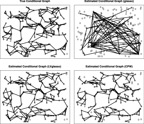
Figure 1: True graphical model and its estimates.

been implemented in the R package glasso [Friedman, Hastie and Tibshirani (2008)].

3 Example

For illustration purposes, I conducted a simple numerical experiment. In this experiment the interest was in recovering a $p=198$ dimensional graphical model with $h=2$ missing variables. The graphical model was generated in a similar fashion as that from Meinshausen and Bühlmann (2006). I first simulated 198 locations uniformly over a square.

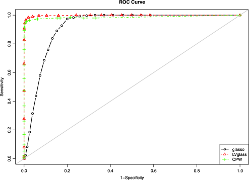
Figure 2: Accuracy of reconstructed conditional graphical model.

Between each pair of locations, I put an edge with probability $2\phi(d\sqrt{p})$, where $\phi(\cdot)$ is the density function of the standard normal distribution and $d$ is the distance between the two locations, unless one of the locations is already connected with four other locations. The two hidden variables were connected with all $p$ observed variables. The entries of the inverse covariance matrix corresponding to the edges between the observables were assigned with value $0.2$, between the observables and the latent variables were assigned with a uniform random value between 0 and $0.12$, to ensure the positive definiteness. A typical simulated graphical model among the 198 observed variables conditional on the two latent variables is given in the top left panel of Figure 1. We apply both the method of CPW and LVglasso, along with glasso, to the data. We used the MATLAB code provided by CPW to compute their estimates. As observed by CPW, their estimate typically is insensitive to a wide range of values of $\gamma$, and we report here the results with the default choice of $\gamma=5$ without loss of generality. Similarly, for LVglasso, little variation was observed for $r=2,\ldots,10$, and we shall focus on $r=2$ for brevity. The choice of $\lambda$ plays a critical role for both methods. We compute both estimators for a fine grid of $\lambda$. With the main focus on recovering the conditional graphical model, that is, the sparsity pattern of $S$, we report in Figure 2 the ROC curve for both methods. For contrast, we also reported the result for glasso which neglects the missingness. In Figure 1, we also presented the estimated graphical model for each method that is closest to the truth. These results clearly demonstrate the necessity of accounting for the latent variables. It is also interesting to note that the rank constrained estimator performs slightly better in this example over the trace norm penalization method of CPW.

The preliminary results presented here suggest that direct rank constraint may provide a competitive alternative to the trace norm penalization for recovering graphical models with latent variables. It is of interest to investigate more rigorously how the two methods compare with each other.

References

- Banerjee, El Ghaoui and d’Aspremont (2008) {barticle}[mr] \bauthor\bsnmBanerjee, \bfnmOnureena\binitsO., \bauthor\bsnmEl Ghaoui, \bfnmLaurent\binitsL. and \bauthor\bsnmd’Aspremont, \bfnmAlexandre\binitsA. (\byear2008). \btitleModel selection through sparse maximum likelihood estimation for multivariate Gaussian or binary data. \bjournalJ. Mach. Learn. Res. \bvolume9 \bpages485–516. \bidissn=1532-4435, mr=2417243 \bptokimsref \endbibitem
- Friedman, Hastie and Tibshirani (2008) {barticle}[auto:STB—2012/05/30—10:51:56] \bauthor\bsnmFriedman, \bfnmJ.\binitsJ., \bauthor\bsnmHastie, \bfnmT.\binitsT. and \bauthor\bsnmTibshirani, \bfnmT.\binitsT. (\byear2008). \btitleSparse inverse covariance estimation with the graphical lasso. \bjournalBiostatistics \bvolume9 \bpages432–441. \bptokimsref \endbibitem
- Meinshausen and Bühlmann (2006) {barticle}[mr] \bauthor\bsnmMeinshausen, \bfnmNicolai\binitsN. and \bauthor\bsnmBühlmann, \bfnmPeter\binitsP. (\byear2006). \btitleHigh-dimensional graphs and variable selection with the lasso. \bjournalAnn. Statist. \bvolume34 \bpages1436–1462. \biddoi=10.1214/009053606000000281, issn=0090-5364, mr=2278363 \bptokimsref \endbibitem
- Rothman et al. (2008) {barticle}[mr] \bauthor\bsnmRothman, \bfnmAdam J.\binitsA. J., \bauthor\bsnmBickel, \bfnmPeter J.\binitsP. J., \bauthor\bsnmLevina, \bfnmElizaveta\binitsE. and \bauthor\bsnmZhu, \bfnmJi\binitsJ. (\byear2008). \btitleSparse permutation invariant covariance estimation. \bjournalElectron. J. Stat. \bvolume2 \bpages494–515. \biddoi=10.1214/08-EJS176, issn=1935-7524, mr=2417391 \bptokimsref \endbibitem
- Yuan (2008) {barticle}[mr] \bauthor\bsnmYuan, \bfnmMing\binitsM. (\byear2008). \btitleEfficient computation of regularized estimates in Gaussian graphical models. \bjournalJ. Comput. Graph. Statist. \bvolume17 \bpages809–826. \biddoi=10.1198/106186008X382692, issn=1061-8600, mr=2649068 \bptokimsref \endbibitem
- Yuan and Lin (2007) {barticle}[mr] \bauthor\bsnmYuan, \bfnmMing\binitsM. and \bauthor\bsnmLin, \bfnmYi\binitsY. (\byear2007). \btitleModel selection and estimation in the Gaussian graphical model. \bjournalBiometrika \bvolume94 \bpages19–35. \biddoi=10.1093/biomet/asm018, issn=0006-3444, mr=2367824 \bptokimsref \endbibitem