Heat exchanges in a quenched ferromagnet

Abstract

The off-equilibrium probability distribution of the heat exchanged by a ferromagnet in a time interval after a quench below the critical point is calculated analytically in the large-$N$ limit. The distribution is characterized by a singular threshold $Q_{C}<0$, below which a macroscopic fraction of heat is released by the $k=0$ Fourier component of the order parameter. The mathematical structure producing this phenomenon is the same responsible of the order parameter condensation in the equilibrium low temperature phase. The heat exchanged by the individual Fourier modes follows a non trivial pattern, with the unstable modes at small wave vectors warming up the modes around a characteristic finite wave vector $k_{M}$. Two internal temperatures, associated to the $k=0$ and $k=k_{M}$ modes, rule the heat currents through a fluctuation relation similar to the one for stationary systems in contact with two thermal reservoirs.

Finding the principles underlying the probability measures of non-equilibrium fluctuations is one of the most challenging and far reaching open questions in modern statistical physics. Large deviation theory, as recognized in the last years, gives a general theoretical framework for describing probability distribution functions (PDF) in non-equilibrium states touchette . However, in spite of recent important developments Jona , explicit calculations, especially for interacting systems, are limited to few cases touchette . A major advance for non-equilibrium stationary states has been the recognition of a general symmetry of the PDF of certain observables, described by the so-called fluctuation theorems FL1 ; FL2 . For example, for a system in contact with reservoirs at two inverse temperatures $\beta_{1}<\beta_{2}$ FL3 ; FL4 , the probability distribution $P(Q)$ that the heat $Q$ flows from the first to the second heat bath in a large time interval is related to $P(-Q)$ by

$$\ln\frac{P(Q)}{P(-Q)}=(\beta_{2}-\beta_{1}){Q}.$$ (1)

Fluctuation behavior in non-stationary states is by far less understood. In the thoroughly investigated field of aging systems, such as quenched ferromagnets or binary mixtures, disordered materials and glasses, heat PDF have been considered only numerically in some specific disordered models crisrit and, recently, in an experiment for a brownian particle peliti trapped in an aging bath ciliberto . Understanding the properties of heat fluxes in these systems is of great importance also for what concerns the notion of an effective temperature KC , which is expected to regulate such fluxes similarly to what the ordinary temperature does in equilibrium.

In this Letter we address the latter category of problems, by studying the probability distribution of heat exchanges in a ferromagnetic model quenched from a disordered state to a final temperature below the critical point. We do this by an exact calculation carried out on the time dependent Ginzburg-Landau model with an $N$-component vector order parameter in the large-$N$ limit bray . Specifically, we find the analytical form of the probability distribution $P(Q,t,t_{w})$, where $Q$ is the heat exchanged during the time interval $[t_{w},t]$ following the quench. Most interesting is the existence of a singular threshold $Q_{C}$, such that for $Q<Q_{C}$ the macroscopic amount of heat $Q-Q_{C}$ is entirely released by the zero wave vector mode. This comes about through the same mechanism responsible of the transition to the low temperature phase in the equilibrium version of the model berlkac ; condvs . Furthermore, we find that $P(Q,t,t_{w})$ asymptotically obeys a fluctuation relation akin to Eq. (1), even though the system is not in a stationary state. This can be interpreted as due to the heat exchanged between the condensing $k=0$ mode, lowering the system energy as an effect of the ordering process, and the modes at some finite characteristic wave vector $k_{M}$. The two inverse temperatures playing the role of $\beta_{1},\beta_{2}$ in Eq. (1) arise as the typical energy scales associated to these two kinds of non-equilibrium modes, and reduce to the bath temperature when the system is in equilibrium.

We consider a system of volume $V$, described by the Ginzburg-Landau Hamiltonian

$$H[\boldsymbol{\varphi}]=\int_{V}d^{d}x\left[\frac{1}{2}(\nabla\boldsymbol{\varphi})^{2}+\frac{r}{2}\boldsymbol{\varphi}^{2}+\frac{g}{4N}\left(\boldsymbol{\varphi}^{2}\right)^{2}\right]$$ (2)

where $r<0$, $g>0$, and $\boldsymbol{\varphi}=(\varphi_{1},..,\varphi_{N})$, is the $N$-component order parameter field. Dynamics is governed by the Langevin equation

$$\partial\varphi_{\alpha}/\partial t=-\delta H[\boldsymbol{\varphi}]/\delta\varphi_{\alpha}+\eta_{\alpha},$$ (3)

where $\varphi_{\alpha},\eta_{\alpha}$ stand for $\varphi_{\alpha}(\boldsymbol{x},t),\eta_{\alpha}(\boldsymbol{x},t)$ and the latter one represents the Gaussian white noise generated by the thermal bath with averages $<\eta_{\alpha}(\boldsymbol{x},t)>=0$ and $<\eta_{\alpha}(\boldsymbol{x},t)\eta_{\beta}(\boldsymbol{x^{\prime}},t^{\prime})>=2T\delta_{\alpha\beta}\delta(t-t^{\prime})\delta(\vec{x}-\vec{x}^{\prime})$. The leading order of all quantities of interest in the $1/N$-expansion can be obtained by replacing the above Hamiltonian with the time-dependent effective one

$${\cal H}[\boldsymbol{\varphi}]=\frac{1}{2}\int_{V}d^{d}x\left[(\nabla\boldsymbol{\varphi})^{2}+(r+gS(t))\boldsymbol{\varphi}^{2}\right]-(NVg/4)S^{2}(t)$$ (4)

where $S(t)=\langle\boldsymbol{\varphi}^{2}(\boldsymbol{x},t)\rangle/N$ must be computed self-consistently and angular brackets stand for the average over both initial condition and thermal noise. Due to space homogeneity, the quantity $S$ only depends on time. The remarkable feature of the large-$N$ limit is that the dynamics generated by ${\cal H}$, although retaining all the relevant features of the phase-ordering process, becomes exactly soluble coniglio ; bray . By Fourier transformation one obtains a decoupled set of formally linear equations of motion

$$\frac{\partial}{\partial t}\varphi_{\alpha}(\boldsymbol{k},t)=-\omega(k,t)\varphi_{\alpha}(\boldsymbol{k},t)+\eta_{\alpha}(\boldsymbol{k},t)$$ (5)

where the stiffness of each mode is given by $\omega(k,t)=k^{2}+r+gS(t)$ and $<\eta_{\alpha}(\boldsymbol{k},t)>=0$, $<\eta_{\alpha}(\boldsymbol{k},t)\eta_{\beta}(\boldsymbol{k}^{\prime},t^{\prime})>=2T\delta_{\alpha\beta}\delta(\boldsymbol{k}+\boldsymbol{k}^{\prime})\delta(t-t^{\prime})$. Integrating Eq. (5) and taking averages, the various observables can be obtained noi2002 . In particular, the two-times structure factor $C(k,t,t_{w})=(1/V)\langle\varphi_{\alpha}(\boldsymbol{k},t)\varphi_{\alpha}(-\boldsymbol{k},t_{w})\rangle$ with $t_{w}\leq t$ will play a relevant role in the following.

The probability to release the heat $Q$ per component in the time interval $[t_{w},t]$ is defined by

$$P(Q;t_{w},t)=\int d[\boldsymbol{\varphi}_{t}]d[\boldsymbol{\varphi}_{w}]{\cal P}(\boldsymbol{\varphi}_{t},\boldsymbol{\varphi}_{w})\delta(Q-\frac{{\cal H}[\boldsymbol{\varphi}_{t}]}{N}+\frac{{\cal H}[\boldsymbol{\varphi}_{w}]}{N}),$$ (6)

where ${\cal P}(\boldsymbol{\varphi}_{t},\boldsymbol{\varphi}_{w})=\prod_{k,\alpha}{\cal P}_{k,\alpha}(\varphi_{\alpha}(\boldsymbol{k},t),\varphi_{\alpha}(\boldsymbol{k},t_{w}))$ is the joint probability of the two configurations $(\boldsymbol{\varphi}_{t},\boldsymbol{\varphi}_{w})$ at the times $t$ and $t_{w}$. For a Gaussian process

$${\cal P}_{k,\alpha}(\varphi_{\alpha,t},\varphi_{\alpha,w})={\cal N}^{-1}\exp\left\{-\frac{C_{tt}C_{ww}}{2V(C_{tt}C_{ww}-C^{2}_{wt})}\left[\frac{\varphi^{2}_{\alpha,t}}{C_{tt}}+\frac{\varphi^{2}_{\alpha,w}}{C_{ww}}-\frac{2C_{wt}\varphi_{\alpha,t}\varphi_{\alpha,w}}{C_{tt}C_{ww}}\right]\right\}$$ (7)

where the short notation $C_{wt}\equiv C(k,t,t_{w})$ (and similarly for $C_{tt},C_{ww}$) has been introduced and ${\cal N}$ is the normalization. Next, using the representation $\delta(x)=\frac{1}{2\pi i}\int_{-i\infty}^{i\infty}e^{-zx}dz$ of the Dirac $\delta$-function and carrying out the integration in Eq. (6), we find

$$P(Q;t,t_{w})=\int_{z_{0}-i\infty}^{z_{0}+i\infty}\frac{dz}{2\pi i}\,e^{Vh({\cal Q},z;t,t_{w})}$$ (8)

where ${\cal Q}=\frac{Q}{V}$ is the heat density and the real quantity $z_{0}$ is chosen in such a way that the integral is well defined berlkac . For large $V$ discrete sums over wave vectors can be replaced by integrals, yielding

$$h({\cal Q};z;t,t_{w})=-z[{\cal Q}+gU(t,t_{w})]-(1/2)\int_{\Lambda}\frac{d^{d}k}{(2\pi)^{d}}\ln[1-zq(k,t,t_{w})-z^{2}b(k,t,t_{w})]$$ (9)

where

$$U(t,t_{w})=[S^{2}(t)-S^{2}(t_{w})]/4,$$ (10)

$$b(k,t,t_{w})=\omega(k,t)\omega(k,t_{w})[C(k,t,t)C(k,t_{w},t_{w})-C^{2}(k,t,t_{w})],$$ (11)

$$q(k,t,t_{w})=\omega(k,t)C(k,t,t)-\omega(k,t_{w})C(k,t_{w},t_{w}),$$ (12)

and the symbol $\int_{\Lambda}$ denotes an integral with an ultraviolet cut-off $\Lambda$ related to the lattice spacing.

Eqs. (8,9) are completely general. Different dynamical protocols are encoded into the correlation $C$. We start our analysis from the simpler case in which the system is in equilibrium at a generic temperature $T$. In this case $\omega(k,t)=\omega_{eq}(k)$ and $C(k,t,t)=C_{eq}(k)$ do not depend on time due to stationarity, so from Eq. (12) $q=0$ and similarly $U=0$. Moreover $C(k,t,t_{w})=C_{eq}(k,t-t_{w})=(T/\omega_{eq})\exp[-\omega_{eq}(t-t_{w})]$ noi2002 , hence $b=T^{2}[1-\exp[-2\omega_{eq}(t-t_{w})]$. In the large $V$ limit, the integral in (8) can be computed by the steepest descent method. The saddle point equation ${\frac{dh}{dz}\vline}_{z=z^{*}}=0$ reads

$${\cal Q}=\int_{\Lambda}\frac{d^{d}k}{(2\pi)^{d}}\frac{z^{*}(t,t_{w})b(k,t,t_{w})}{1-{z^{*}(t,t_{w})}^{2}b(k,t,t_{w})}.$$ (13)

In order for $h$ in Eq. (9) to be defined, it must be $z\neq b(k,t,t_{w})^{-1/2}$ $\forall k,t,t_{w}$. This, for $t-t_{w}\gg 1/\omega_{eq}(\Lambda)$, requires $-\beta<z_{0}<\beta$, with $\beta=1/T$. From the above expression of $b$ one sees that the integral approaches infinity as $z^{*}\to\pm\beta$ so that Eq.(13) admits a real solution $z^{*}$ for any value of ${\cal Q}$. The large deviation function defined by

$$P(Q;t,t_{w})=\exp\{V{\cal L}({\cal Q};t,t_{w})\}$$ (14)

is given by ${\cal L}({\cal Q};t,t_{w})=h({\cal Q};z^{*};t-t_{w})$ and is plotted in the inset of Fig. 1. It is symmetric and, for ${\cal Q}$ not too small behaves linearly, ${\cal L}\simeq-\beta|{\cal Q}|$, since $z^{*}$ rapidly converges to $\beta$ as ${\cal Q}$ increases. Notice that the equilibrium temperature can be read out from the singular points of $h$, which in turn regulate the exponential decay of the tails of $P$.

Next, we consider the quench from infinite temperature to $T<T_{c}$, starting with $T=0$. Since $q(k,t,t_{w})$ will now play a central role, let us comment on its physical meaning. Using the normal modes decomposition, the average energy at the time $t$ can be written as $\langle{\cal H}\rangle=\frac{N}{2}\sum_{\boldsymbol{k}}\omega(k,t)C(k,t,t)-(NVg/4)S^{2}(t)$. This shows that $q$ in Eq. (12) can be interpreted as the average heat (per component) exchanged by the individual modes, since the contributions due to $VgS^{2}/4$ become negligible at large times as we will show below.

In a zero temperature quench, one has $C(k,t,t_{w})=\sqrt{C(k,t,t)C(k,t_{w},t_{w})}$, which implies $b=0$. In what follows we will consider the large $t_{w}$ limit. In this regimes one finds bray ; coniglio ; noi2002 $S(t)=-r/g-d/(4gt)$ and the dynamical scaling property ${L(t_{w})^{-d}C(k,t,t_{w})}=C(x,y)$, where $x=t/t_{w}$, $y=kt_{w}^{1/2}$, $L(t_{w})=(2t_{w})^{1/2}$ is the characteristic lengthscale at the age $t_{w}$ of the system, and $C(x,y)=(4\pi)^{d/2}(-r/g)x^{d/4}\exp[-y^{2}(x+1)]$. Hence, using these results, also $q$ can be written in the scaling form

$$\frac{q(y,x)}{q_{typ}}=(xy^{2}-\frac{d}{4})x^{\frac{d}{2}-1}e^{-2xy^{2}}-(y^{2}-\frac{d}{4})e^{-2y^{2}}$$ (15)

where $q_{typ}(t_{w})=-[r(8\pi)^{\frac{d}{2}}t_{w}^{d/2-1}/g]$ is the typical age-dependent scale of heat fluxes. Notice that, for fixed $x$ and $y$, $q$ grows like $t_{w}^{d/2-1}$. Therefore, using the expression of $S$ given above, the extra term $(NVg/4)[S^{2}(t)-S^{2}(t_{w})]\propto(t_{w}^{-1}-t^{-1})\propto t_{w}^{-1}(1-x^{-1})$ is negligible with respect to $q$, as anticipated. The quantity $q$ is plotted in Fig. 2 against $y$ for two different values of $x$. For any $x$ there is a negative minimum $-\beta_{0}^{-1}\equiv q(x,0)$ at the origin. Since $q$ is the average heat exchanged by the single modes, this means that the components around $k=0$ cool as the time goes on and that the cooling increases with the time difference, as intuitively expected. However, the shape of the curves shows that the rate of cooling decreases as $y$ increases, with the unexpected and quite interesting feature of the development of a positive peak $\beta_{M}^{-1}\equiv q(x,y_{M})$, which is more pronounced for the larger time differences. This implies that the modes under the positive peak warm up as time goes on. Since the thermal bath is at zero temperature, this extra heat can only originate in the heat redistribution due to the coupling among the modes. In fact, it should be kept in mind that the linearization of the equations of motion is only formal, the nonlinearity having been preserved through the mean field term $S(t)$. For yet larger values of $y$ the curves become flat about zero, indicating that the large $k$ modes are equilibrated.

In order to see what are the implications of the above features on the properties of $P(Q;t,t_{w})$, let us compute the integral in (8). Recalling that $b=0$, for $h$ in Eq. (9) to be defined, it must be $z\neq q(k,t,t_{w})^{-1}$ $\forall k,t,t_{w}$. With the form (15) of $q$ (see Fig. 2) this translates into $-\beta_{0}<z_{0}<\beta_{M}$. The analyticity domain of $h$ is shown in the inset of Fig. 2. Notice that, in this far from equilibrium situation, $\beta_{0}$ and $\beta_{M}$ play a role analogous to that of the inverse bath temperature $\beta$ in equilibrium. We now compute the integral in Eq. (8) by steepest descent. The saddle point $z^{*}$, if it exists, must satisfy the above constraint and the saddle point equation ${\cal Q}=G(z;t,t_{w})|_{z=z^{*}(t,t_{w})}$, with

$$G(z;t,t_{w})=\frac{1}{2}\int_{\Lambda}\frac{d^{d}k}{(2\pi)^{d}}\frac{q(k,t,t_{w})}{1-zq(k,t,t_{w})}-gU(t,t_{w}).$$ (16)

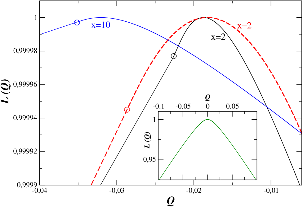
Figure 1: The large deviation function ${\cal L}({\cal Q};t,t_{w})$ is plotted against ${\cal Q}$, in $d=3$, for $t_{w}=10$ and two values of $x$ for a quench to $T=0$ (continuous lines), or $T\approx T_{c}/3$ (dashed line). Circles represent ${\cal Q}_{c}$. In the inset the same quantity is plotted in equilibrium at $T<T_{c}$.

Restricting the analysis to $2<d<4$ and using Eq. (15), one finds that $G(z=-\beta_{0})\equiv{\cal Q}_{c}<0$ is finite, while $G$ approaches infinity as $z$ tends to $\beta_{M}$. Therefore now the saddle point equation admits a solution only for ${\cal Q}>{\cal Q}_{c}$, and the integration path is shown in the inset of Fig. 2. Instead, for ${\cal Q}\leq{\cal Q}_{c}$, exploiting the analyticity of $h$ in the neighborhood of the branch point $z=-\beta_{0}$, an analysis similar to the classical one of berlkac shows that the steepest descent route deforms into a cusp whose peak is sticked in $z=-\beta_{0}$ (see inset of Fig. (2)). With this saddle point structure, finally one obtains

$$2\pi P(Q;t,t_{w})=\exp[Vh({\cal Q};z_{steep};t,t_{w})]\,,\qquad z_{steep}\,=\,\left\{\,\begin{array}[]{ccl}z^{*}({\cal Q};t,t_{w})\quad\mbox{for}\quad{\cal Q}>{\cal Q}_{c}\\ -\beta_{0}\qquad\quad\,\,\,\,\,\,\mbox{for}\quad{\cal Q}>{\cal Q}_{c}\\ \end{array}\right.$$ (17)

The heat large-deviation function ${\cal L}({\cal Q};t,t_{w})=h({\cal Q};z_{steep};t,t_{w})$ is plotted in Fig. (1).

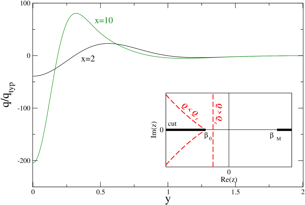
Figure 2: The quantity $q(k,t,t_{w})$ is plotted in $d=3$ against $y$ (for large $t_{w}$) and for two different choices of $x=t/t_{w}$. In the inset the analyticity region of h (Eq.(9)) and the steepest descent paths are plotted (dashed red).

Due to the sticking of $z_{steep}$, it consists of two parts. For ${\cal Q}\leq{\cal Q}_{c}$ it is linear. For ${\cal Q}>{\cal Q}_{c}$ it grows to a maximum and then falls off (again linearly for large ${\cal Q}$ since $z^{*}\to\beta_{M}$). The two branches merge at ${\cal Q}_{c}$ with a discontinuity in $d^{3}{\cal L}/d{\cal Q}^{3}$.

A singular behaviour qualitatively similar to that described above has been observed in the numerical simulations of the quenching dynamics of a disordered model for glassy systems crisrit . This may suggest a certain generality of the phenomenon in aging system and a possible common origin. Non-analytical large deviation functions have been also found in a stochastic dissipative model for a single particle farago , in simple non-equilibrium systems coupled with two reservoirs Visco ; schutz , and in diffusive models in the continuum limit jonasing ; kafri , always in stationary conditions. The singular behaviour in farago ; Visco ; schutz has been related to the occurring of rare and very large fluctuations in the initial distribution.

In the non-equilibrium setting considered here, the singular behavior of the distribution is related to the tying of the saddle point solution to the analyticity edge. This mechanism is mathematically similar to the one occurring in the equilibrium phase-transition. In that context, the zero wave vector fluctuations develop a macroscopic variance baxter ; condvs through a mechanism reminiscent of the Bose-Einstein condensation. A similar phenomenon is dynamically produced here in the realm of fluctuating quantities: when a large amount $V{\cal Q}<Q_{c}\equiv V{\cal Q}_{c}$ of heat is released, a macroscopic fraction $Q-Q_{c}$ is provided by the $k=0$ mode. This is a novel condensation mechanism for non-equilibrium fluctuations.

The large deviation function exhibits remarkable symmetry properties in the limit $t_{w}\to\infty$ with ${\cal Q}$ fixed. It can be shown that in this limit the first term (i.e. $-z{\cal Q}$) in Eq. (9) is dominant, implying that the above limit amounts to test the behavior of the tails of the heat probability distribution. In this regime one finds an expression where only $\tilde{\cal Q}={\cal Q}/q_{typ}$ and $x=t/t_{w}$ appear

$${\cal L}({\cal Q};t,t_{w})={\cal L}\,(\tilde{\cal Q};x),$$ (18)

with ${\cal L}(\tilde{\cal Q};x)=q_{typ}\beta_{0}\tilde{\cal Q}$ or ${\cal L}(\tilde{\cal Q};x)=q_{typ}\beta_{M}\tilde{\cal Q}$ for $\tilde{\cal Q}<0$ or $\tilde{\cal Q}>0$, respectively. This shows that in this process the same scaling symmetry, which holds for average quantities, underlies also the behavior of fluctuations. As a consequence, ${\cal L}({\cal Q};t,t_{w})$ takes the simple form of Eq. (18) when its arguments are measured in units of their reference value at the current age $t_{w}$ of the system. Moreover, using the expression of ${\cal L}(\tilde{\cal Q};x)$ one finds the asymmetry function

$${\cal L}({\cal Q};t,t_{w})-{\cal L}(-{\cal Q};t,t_{w})=-(\beta_{M}-\beta_{0}){\cal Q}.$$ (19)

Plugging this result into Eq. (14) one recovers a relation formally identical to Eq. (1). Notice however that the physical context is quite different: Eq. (1) holds for $t-t_{w}$ large, while the validity of Eq. (14) requires $V$ large. Apart from this difference, Eq. (19) shows that, by virtue of a scaling symmetry, a fluctuation relation like (1) may be obeyed also in systems that are not at stationarity, but are slowly relaxing and aging. To the best of our knowledge, this is the first analytical result showing this in a classical model of statistical mechanics with a non-trivial equilibrium phase diagram. The quantities $\beta_{0},\beta_{M}$ represent the origin of the cuts of $h$, and in close analogy to the equilibrium case can be regarded as self-generated internal temperatures. According to Eq. (19) these regulate large heat fluxes. Recalling that $-\beta_{0}=q^{-1}(k=0)$ and $\beta_{M}=q^{-1}(k=k_{M})$, such temperatures can be naturally associated to the ordering modes releasing energy at $\vec{k}=0$, and to those absorbing heat at a finite wave vector $\vec{k}_{M}=y_{M}t_{w}^{-1/2}$ (see Fig. 2). Notice that, for $t_{w}\to\infty$ and fixed $x$, $\beta_{0}$ and $\beta_{M}$ decrease to zero as $q_{typ}^{-1}=t_{w}^{1-d/2}$. Interestingly enough, this is the same behavior observed for the so called effective temperature $\beta_{eff}$, defined in terms of the ratio between the response and the correlation functions, in the present model noi2002 . However, the relation between the quantities $\beta_{0}$, $\beta_{M}$ entering $P(Q;t,t_{w})$ and $\beta_{eff}$ remains to be fully clarified.

Finally, we briefly discuss the modifications introduced to the present picture by a quench to a finite temperature. It has been shown noi2002 that, in this case, the order parameter can be split into two statistically independent fields $\boldsymbol{\varphi}=\boldsymbol{\sigma}+\boldsymbol{\psi}$, where $\boldsymbol{\sigma}$ and $\boldsymbol{\psi}$ are, respectively, an ordering and a thermal fluctuation component. In the scalar case ($N=1$), these two terms are associated to the slow aging process caused by the displacement of interfaces and to the fast spin fluctuations with equilibrium character inside the bulk of the domains. This additive property amounts to the splitting $C=C^{(\sigma)}+C^{(\psi)}$ of the correlation entering our calculations. In noi2002 it is shown that $C^{(\psi)}$ is the equilibrium correlation at the quench temperature $T$, while $C^{(\sigma)}$ behaves as in a quench to $T=0$, apart from some trivial non-universal constants. Then, in place of Eq.(8), one arrives at

$$P(Q;t,t_{w})=\int_{-i\infty+z_{0}}^{+i\infty+z_{0}}\frac{dz}{2\pi i}\,e^{V\left[h^{(\sigma)}+h^{(\psi)}+h^{(\sigma\psi)}\right]},$$ (20)

where $h^{(\sigma)}$ and $h^{(\psi)}$ are given by Eq. (9) by setting the correlator $C=C^{(\sigma)}$ or $C=C^{(\psi)}$ respectively, and $h^{(\sigma\psi)}$ is a function containing cross products $C^{(\sigma)}C^{(\psi)}$. In the limit $t_{w}\to\infty$ with fixed $x$, or alternatively with $t-t_{w}$ fixed, it is possible to show that the cross-term $h^{(\sigma\psi)}$ can be neglected. Hence the heat probability results as the convolution

$$P=P^{(\psi)}\,*\,P^{(\sigma)}=(2\pi i)^{-1}\int_{-i\infty+z_{0}}^{i\infty+z_{0}}dz\,e^{V\left[h^{(\psi)}+h^{(\sigma)}\right]}$$ (21)

of the fast and slow degree distributions. $P^{(\sigma)}$ has the properties discussed insofar for the quench to $T=0$ while $P^{(\psi)}$ is the equilibrium distribution at the temperature $T$. Notice that, in the regime $t_{w}\to\infty$ with $t-t_{w}$ fixed, $h^{(\sigma)}$ is negligible and one remains with the equilibrium distribution alone $P=P^{(\psi)}$. With these behaviors, it can be shown that the saddle point structure described above is not changed, except for a shift of the branch points at $\beta_{0},\beta_{M}$ Then a singularity in the large deviation function occurs at a temperature dependent ${\cal Q}_{c}(T)<0$. As it can be seen in Fig. 1, the convolution with the equilibrium part, produces a broadening of ${\cal L}$ particularly for large $T$ and/or small $x$. This convolution structure, shown here for the first time, is expected to be very general in aging systems where a wide separation of time scales occurs, and also appropriate for other fluctuating quantities, beside $Q$. We notice that an analogue property is not expected in critical quenches at $T=T_{c}$ where the additivity $\boldsymbol{\varphi}=\boldsymbol{\sigma}+\boldsymbol{\psi}$ is not obeyed: The composition of equilibrium and off-equilibrium fluctuations in this case remains an interesting issue to be clarified.

By summarizing, we have computed the exact asymptotic probability distribution of the heat exchanged by a quenched ferromagnet described by the large-$N$ model. A rich scaling structure emerges where heat, released by the small wave vector ordering modes, flows to components with finite wave vectors. The heat large deviation function shows a non-differentiable behavior with a singular threshold $Q_{c}$ signalling the onset of fluctuations condensation at zero wave vector. Heat currents are governed by a fluctuation relation analogue to the one obeyed in stationary systems in contact with two baths, but here with two self-generated temperatures $\beta_{0}$, $\beta_{M}$. It is a challenge to establish to what extent the scenario above outlined is generic and holds also for systems with finite $N$.

- (1) H. Touchette and R J. Harris, Large deviation approach to nonequilibrium systems, in R. Klages, W. Just, C. Jarzynski (eds), Nonequilibrium Statistical Physics of Small Systems: Fluctuation Relation and Beyond (Wiley-VCH, Weinheim, 2012).
- (2) L. Bertini et al, J. Stat. Phys. 107, 635 (2002); Phys. Rev. Lett. 87, 040601 (2001); J. Stat. Mech. P07014 (2007). T. Bodineau and B. Derrida, Phys. Rev. Lett. 92, 180601 (2004). J. Tailleur, J. Kurchan, and V. Lecomte, Phys. Rev. Lett. 99, 150602 (2007).
- (3) D.J. Evans et al., Phys. Rev. Lett. 71, 2401 (1993); G. Gallavotti, E.G.D. Cohen, J. Stat. Phys. 80, 931 (1995).
- (4) For a recent review see U. Seifert arXiv:1205.4176v1 [cond-mat.stat-mech].
- (5) C. Jarzynski and D.K. Wojcik, Phys. Rev. Lett. 92, 230602 (2004).
- (6) T. Bodineau and B. Derrida, C.R. Physique 8, 540 (2007).
- (7) A. Crisanti and F. Ritort, Europhys. Lett. 66, 253 (2004); F. Ritort, J. Phys. Chem. B 108, 6893 (2004).
- (8) A. Imparato et al, Phys Rev. E 76, 050101(R) (2007).
- (9) J.R. Gomez-Solano et al., Phys. Rev. Lett. 106, 200602 (2011).
- (10) L. F. Cugliandolo and J. Kurchan, Phys. Rev. Lett. 71, 173 (1993); J. Phys. A 27, 5749 (1994). L.F. Cugliandolo, J. Phys. A 44, 483001 (2011).
- (11) A.J. Bray, Adv. Phys. 43, 357 (1994).
- (12) T.H. Berlin, and M. Kac, Phys. Rev. 86, 821 (1952).
- (13) C. Castellano, F. Corberi, and M. Zannetti, Phys. Rev. E 56, 4973 (1997); N.Fusco and M.Zannetti, Phys. Rev. E 66, 066113 (2002).
- (14) A. Coniglio and M. Zannetti, Europhys. Lett. 10, 575 (1989).
- (15) F. Corberi, E. Lippiello, and M. Zannetti, Phys. Rev. E 65, 046136 (2002).
- (16) R.J. Baxter, Exactly Solved Models in Statistical Mechanics (Academic, London, 1982).
- (17) J. Farago, J. Stat. Phys. 107, 781 (2002); Physica A 331, 69 (2004).
- (18) P. Visco, J. Stat. Mech P06006 (2006).
- (19) R.J. Harris, A. Rákos, and G.M. Schütz, Europhys. Lett. 75 227 (2006).
- (20) G. Bunin, Y. Kafri, and D. Podolsky, arXiv:1207.6117 [cond-mat].
- (21) L. Bertini et al, J. Stat. Mech. L11001, (2010).