Ultraviolet Measurements of Interstellar C₂

Abstract

We analyzed archival spectra acquired with the Hubble Space Telescope for a study of interstellar C₂. Absorption from the electronic transitions, $D$ ${}^{1}\Sigma^{+}_{\rm u}$ – $X$ ${}^{1}\Sigma^{+}_{\rm g}$ (0,0) as well as $F$ ${}^{1}\Pi_{\rm u}$ – $X$ ${}^{1}\Sigma^{+}_{\rm g}$ (0,0) and (1,0), was the focus of the study. Our profile syntheses revealed that the lines of the $F-X$ bands were broadened as a result of a perturbation involving the upper levels. Further evidence for the perturbation came from anomalies in line strength and position for the $F-X$ (0,0) band. The perturbation likely arises from a combination of triplet-singlet interactions involving spin-orbit mixing between ${}^{3}\Pi_{\rm u}$ states and $F$ ${}^{1}\Pi_{\rm u}$ and an avoided crossing between the ${}^{3}\Pi_{\rm u}$ states. Tunneling through a potential barrier caused by the 3 and 4 ${}^{1}\Pi_{\rm u}$ states and spin-orbit mixing with other close-lying triplet states of $ungerade$ symmetry are less likely. Except for the broadening, lines in the $F-X$ (1,0) band appear free from anomalies and can be used to study interstellar C₂; new results for 10 sight lines are presented.

1 Introduction

The C₂ molecule is a useful diagnostic of the physical conditions in diffuse molecular clouds. Analysis of its rotational excitation provides information on kinetic temperature, density of collision partners [$n_{coll}$ $=$ $n$(H I) $+$ $n$(H₂)], and the flux of near infrared radiation permeating the gas (van Dishoeck & Black 1982). Because it acts as an intermediary in the chemical sequence leading to CN in these clouds (Federman et al. 1984; Federman et al. 1994), modeling this chemistry allows one to infer the total gas density [$n_{H}$ $=$ $n$(H I) $+$ 2 $n$(H₂)] and the ultraviolet (UV) flux incident on the cloud. Many studies have extracted this information from measurements of absorption from the series of bands in the $A-X$ Phillips system (e.g., Chaffee et al. 1980; Hobbs & Campbell 1982; Danks & Lambert 1983; van Dishoeck & de Zeeuw 1984; van Dishoeck & Black 1989; Federman et al. 1994; Sonnentrucker et al. 2007; Kaźmierczak et al. 2010).

The molecule also reveals absorption at near and far UV wavelengths, which is the focus of our work. Using the $Copernicus$ satellite, Snow (1978) reported a tentative detection of absorption from the R(0) line of the Mulliken $D-X$ (0,0) band near 2313 Å toward $\zeta$ Oph. Observations with the International Ultraviolet Explorer revealed absorption from the $F-X$ (0,0) band at 1342 Å (Lien 1984) toward X Per, but the $D-X$ (0,0) and $F-X$ (1,0) bands were not seen. Lien (1984) suggested that the oscillator strength ($f$-value) for the $F-X$ (0,0) band was at least 0.10. Lambert et al. (1995) detected absorption from the two (0,0) bands toward $\zeta$ Oph, using the Goddard High Resolution Spectrograph (GHRS) on the Hubble Space Telescope ($HST$). They inferred an $f$-value for the $F-X$ (0,0) band ($f_{00}^{F-X}$) of $0.10\pm 0.01$ based on a comparison of the amount of absorption relative to that seen from the $D-X$ (0,0) band. A theoretical value of 0.0545 for $f_{00}^{D-X}$ (Chabalowski et al. 1983; Bruna & Wright 1992) was adopted for the comparison. A surprising finding from their analysis was that Lambert et al. had problems fitting the band profile. The P(6) and Q(12) lines were too weak, the P(8) and Q(14) lines were absent, and the amount of absorption was too strong between 1342.5 and 1343.0 Å. We note that absorption from only even levels is observed.

Subsequent analysis of $HST$ observations revealed further information about the UV transitions in C₂. Kaczmarczyk (2000) examined absorption toward X Per from the $F-X$ (0,0) band and found additional line anomalies. Starting from the results from the $D-X$ band, Kacmarczyk showed that R($J^{\prime\prime}>2$), Q(8), Q(10), and P(4) were too weak. In a detailed study, Sonnentrucker et al. (2007) expanded upon this work. First, they obtained a better fit to line positions for the $D-X$ band by adopting $\nu_{0}$ $=$ 43227.2 cm^-1 from Sorkhabi et al. (1998). They also noted that a shift in line position occurred for lines involving $J^{\prime\prime}$ $<$ 10 for the $F-X$ (0,0) band. Sonnentrucker et al. pointed out that the anomalies seen in the $F-X$ (0,0) band did not arise from stellar features in the background continuum because the stars in their sample had different spectral types, $v$ sin$i$, etc. In the end, the fits to the $D-X$ (0,0) and $F-X$ (1,0) bands were very good, when $f_{10}^{F-X}$ of about 0.06 was used.

Through further analysis, we refine our knowledge of the perturbation(s) responsible for the line anomalies. As in Lambert et al. (1995) and Sonnentrucker et al. (2007), we start with syntheses of the $D-X$ band. Since we also find fits to the $F-X$ (1,0) band that are quite good, we extract C₂ column densities for directions where we obtained CO abundances from the far UV spectra previously (Pan et al. 2005; Sheffer et al. 2008). The data for our study are described in § 2, as is our method of processing the spectra, and § 3 provides the results of our analyses. They are discussed in § 4. We summarize our findings in the final Section.

2 Data and Their Analysis

The spectra were downloaded from the $HST$ archive at the Multiwavelength Archive at the Space Telescope Science Institute (MAST) as part of our earlier studies. In particular, we used the GHRS spectra described by Lambert et al. (1995), but analyzed it together with spectra from the Space Telescope Imaging Spectrograph (STIS) in a self-consistent manner. Far UV spectra acquired with STIS for our CO studies (Pan et al. 2005; Sheffer et al. 2008) comprised the bulk of the sample. As for the near UV spectra obtained with STIS that contain absorption from the $D-X$ band, we downloaded the same exposures as Sonnentrucker et al. (2007), but analyzed them in an independent manner. Our analyses are based on rectified spectra, where the stellar continuum was removed through fits involving low-order polynomials in most cases. In some cases, such as for the $F-X$ bands seen in the spectrum of HD 203532, stellar features had to be fitted and removed as well.

The initial focus was on the directions with absorption from all three bands – HD 24534 (X Per), HD 27778 (62 Tau), HD 147888 ($\rho$ Oph D), HD 149757 ($\zeta$ Oph), and HD 207198. The spectra of $\zeta$ Oph were from GHRS observations. Because the spectra for X Per revealed strong absorption and had high signal to noise, they were analyzed first; analysis of the spectra for the four other sight lines provided confirmation of our results regarding the perturbations involving the $F-X$ transitions. In light of the ability of Lambert et al. (1995) and Sonnentrucker et al. (2007) to fit the $D-X$ band with confidence, we synthesized this band first, basing it on resolving powers of 80,000 for the GHRS spectrum and about 100,000 for STIS and on an $f$-value of 0.0545. The component structures used in the syntheses come from our earlier work (Lambert et al. 1995; Sheffer et al. 2008). Pan et al. (2005) described the close correspondence in component structure for CO and CN, providing evidence that these two molecules coexist in the core of diffuse molecular clouds. Chemical studies (e.g., Federman et al. 1994) and analyses of CO and C₂ excitation (Sheffer et al. 2007) indicate that the C₂ molecule is also in the core. For comparison, Sonnentrucker et al. (2007) synthesized the C₂ transitions through a combination of the component structure seen in K I, CH, and CN absorption.

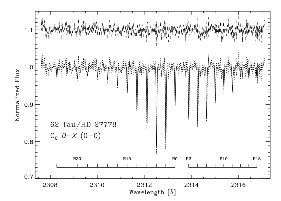
Figure 1: Absorption from the $D-X$ band of C₂ toward HD 27778. The dotted line indicates data normalized to unity, while the solid line is the fit based on component structure used by Sheffer et al. (2008) for CO. Individual transitions are identified at the bottom of the figure. The residuals appear above the spectrum at 1.1 as a dashed line.

We adopted the line lists given by Sonnentrucker et al. (2007) for our profile syntheses with the code ISMOD (see §2.5 in Sheffer et al. 2008). We also found that improved fits to the $D-X$ band arise when the constants from Sorkhabi et al. (1998) are adopted. The fits to the $D-X$ band yielded column densities for individual rotational levels of the molecule. These column densities then were applied to the $F-X$ bands, where we allowed the band $f$-value and line width to vary. By allowing the line width to vary, we were able to search for intrinsic broadening associated with the perturbations seen in earlier studies. An example of our fits to the $D-X$ and $F-X$ bands toward 62 Tau (HD 27778) is shown in Figures 1 and 2, respectively. Once a self-consistent set of $f$-values and intrinsic line broadening for the $F-X$ bands were found, we were able to extract C₂ column densities for additional sight lines. Examples appear in Fig. 3.

3 Results

3.1 $F-X$ Bands

We confirm earlier astronomical analyses of these bands. We find that the $f$-values for the (0,0) band (0.10, Lambert et al. 1995) and (1,0) band (0.06, Sonnentrucker et al. 2007) provide a set of self-consistent oscillator strengths when used in combination with the $D-X$ (0,0) and $A-X$ (2,0) bands. We also observe the line anomalies noted by Lambert et al. (1995), Kacmarczyk (2000), and Sonnentrucker et al. (2007).

We go beyond this body of work in two important ways, based mainly on absorption toward X Per whose spectra have the highest signal to noise. First, we are best able to fit the lines in the two $F-X$ bands with a resolving power of 60,000, significantly lower that the resolving power achievable with STIS. We believe this results from increased intrinsic broadening arising from shortened lifetimes in levels of the $F$ state. A lifetime of about $6\times 10^{-12}$ s^-1, compared to typical radiative lifetimes of ns (see below), is inferred. Second, while Sonnentrucker et al. (2007) found that the $J^{\prime\prime}$ $<$ 10 lines of the $F-X$ (0,0) band are shifted by about 36 mÅ (or 8 km s^-1), we further quantify details about the shifts. We focus on the upper rotational levels where the perturbation is taking place. We find the following offsets in velocity (km s^-1) as a function of $J^{\prime}$.

$J^{\prime}$	1	2	3	4	5	6	7	8	9	10	11	12	13	14	15	16	17	18
offset	$+8.0$	$+8.0$	$+8.0$	$+8.0$	$+8.5$	$+9.0$	$+9.5$	$+8.0$	$+11.5$	$+15.0$	$+15.0$	$-2.0$	$0.0$	$+2.0$	$\ldots$	$0.0$	$\ldots$	$0.0$
(km s-1)

All levels with $J^{\prime}$ $\leq$ 11 show substantial shifts, with $J^{\prime}$ of 10 and 11 shifted by 5 resolution elements. No shift is seen for J^′ $\geq$ 12.

3.2 Interstellar C₂

The results of our syntheses appear in Tables 1 and 2. Table 1 gives column densities for individual rotational levels for the directions with $D-X$ spectra and comparisons to earlier analyses (Lambert et al. 1995; Kaczmarczyk 2000; Sonnentrucker et al. 2007), while Table 2 provides column densities for new sight lines. As expected, essentially all our results in Table 1 agree with the earlier determinations at the 1-$\sigma$ level. The largest differences appear for the $J$ $=$ 2 and 4 levels toward X Per, where our values are about 2-$\sigma$ larger. We also report tentative detections for $J$ $=$ 16 and 18 toward X Per and $\rho$ Oph D.

4 Discussion

4.1 $D-X$ Band

Before discussing the perturbations in the $F-X$ bands, we summarize the situation for the Mulliken band. The first studies of the radiative properties of C₂ molecules in the $D-X$ (0,0) band yielded laboratory lifetimes for the upper level. Using the phase shift method, Smith (1969) measured a lifetime of $14.6\pm 1.5$ ns for an $f$-value of $0.055\pm 0.06$. Curtis et al. (1976) obtained a lifetime of $18.1\pm 1.0$ ns on an unresolved group of lines with the High Frequency Deflection Technique. Subsequent studies relied on large-scale theoretical calculations. Chabalowski et al. (1983) performed a multireference double excitation – configuration interaction (MRD-CI) calculation that yielded a lifetime of 14 ns and an $f$-value of 0.054. The computation by Bruna & Wright (1992), also based on MRD-CI, gave a lifetime of 14.6 ns and $f$-value of 0.0546. Kokkin et al. (2007) used multireference configuration interaction (MRCI) techniques and found a ratio of oscillator strengths, $f_{20}^{A-X}$/$f_{00}^{D-X}$, of 0.0212 versus the ratio quoted by Lambert et al. (1995) of $0.0226\pm 0.029$, which was based on $f_{00}^{D-X}$ $=$ 0.0545. Most recently, Schmidt & Bacskery (2007) enlarged the scope of calculations performed by Kokkin et al. (2007) by incorporating non-orthogonal orbitals. Schmidt & Bacskery obtained a lifetime of 13.4 ns, an $f$-value of 0.0535, and a ratio of 0.0266. The value for $f_{00}^{D-X}$ seems quite secure.

4.2 $F-X$ Bands

The only laboratory-based spectroscopic study is that of Herzberg et al. (1969), whose molecular constants are used for analysis of interstellar absorption. The derivation of these constants relied on lines with $J^{\prime\prime}$ $\geq$ 10 for the most part. For the (0,0) band, laboratory data do not exist for lower values of $J^{\prime\prime}$, while data only on the Q branch of the (1,0) band are presented by Herzberg et al. (1969) for these rotational levels. Therefore, the only quantitative information for the perturbations involving the $F-X$ levels at the present time is based on astronomical spectra – broadened lines and line shifts of 8 to 15 km s^-1.

Several quantum mechanical calculations examined Rydberg states, such as $F$ ${}^{1}\Pi_{\rm u}$. The first one (Barsuhn 1972), which was based on self-consistent field and configuration interaction (SCF$+$CI), investigated the energies for the Rydberg states. Another SCF$+$CI calculation by Pouilly et al. (1983) focused on the C₂ photodissociation rate for chemical models of interstellar clouds and comets. They also determined a value for $f_{00}^{F-X}$of 0.02, which differs from $0.10\pm 0.01$ derived by Lambert et al. (1995) from interstellar spectra. The most comprehensive theoretical study to date (Bruna & Grein 2001) involved MRCI calculations of valence and Rydberg states between 7 and 10 eV. Bruna & Grein obtained $f_{00}^{F-X}$ of 0.098, in much better agreement with astronomical determinations. We are not aware of any reported calculation giving a value for $f_{10}^{F-X}$.

Our results suggest that the $v$ $=$ 0 level of the $F$ ${}^{1}\Pi_{\rm u}$ state is affected more than the $v$ $=$ 1 level because both line anomalies (in strength and position) and broadening are seen only in lines involving $v$ $=$ 0. We examine the theoretical results of Bruna & Grein (2001) in order to interpret the interstellar observations. They provide the following description of the $F$ (2 ${}^{1}\Pi_{\rm u}$) state. Its potential energy curve is affected by avoided crossings at about 2.8 Bohr with the curves associated with 3 ${}^{1}\Pi_{\rm u}$ and 4 ${}^{1}\Pi_{\rm u}$, yielding 3 bound vibrational levels for the $F$ state. We note that Herzberg et al. (1969) observed the lower two levels, which are also the only ones associated with interstellar spectra. The depth of the potential well is about 0.5 eV. The $F$ state not only is metastable regarding radiative emission, but it is also metastable with respect to predissociation. The latter arises because the minimum in the potential curve for the $F$ state lies about 1.50 eV above its diabatic limit, C[¹D] $+$ C[¹D]. The $F$ state is somewhat unique since the same potential curve undergoes two very different predissociation mechanisms before and after the minimum.

The likely cause for the perturbations seen by Lambert et al. (1995), Kaczmarczyk (2000), Sonnentrucker et al. (2007), and us involves triplet-singlet interactions, via spin-orbit mixing, and an avoided crossing. According to Bruna & Grein (2001), the curves for 2 and 3 ${}^{3}\Pi_{\rm u}$ are essentially repulsive. The inner portion of the 3 ${}^{3}\Pi_{\rm u}$ curve constitutes the triplet counterpart of $F$ ${}^{1}\Pi_{\rm u}$. There exists an avoided crossing between the curves for 2 and 3 ${}^{3}\Pi_{\rm u}$ at approximately 9.2 eV near 2.4 Bohr that may affect the $F$ ${}^{1}\Pi_{\rm u}$ potential. Beyond the avoided crossing, the curve for 3 ${}^{3}\Pi_{\rm u}$ lies close to that for $F$ ${}^{1}\Pi_{\rm u}$ for a short interval.

Portions of the potential curves for 4 and 5 ${}^{3}\Pi_{\rm u}$ are also located nearby (around 9.5 eV and internuclear separation of about 2.6 Bohr). Both curves have potential wells; Bruna & Grein (2001), however, do not list possible vibrational levels for 4 and 5 ${}^{3}\Pi_{\rm u}$. If they existed, triplet-singlet mixing may arise, but the line broadening seen by us suggests predissociation is taking place and that would require another avoided crossing with a repulsive curve.

Tunneling through the potential barrier created by avoided crossings among ${}^{1}\Pi_{\rm u}$ states and spin-orbit mixing between $F$ ${}^{1}\Pi_{\rm u}$ and other close-lying triplet states of $ungerade$ symmetry could also lead to the perturbations seen in interstellar spectra (P. Bruna, private communication), but are less likely. Tunneling is expected to affect the $v$ $=$ 2 level the most because it lies near the top of the barrier; such an effect may explain why lines from this level are not seen in laboratory (Herzberg et al. 1969) or interstellar spectra. The spin-orbit mixing considered here involves repulsive states that can predissociate the $F$ state. We consider the results of CI calculations by Kirby & Liu (1979). Their Table VI lists weakly bound states that may be of relevance here. Two states, 2 ${}^{3}\Sigma^{+}_{\rm u}$ and 1 ${}^{3}\Sigma^{-}_{\rm u}$, may perturb the $F$ state in a significant way. However, in a theoretical analysis of the interaction between the $X$ ${}^{1}\Sigma^{+}_{\rm g}$ and $b$ ${}^{3}\Sigma^{-}_{\rm g}$ states, Langhoff et al. (1977) pointed out that such interactions are relatively weak, since two electrons are excited.

4.3 Interstellar C₂

Since the results on C₂ based on the $D-X$ band toward the stars X Per, 62 Tau, $\rho$ Oph D, $\zeta$ Oph, and HD 207198 have been analyzed by us (e.g., Federman et al. 1994; Lambert et al. 1995; Sheffer et al. 2008) and others in the past (e.g., van Dishoeck & Black 1986; Kaczmarczyk 2000; Sonnentrucker et al. 2007), here we focus on the new determinations. We consider predictions for the C₂ column density inferred from observed columns of CH and CN, based on a simple prescription discussed by us earlier (e.g., Federman et al. 1994; Knauth et al. 2001). In particular, we compare the predictions in Pan et al. (2005) and Sheffer et al. (2008) with the C₂ measurements from the present work. Furthermore, the rotational state distribution in terms of column densities yields information about the excitation of the molecule, from which gas density and temperature and the strength of the infrared radiation field permeating the gas can be inferred (van Dishoeck & Black 1982).

More recent data indicate refinements to the analysis of C₂ excitation compared to our earlier studies. First, experiments (Erman & Iwamae 1995) and theoretical calculations (Kokkin et al. 2007; Schmidt & Bacskay 2007) are converging on a $f$-value for the $A-X$ (2,0) transition larger than we used in the past. A value of $1.4\times 10^{-3}$ now seems more appropriate, rather than $1.0\times 10^{-3}$ used by us in the past. Second, the cross section for excitation via collisions is larger than the value suggested by van Dischoek & Black (1982). More recent quantum mechanical calculations (Lavendy et al. 1991; Robbe et al. 1992; Najar et al. 2008, 2009) indicate a cross section of $4\times 10^{-16}$ cm², rather than $2\times 10^{-16}$ cm².

The two changes would partially cancel, yielding $n_{coll}$ about 60% smaller than what we would have obtained with the older values. However, a more sophisticated treatment based on the latest information and considering core-halo clouds (Casu & Cecchi-Pestellini 2012) suggests that our original method provides a reasonable approximation. This arises when a weighted density is obtained for the core and halo portions of the clouds seen toward $\zeta$ Oph, which we also studied (Lambert et al. 1995). We, therefore, present results using our earlier method with the realization of their approximate nature. To extract $n_{H}$ from $n_{coll}$, we continue to assume there is no enhancement in the infrared flux over the average interstellar value and we multiply $n_{coll}$ by 1.5. This accounts for the fact that diffuse molecular clouds have roughly equal amounts of atomic and molecular hydrogen.

Table 3 provides comparisons of measured and predicted C₂ column density, predicted gas densities from CN chemistry and C₂ excitation, and the gas temperature derived from H₂, $T_{01}$(H₂), and the C₂ excitation temperature, $T$(C₂), the latter based on all observed column densities. Our column densities appearing in the second column are obtained from the detections shown in Table 2; if contributions from higher-lying levels were included, $N$(C₂) would be about 0.1 dex higher. In the column for gas densities from analysis of the CN chemistry, several entries may appear, depending on the number of molecular components detected for that sight line. The C₂ column densities predicted by the simple CN chemical model agree very well with our new determinations. For HD 206267, HD 207308, and HD 208266, the comparison is best when only the main molecular component is considered. This is not surprising; although the complete component structure is used to fit the spectra, the other components are masked in the noise because the $F-X$ (1,0) band is relatively weak. For HD 206267, we also note that the column density inferred from the $F-X$ (0,0), $A-X$ (2,0), and $A-X$ (3,0) bands by Sonnentrucker et al. (2007) is in excellent agreement with our result. The gas densities derived from the CN chemistry and C₂ excitation do not appear to agree very well. The expected agreement is a factor of 2 (e.g., Federman et al. 1994), but the densities from excitation are generally lower. A possible cause for the discrepancy may involve the presence of multiple, lower density molecular components along the line of sight. Modeling the spectra may favor the dominant component in terms of column density, but the distribution of rotational levels may depend on all the components. Further evidence for this possibility is found in the comparison between $T_{01}$(H₂) and $T$(C₂). Except for the gas toward HD 192035, which has the highest density from C₂ excitation in our sample, the two temperatures are comparable. Earlier studies of molecular rich diffuse clouds (see e.g., Sheffer et al. 2007) showed that on average $T$(C₂) was less than $T_{01}$(H₂). The lower density, higher temperature components appear to play a more significant role in the determination of C₂ excitation. This idea is supported by the more thorough analyses of Casu & Cecchi-Pestellini (2012). We also mention that the excitation analysis for the gas toward HD 198781 is not very satisfying. Minimizing the differences between the observable distribution and the predicted ones could not provide restrictions on $T$(C₂). This probably arose because absorption from only $J^{\prime\prime}$ $=$ 4 and 6 was detected.

5 Conclusions

We described a study of interstellar C₂ based on archival $HST$ spectra of the $D-X$ (0,0), $F-X$ (0,0), and $F-X$ (1,0) bands. Building on earlier work, we provided further details regarding the anomalies in line strengths seen in the $F-X$ (0,0) band. Line shifts were quantified for transitions involving $J^{\prime}$ $\leq 11$. The lines for both $F-X$ bands were found to be broadened by predissociation. The anomalies likely arise from triplet-singlet interactions involving spin-orbit mixing between the $F$ ${}^{1}\Pi_{u}$ state and ${}^{3}\Pi_{\rm u}$ states combined with an avoided crossing between the triplet states. Other possibilities include tunneling through a potential barrier, which is caused by avoided crossings with the 3 and 4 ${}^{1}\Pi_{u}$ states, and spin-orbit mixing between the $F$ state and other triplet states of $ungerade$ symmetry, but these are not as likely. We also determined new C₂ column densities from the $F-X$ (1,0) band and compared these results with our earlier predictions, finding very good agreement. Our analysis of C₂ excitation yields somewhat lower gas densities, but these are consistent with core-halo models using a refined set of input parameters (Casu & Cecchi-Pestellini 2012). The inferred gas densities are still consistent with chemical predictions, when the presence of complex component structure along the line of sight having a range of gas densities is considered.

We conclude by noting possible extensions of this work. First, additional theoretical calculations and experiments are needed to elucidate more clearly the cause of the anomalies present in $F-X$ spectra. Second, because empirical and theoretical oscillator strengths for the three band systems used in interstellar studies ($A-X$, $D-X$, $F-X$) have achieved an impressive level of concensus, interstellar C₂ abundances are now more secure. Abundances can be determined from any of the bands, but analyses should not rely solely on the $F-X$ (0,0) band, where anomalies in line strength are the strongest. Future studies using the $F-X$ bands should also incorporate the broadening caused by predissociation when modeling the spectra. This is especially important for studies of sight lines where the transition from diffuse molecular to dark clouds is taking place. The abundances are sufficiently large that optical depth effects need to be considered.

Table 1: Column Densities for C₂ $D-X$ (0,0)

Level	X Per				62 Tau			$\rho$ Oph D			$\zeta$ Oph			HD 207198
	Present	K00	SWTY07		Present	SWTY07		Present	SWTY07		Present	LSF95		Present	SWTY07
$J$ = 0	0.165(0.024),	0.153(0.051)	0.15(0.02)		0.166(0.012)	0.15(0.02)		0.099(0.010)	0.10(0.02)		0.069(0.005)	0.075(0.015)		0.218(0.028)	0.20(0.02)
$J$ = 2	0.774(0.051)	0.648(0.075)	0.67(0.05)		0.594(0.026)	0.57(0.04)		0.319(0.021)	0.33(0.02)		0.302(0.012)	0.290(0.024)		0.883(0.175)	0.83(0.04)
$J$ = 4	0.784(0.049)	0.674(0.083)	0.69(0.04)		0.633(0.024)	0.62(0.04)		0.367(0.022)	0.37(0.03)		0.356(0.011)	0.327(0.019)		0.984(0.102)	0.91(0.05)
$J$ = 6	0.592(0.049)	0.530(0.069)	0.55(0.04)		0.480(0.023)	0.47(0.03)		0.277(0.020)	0.28(0.02)		0.266(0.008)	0.247(0.019)		0.822(0.083)	0.75(0.04)
$J$ = 8	0.395(0.046)	0.346(0.062)	0.37(0.04)		0.331(0.024)	0.32(0.03)		0.151(0.023)	0.18(0.02)		0.200(0.010)	0.192(0.020)		0.537(0.072)	0.51(0.04)
$J$ = 10	0.293(0.037)	0.291(0.063)	0.23(0.03)		0.189(0.020)	0.19(0.02)		0.128(0.025)	0.14(0.02)		0.145(0.010)	0.137(0.017)		0.335(0.032)	0.37(0.04)
$J$ = 12	0.184(0.035)	0.177(0.056)	0.22(0.03)		0.171(0.021)	0.15(0.02)		0.081(0.015)	0.08(0.02)		0.097(0.010)	0.111(0.014)		0.226(0.053)	0.23(0.04)
$J$ = 14	0.132(0.037)	0.139(0.045)	0.16(0.03)		0.106(0.017)	0.11(0.02)		0.037(0.015)	0.05(0.02)		0.084(0.009)	0.077(0.015)		0.165(0.057)	0.17(0.04)
$J$ = 16	0.094(0.030)	$\ldots$	0.04(0.03)		0.092(0.019)	0.09(0.02)		0.052(0.020)	$\ldots$		0.064(0.008)	0.062(0.016)		0.116(0.024)	0.13(0.04)
$J$ = 18	0.060(0.025)	$\ldots$	$\ldots$		0.067(0.020)	0.06(0.02)		0.060(0.020)	$\ldots$		0.049(0.008)	0.060(0.014)		0.109(0.029)	0.13(0.04)

Table 2: Equivalent Widths and Column Densities for C₂ $F-X$ (1,0)

Level	Branch	$W_{\lambda}$	$N_{J}$	$W_{\lambda}$	$N_{J}$	$W_{\lambda}$	$N_{J}$	$W_{\lambda}$	$N_{J}$	$W_{\lambda}$	$N_{J}$
		HD 23478		HD 147683		HD 177989		HD 192035		HD 198781
		$\pm$0.33		$\pm$0.38		$\pm$0.35		$\pm$0.60		$\pm$0.66
$J$ = 0	$R$	1.19	12.13$\pm$0.11	0.76	11.94$\pm$0.18	1.78	12.35$\pm$0.08	3.00	12.58$\pm$0.08	$\cdots$	$<$12.16
$J$ = 2	$R$	1.58	12.66$\pm$0.07	1.18	12.55$\pm$0.10	1.78	12.59$\pm$0.09	3.57	13.06$\pm$0.06	$\cdots$	$<$12.42
	$Q$	1.96		1.44		1.28		4.28		$\cdots$
	$P$	$\cdots$		$\cdots$		1.56		$\cdots$		$\cdots$
$J$ = 4	$R$	1.27	12.64$\pm$0.07	1.61	12.78$\pm$0.07	0.95	12.53$\pm$0.10	2.13	12.89$\pm$0.08	1.47	12.76$\pm$0.12
	$Q$	1.87		2.27		1.37		3.05		2.03
	$P$	$\cdots$		0.86		$\cdots$		$\cdots$		$\cdots$
$J$ = 6	$R$	0.67	12.39$\pm$0.12	1.03	12.60$\pm$0.09	$\cdots$	$<$12.20	$\cdots$	12.56$\pm$0.14	1.35	12.75$\pm$0.12
	$Q$	1.08		1.59		$\cdots$		1.56		2.00
	$P$	$\cdots$		$\cdots$		$\cdots$		$\cdots$		$\cdots$
$J$ = 8	$R$	0.74	12.45$\pm$0.10	1.21	12.69$\pm$0.08	$\cdots$	12.21$\pm$0.18	$\cdots$		$\cdots$
	$Q$	1.25		1.93		0.70		$\cdots$		$\cdots$
	$P$	$\cdots$		$\cdots$		$\cdots$		$\cdots$		$\cdots$
$J$ = 10	$R$	$\cdots$		$\cdots$		$\cdots$	12.23$\pm$0.17	$\cdots$		$\cdots$
	$Q$	$\cdots$		$\cdots$		0.73		$\cdots$		$\cdots$
	$P$	$\cdots$		$\cdots$		$\cdots$		$\cdots$		$\cdots$
		HD 203532		HD 206267		HD 207308		HD 208266		HD 220057
		$\pm 0.55$		$\pm 0.53$		$\pm 0.53$		$\pm 0.42$		$\pm 0.72$
$J$ = 0	$R$	1.78	12.35$\pm$0.12	3.50	12.70$\pm$0.06	2.79	12.54$\pm$0.08	2.89	12.57$\pm$0.06	$\cdots$	$<$12.14
$J$ = 2	$R$	2.81	12.99$\pm$0.07	4.32	13.23$\pm$0.04	3.55	13.06$\pm$0.05	2.07	12.81$\pm$0.07	$\cdots$	$<$12.54
	$Q$	3.31		5.03		4.26		2.52		$\cdots$
	$P$	$\cdots$		1.39		$\cdots$		$\cdots$		$\cdots$
$J$ = 4	$R$	2.24	12.95$\pm$0.07	3.76	13.23$\pm$0.04	3.73	13.17$\pm$0.04	1.97	12.86$\pm$0.06	$\cdots$	12.50$\pm$0.18
	$Q$	3.08		4.99		5.14		2.80		1.38
	$P$	1.24		2.16		2.05		1.05		$\cdots$
$J$ = 6	$R$	1.50	12.78$\pm$0.09	1.48	12.77$\pm$0.09	2.08	12.91$\pm$0.07	1.36	12.72$\pm$0.08	$\cdots$	12.61$\pm$0.15
	$Q$	2.26		2.26		3.19		2.11		1.73
	$P$	$\cdots$		$\cdots$		1.35		0.88		$\cdots$
$J$ = 8	$R$	$\cdots$	12.59$\pm$0.13	$\cdots$	12.57$\pm$0.13	1.27	12.70$\pm$0.10	$\cdots$	$<$12.27	$\cdots$	12.66$\pm$0.14
	$Q$	1.58		1.51		2.07		$\cdots$		1.92
	$P$	$\cdots$		$\cdots$		$\cdots$		$\cdots$		$\cdots$
$J$ = 10	$R$	$\cdots$	12.65$\pm$0.12	$\cdots$		1.15	12.67$\pm$0.10	$\cdots$	12.42$\pm$0.14	$\cdots$	$<$12.43
	$Q$	1.75		$\cdots$		1.94		1.13		$\cdots$
	$P$	$\cdots$		$\cdots$		$\cdots$		$\cdots$		$\cdots$
$J$ = 12	$R$	$\cdots$	12.47$\pm$0.16	$\cdots$		$\cdots$	12.61$\pm$0.12	$\cdots$		$\cdots$	$<$12.44
	$Q$	1.22		$\cdots$		1.72		$\cdots$		$\cdots$
	$P$	$\cdots$		$\cdots$		$\cdots$		$\cdots$		$\cdots$

Table 3: Comparison of Results

Star	log $N$(C2)	log $N_{p}$(C2)	$n_{H}$(CN)	$n_{H}$(C2)	$T_{01}$(H2)	$T$(C2)
			(cm-3)	(cm-3)	(K)	(K)
HD 23478	13.19(0.09)	13.18	325, 775	190	55	20–40
HD 147683	13.29(0.11)	$\ldots$	$\ldots$	95	58	50–60
HD 177989	13.11(0.13)	$\ldots$	$\ldots$	210	49	20
HD 192035	13.43(0.10)	13.52	$\leq$575, 1550 $\leq$725	350	68	20–30
HD 198781	13.06(0.16)	13.12	750	$\leq$95	65	10–100
HD 203532	13.58(0.09)	$\ldots$	$\ldots$	210	47	20–40
HD 206267	13.69(0.06)	13.81	80, 1150, 525, 60	280	65	20–40
	13.68(0.04)	13.70
HD 207308	13.71(0.07)	13.90	600, 300	190	57	20–50
	$\ldots$	13.79
HD 208266	13.40(0.09)	13.66	375, 90, 125	210	$\ldots$	10
	$\ldots$	13.52
HD 220057	13.07(0.22)	13.07	750, $\leq$850	165	65	90

Figure 2: As Fig. 1 for absorption from the $F-X$ bands of C₂ toward HD 27778. The upper panel shows the fit to the (0,0) band and the lower panel that for the (1,0) band. The fits were based on the column density derived from the $D-X$ band as presented in Fig. 1.

Figure 3: As Fig. 1 for absorption from the $F-X$ (1,0) band of C₂ toward HD 220057, HD 192035, and HD 203532, a sample of stars revealing new detections of C₂. The three stars are arranged from top to bottom according to $N$(C₂). Models show absorption from $J$ levels that are securely determined as presented in Table 2. Spectra of HD 220057 and HD 192035 have been shifted by $-0.120$ and $-0.128$ Å, respectively, to match the wavelength scale of HD 203532. HD 192035 was observed with the lower-resolution grating E140M.

References

- Barsuhn (1972) Barsuhn, J. 1972, Z. Naturforsch., A27, 1031
- Bruna & Grein (2001) Bruna, P. J., & Grein, F. 2001, Canadian J. Phys., 79, 653
- Bruna & Wright (1992) Bruna, P. J., & Wright, J. S. 1992, J. Phys. Chem., 96, 1630
- Casu & Cecchi-Pestellini (2012) Casu, S., & Cecchi-Pestellini, C. 2012, ApJ, 749, 48
- Chabalowski et al. (1983) Chabalowski, C. F., Peyerimhoff, S. D., & Buenker, R. J. 1983, Chem. Phys. 81, 57
- Chaffee et al. (1980) Chaffee, F. C., Lutz, B. L., Black, J. H., vanden Bout, P. A., & Snell, R. A. 1980, ApJ, 236, 474
- Curtis et al. (1976) Curtis, L., Engman, B., & Erman, P. 1976, Phys. Scripta, 13, 270
- Danks & Lambert (1983) Danks, A. C., & Lambert, D. L. 1983, A&A, 124, 188
- Erman & Iwamae (19995) Erman, P., & Iwamae, A. 1995, ApJ, 450, L31
- Federman et al. (1984) Federman, S. R., Danks, A. C., & Lambert, D. L. 1984, ApJ, 287, 219
- Federman et al. (1994) Federman, S. R., Strom, C. J., Lambert, D. L., et al. 1994, ApJ, 424, 772
- Herzberg et al. (1969) Herzberg, G., Lagerqvist, A., & Malmberg, C. 1969, Canadian J. Phys., 47, 2735
- Hobbs & Campbell (1982) Hobbs, L. M., & Campbell, B. 1982, ApJ, 254, 108
- Kaczmarczyk (2000) Kaczmarczyk, G. 2000, Acta Astron., 50, 151
- Kaźmierczak et al. (2010) Kaźmierczak, M., Schmidt, M. R., Bondar, A., & Krelowski, J. 2010, MNRAS, 402, 2548
- Kirby & Liu (1979) Kirby, K., & Liu, B. 1979, J. Chem. Phys., 70, 893
- Knauth et al. (2001) Knauth, D. C., Federman, S. R., Pan, K., Yan, M., & Lambert, D. L. 2001, ApJS, 135, 201
- Kokkin et al. (2007) Kokkin, D. L., Bacskay, G. B., & Schmidt, T. W. 2007, J. Chem. Phys., 126, 084302
- Lambert et al. (1995) Lambert, D. L., Sheffer, Y., & Federman, S. R. 1995, ApJ, 438, 740
- Langhoff et al. (1977) Langhoff, S. R., Sink, M. L., Pritchard, R. H., et al. 1977, J. Chem. Phys., 67, 1051
- Lavendy et al. (1991) Lavendy, H., Robbe, J. M., Chambaud, G., Levy, B., & Roueff, E. 1991, A&A, 251, 365
- Lien (1984) Lien, D. J. 1984, ApJ, 287, L95
- Najar et al. (2008) Najar, F., Ben Abdallah, D., Jaidane, N., & Ben Lakhdar, Z. 2008, Chem. Phys. Lett., 460, 31
- Najar et al. (2009) Najar, F., Ben Abdallah, D., Jaidane, N., et al. 2009, J. Chem. Phys., 130, 204305
- Pan et al. (2005) Pan, K., Federman, S. R., Sheffer, Y., & Andersson, B.-G. 2005, ApJ, 633, 986
- Pouilly et al. (1983) Pouilly, B., Robbe, J. M., Schamps, J., & Roueff, E. 1983, J. Phys. B, 16, 437
- Robbe et al. (1992) Robbe, J. M., Lavendy, H., Lemoine, D., & Pouilly, B. 1992, A&A, 256, 679
- Schmidt & Bacskery (2007) Schmidt, T. W., & Bacskay, G. B. 2007, J. Chem. Phys., 127, 234310
- Sheffer et al. (2008) Sheffer, Y., Rogers, M., Federman, S. R., et al. 2008, ApJ, 687, 1075
- Sheffer et al. (2007) Sheffer, Y., Rogers, M., Federman, S. R., Lambert, D. L., & Gredel, R. 2007, ApJ, 667, 1002
- Smith (1969) Smith, W. H. 1969, ApJ, 156, 791
- Snow (1978) Snow, T. P. 1978, ApJ, 220, L93
- Sonnentrucker et al. (2007) Sonnentrucker, P., Welty, D. E., Thorburn, J. A., & York, D. G. 2007, ApJS, 168, 58
- Sorkhabi et al. (1998) Sorkhabi, O., Xu, D. D., Blunt, V. M., et al. 1998, J. Mol. Spectrosc., 188, 200
- van Dishoeck & Black (1982) van Dishoeck, E. F., & Black, J. H. 1982, ApJ, 258, 533
- van Dishoeck & Black (1986) , 1986, ApJS, 62, 109
- van Dishoeck & Black (1989) , 1989, ApJ, 340, 273
- van Dishoeck & de Zeeuw (1984) van Dishoeck, E. F., & de Zeeuw, T. 1984, MNRAS, 206, 383