ASGARD: A Large Survey for Slow Galactic Radio Transients.
I. Overview and First Results

Abstract

Searches for slow radio transients and variables have generally focused on extragalactic populations, and the basic parameters of Galactic populations remain poorly characterized. We present a large 3 GHz survey performed with the Allen Telescope Array (ATA) that aims to improve this situation: ASGARD, the ATA Survey of Galactic Radio Dynamism. ASGARD observations spanned 2 years with weekly visits to 23 deg² in two fields in the Galactic Plane, totaling 900 hr of integration time on science fields and making it significantly larger than previous efforts. The typical blind unresolved source detection limit was 10 mJy. We describe the observations and data analysis techniques in detail, demonstrating our ability to create accurate wide-field images while effectively modeling and subtracting large-scale radio emission, allowing standard transient-and-variability analysis techniques to be used. We present early results from the analysis of two pointings: one centered on the microquasar Cygnus X-3 and one overlapping the Kepler field of view ($\ell=76\arcdeg$, $b=+13.5\arcdeg$). Our results include images, catalog statistics, completeness functions, variability measurements, and a transient search. Out of 134 sources detected in these pointings, the only compellingly variable one is Cygnus X-3, and no transients are detected. We estimate number counts for potential Galactic radio transients and compare our current limits to previous work and our projection for the fully-analyzed ASGARD dataset.

1. Introduction

The technological developments of the past few decades have led to an explosion of interest in the astronomical time domain. There has been a recent boom at radio wavelengths, where the survey capabilities of new and upgraded facilities represent order-of-magnitude improvements over their predecessors (e.g., Perley et al., 2011; Verheijen et al., 2008; Giovanelli et al., 2005; DeBoer et al., 2009; Jonas, 2009; Carilli & Rawlings, 2004). Among the motivators for the construction of these facilities are known or strongly-supported classes of highly-variable slow extragalactic radio emitters such as active galactic nuclei (Lister et al., 2011), orphan $\gamma$-ray burst afterglows (Frail et al., 2001; Levinson et al., 2002), radio supernovae (Weiler et al., 2002; Brunthaler et al., 2009; Muxlow et al., 2010), and tidal disruption events (Rees, 1988; Bloom et al., 2011; Berger et al., 2012). We follow other authors in defining slow variables as those whose emission evolves on timescales $\gtrsim$1 s; this approximately corresponds to those that emit via incoherent, rather than coherent, processes, and are typically identified using image-domain techniques. The relatively sparse prior exploration of the dynamic radio sky additionally highlights it as an exciting discovery space (Cordes et al., 2004; Fender & Bell, 2011; Frail et al., 2012).

Much work has recently gone into the characterization of the population of highly-variable slow extragalactic sources. Archival studies have used existing large-area surveys, usually observed at 1.4 or 4.9 GHz, to search for rare events (Levinson et al., 2002; Bower et al., 2007; Bell et al., 2011; Bower & Saul, 2011; Ofek & Frail, 2011; Bannister et al., 2011a, b; Thyagarajan et al., 2011, 2012; Frail et al., 2012). Followup observations of candidate or confirmed highly-variable sources have been used to characterize the detailed properties of individual objects (de Vries et al., 2004; Gal-Yam et al., 2006; Muxlow et al., 2010; Berger et al., 2012). Finally, dedicated surveys have been devoted to the systematic discovery of highly variable radio sources. Several have been undertaken with the Allen Telescope Array (ATA; Welch et al., 2009), one of the first radio observatories explicitly designed to be an efficient survey instrument, including the ATA Twenty-centimeter Survey (Croft et al., 2010a, b, 2011) and the Pi GHz Sky Survey (Bower et al., 2010, 2011, PiGSS–I and PiGSS–II hereafter; Croft et al., 2012, in prep.). Ofek et al. (2011) describe most of these previous studies in greater depth. Frail et al. (2012) summarize the state of the field and find that reliable detection of these sources remains both a challenge and an opportunity.

In contrast, there has been relatively little work to investigate the population of highly-variable slow Galactic radio emitters. Source classes contributing to this population include X-ray binaries (Waltman et al., 1995; Marscher & Brown, 1975), active stellar binaries (Hall, 1976; Bopp & Fekel, 1977; Eker et al., 2008), cool dwarfs (Berger et al., 2001; Berger, 2002; Hallinan et al., 2007), pre-main-sequence stars (Bower et al., 2003; Forbrich et al., 2008; Salter et al., 2008), and flare stars (Güdel, 2002; Jackson et al., 1989; Richards et al., 2003). Towards the Galactic Center (GC), several intriguing sources of ambiguous nature have been discovered, including the Galactic Center Transient at 1.36 GHz (Zhao et al., 1992), A1742$-$28 (catalog ) at 0.96 GHz (Davies et al., 1976), CXOGC J174540.0$-$290031 (catalog ) at a variety of frequencies (Bower et al., 2005), GCRT J1745$-$3009 (catalog ) at 0.33 GHz (Hyman et al., 2005, 2006), and GCRT J1742$-$3001 (catalog ) at 0.235 GHz (Hyman et al., 2009). An overall increase in the prevalence of apparent radio variability is expected towards the Galactic plane (GP), and the GC in particular, due to interstellar scintillation (e.g., Spangler et al., 1989; Rickett, 1990; Ghosh & Rau, 1992; Gaensler & Hunstead, 2000; Lovell et al., 2008; Ofek & Frail, 2011). Pulsars and several other well-known classes of variable Galactic sources are not discussed here because they do not fall into the “slow” category; see Cordes et al. (2004) and references therein.

For many years, the best available data on Galactic radio variability came from the work of Taylor & Gregory (1983) and Gregory & Taylor (1986), who used the NRAO 91-m transit telescope to repeatedly survey the GP at 5 GHz. Recent work has begun to expand and update these results. Hyman et al. (2002, 2003, 2006) have periodically monitored the GC at long wavelengths (0.3 GHz) with the VLA and GMRT, and as indicated above they have discovered several unusual transient sources. Becker et al. (2010) conducted an archival search for GP transients at 5 GHz by comparing the VLA survey described in Becker et al. (1994) with CORNISH, the “Co-Ordinated Radio ’N’ Infrared Survey for High-mass star formation” (Purcell et al., 2008), discovering a population of highly variable sources and analyzing their statistical properties. Most recently, Ofek et al. (2011) conducted a 5 GHz VLA variability survey at low Galactic latitudes with rapid multiwavelength followup, discovering a candidate transient source and measuring more statistical properties of the population.

In this paper we present ASGARD: the ATA Survey of Galactic Radio Dynamism. Its primary goals are to perform a deep search for Galactic radio transients and to measure the variability properties of a wide variety of Galactic radio sources on day-to-year timescales. To this end, we repeatedly observed 24 pointings near the GP at 3 GHz with the ATA, visiting most pointings on a $\lesssim$weekly cadence over the course of $\sim$2 yr and obtaining $\sim$900 hr of integration on our science pointings. The large field of view (FOV) of the ATA allows us to cover a relatively large region on the sky, and our frequent visits provide thorough sampling of variability on a range of timescales. The compact configuration of the ATA also makes our observations sensitive to static extended structures in the GP, such as nonthermal radio filaments (Yusef-Zadeh et al., 1984; Law et al., 2008), H II regions (Brogan et al., 2003; Nord et al., 2006), and supernova remnants (Gray, 1994).

We proceed by describing the ASGARD observations (§2) and data processing (§3) in detail. This work concerns itself with a subset of the whole dataset (§3.1), representing $\sim$10% of the expected usable observations, while another portion of the dataset has already been described elsewhere (Williams et al., 2011). We present first results (§4) derived from analysis of this subset, including deep images, source catalogs, a transient search, and variability statistics. Finally we discuss our current conclusions and the prospects of the fully-analyzed survey (§5), populating a “log-$N$/log-$S$” plot for Galactic radio transients (Figure 12).

2. Observations

We used the ATA to monitor two fields: an area around the Galactic center (GC) spanning $-4.5\arcdeg<\ell<8\arcdeg$, $|b|<2\arcdeg$; and $\sim$5 deg² towards Cygnus including the highly radio-variable microquasar Cyg X-3 (catalog ) (Gregory & Kronberg, 1972) and a portion of the FOV of the Kepler (Koch et al., 2010) mission. Coordinates of the ASGARD pointing centers are listed in Table 1, along with the observing time devoted to each pointing over the course of the survey. Throughout this work we use the word “field” to refer to either of the two survey regions (GC and Cygnus) and the word “pointing” to refer to a specific pointing center that was observed.

While some ASGARD observations were conducted with complete control of the ATA, the vast majority were conducted commensally with a SETI (Search for Extraterrestrial Intelligence) survey (Blair & ATA Team, 2009). Both of these projects were designed to increase the likelihood of discovering rare Galactic events by targeting regions with high source densities, as well as to take advantage of the data stream provided by the Kepler mission, which motivated the basic choice of survey fields. The division of the survey area into two fields was also a practical choice given year-round observations, since the GC region is seasonally difficult or impossible to observe from the ATA site (latitude $+40.8$°). The Cygnus region, on the other hand, can be observed year-round, also has a very high source density, and contains the benchmark source Cyg X-3 (catalog ). The observed GC field is as centered on Sgr A* (catalog ) as possible given visibility constraints. The overall footprint of each field was determined by the joint needs of the commensal SETI search and ASGARD. The former required a certain dwell time per pointing to sequentially survey targets using the ATA digital beamformer backends. The latter aimed for a weekly revisitation cadence. Combining these requirements with the typical weekly survey time allocation determined the total footprint that could be observed. The system used to organize and execute the commensal observations is described in Williams (2012).

The pointings in the GC field fall on an 11$\arcdeg$$\times$2$\arcdeg$ square grid in Galactic coordinates with a spacing of 1° and a northeast corner located at $\ell=6.5\arcdeg$, $b=0.5\arcdeg$. The half-power beam width (HPBW) of the ATA is approximately $(3.5\textrm{ deg GHz})/\nu_{\mathrm{obs}}$ (Hull et al., 2010; Harp et al., 2011, but see §3.5), so that the pointing centers range from slightly oversampled to critically sampled for ASGARD observing frequencies of $\sim$1–3 GHz. The Cygnus field consists of an analogous 2$\times$2 grid, with Cyg X-3 (catalog ) located at the northwest pointing center ($\ell=79.8\arcdeg$, $b=0.7\arcdeg$), as well as a disjoint pointing toward $\ell=75.8\arcdeg$, $b=13.5\arcdeg$ ($\alpha=19^{\textrm{h}}21^{\textrm{m}}24^{\textrm{s}}$, $\delta=44\arcdeg 00^{\prime}00^{\prime\prime}$, ICRS J2000), which lies within the Kepler mission FOV. The total footprint of the survey on the sky is $\sim$23 deg² if each pointing is taken to image a circle with a diameter of the nominal HPBW.

At the time of the observations the ATA frontend consisted of forty-two 6.1-m offset Gregorian dishes. The backends used for this work were two FX correlators with bandwidths of 104.9 MHz divided into 1024 channels and a dump time of 10 s. The correlators accepted 64 “antpol” inputs, meaning that they could perform full-Stokes correlation of 32 antennas or, hypothetically, single-Stokes correlation of 64 antennas. Because of the desirability of full-Stokes coverage and an ongoing program of feed retrofits, the correlators generally accepted data from $\sim$32 distinct antennas. The set of antennas used varied with time due to maintenance or hardware failures, and the two correlators did not necessarily have identical antpol inputs.

Each observing session (“epoch”) generally began with a long ($\sim$30 min) observation of a bright, unresolved source, usually one of 3C 48, 3C 147, 3C 286, or 3C 295. These observations were necessary for delay calibration of the beamformers used in the SETI survey but also provided excellent bandpass and flux density scale calibration data for ASGARD. Science pointings were observed with periodic (every $\sim$45 min) visits to a nearby phase calibrator. Because of the low declinations of the GC pointings, these were generally observed at relatively low elevations with constrained hour angle ranges.

The ATA feeds have a high-bandwidth design using a log-periodic architecture, where the location of the active region on the feed varies with the observing frequency. Because the optics of the ATA reflectors are frequency-independent, each feed is mounted on a piston drive so that the appropriate part of the feed may be moved to the optical focus for each observation. Focus positions are identified by the optimal corresponding observing frequency, i.e., a focus position of $\nu_{\mathrm{foc}}=1.4$ GHz provides the best configuration for observations at that frequency. The relationship between the piston position and observing frequency is based on both theoretical and empirical analysis (Harp et al., 2011). Defocused observations are possible with some loss in system performance. For $\nu_{\mathrm{foc}}\gtrsim 0.9\nu_{\mathrm{obs}}$, the penalty is slight, while for lower focus frequencies (active region too close to the secondary) sensitivity degrades and the primary beam (PB) broadens. For ASGARD observations made in complete control of the array, the focus position was set optimally, usually at 3.14 GHz. For commensal observations, the focus position was set at 1.90 GHz.

The overall coverage statistics of ASGARD observations are recorded in Table 2. We divide the observations into four campaigns: three seasons of GC observations during the summers of 2009–2011, and regular Cygnus observations from 2009 November to 2011 April. For reasons discussed in the following section, we isolate the set of observations made with the ATA correlators tuned to sky frequencies of 3.04 and 3.14 GHz, which we refer to as the “3 GHz” observations. These are the same frequencies used by the PiGSS survey. The overall amount of observatory time dedicated to the project was 1650 hr, with 902 hr spent observing science targets.

3. Analysis

We mostly use standard techniques to calibrate and image the data, using tools from the MIRIAD data reduction package (Sault et al., 1995) for many steps, with several customized steps implemented in the Python programming language via the package miriad-python (Williams et al., 2012). We use our images to construct a catalog of every compact source detected in the survey and to measure flux densities (or upper limits) for every observation of every source. We perform a variability analysis on this photometric dataset. We define a criterion by which sources may be classified as “transient” or not, but the classification does not affect the variability analysis, and no transient sources are detected.

The chief difficulty in the particular case of ASGARD is successful imaging of the significant large-scale structure (LSS) present in virtually all ASGARD fields of view, with the notable exception of the Kepler pointing. Not only is LSS imaging generally challenging, but by the nature of the survey most ASGARD epochs have sparse hour angle coverage. Fortunately, the LSS emission is expected to be time-invariant, while any astrophysical transients will be unresolved by the ATA (resolution $\sim$1^′ at 3 GHz). All observations of a given pointing can therefore be combined to produce an LSS model that can then be subtracted in the visibility domain from each epoch’s observations. To ease the measurement of the variability of compact sources, we exclude these sources from the LSS model, causing them to remain in the per-epoch images. Putting aside for the moment the important issue of subtraction errors, this approach yields per-epoch images consisting only of compact sources upon which standard transient-search techniques may be used. We describe our implementation of this general approach below.

3.1. Subset of Data Presented in This Work

The first season of GC observations was performed at sky frequencies of 1.43 and 2.01 GHz. It was found, however, that there was substantial broadband interference at these frequencies that presented numerous challenges for data analysis (Williams, 2010). Subsequent observations primarily used the PiGSS 3 GHz setup, although a few observations were made at other frequencies. The analysis presented in this work is restricted to 3 GHz observations. In Tables 1 and 2 we provide coverage statistics as computed for the 3 GHz subset of the complete ASGARD dataset.

In this work, we analyze two particular ASGARD pointings. The first is towards the highly-variable source Cyg X-3 (catalog ), which allows us to demonstrate the detection of variable radio sources embedded in complex, large-scale emission. The second is the Kepler pointing, which allows us to investigate the performance of our techniques in a field without unusual imaging challenges. We demonstrate the analysis of 29 epochs of the Cyg X-3 (catalog ) pointing, representing 34% of the 3 GHz Cyg X-3 (catalog ) dataset by number of epochs and 17% by raw data volume, and six epochs of the Kepler pointing, five of which also involved visits to the Cyg X-3 (catalog ) pointing. These epochs nearly completely sample the timespan of the 3 GHz Cygnus campaign, ranging from 2010 February 03 to 2011 April 04, and are roughly uniformly spaced in time. We have processed and imaged epochs surrounding the Cyg X-3 (catalog ) radio flares of 2010 May (Bulgarelli et al., 2010) and 2011 March (Kotani et al., 2011), but do not run our full pipeline on the latter epochs, of which there are six, because the 20 Jy flare leads to severe imaging problems related to dynamic range limitations. Tests of our transient detection process confirm, however, that it succeeds in this trivial case. Other work describes the ATA-42 observations of these events in more detail (Williams et al., 2011). A somewhat larger portion of our observations has been processed and analyzed but without significant multi-epoch coverage of other pointings, and so is not presented in this work to maintain a clear focus on the better-covered Cyg X-3 (catalog ) and Kepler pointings.

3.2. Calibration & Flagging

Radiofrequency interference (RFI) was an intermittent problem during the 3 GHz observations. The forms of RFI most commonly encountered were narrow-bandwidth (1–5 channel) tones that affected the majority of baselines with a $\sim$100% duty cycle, wider-bandwidth tones ($\sim$5 MHz) that affected moderate numbers of baselines with a moderate duty cycle, and brief ($<1$ dump) broadband bursts affecting all baselines. Problems in the digital hardware (e.g., overheating) could also cause RFI-like effects, typically manifesting themselves as complete corruption of one half or one quarter of the spectrum for certain baselines. In the results we report, RFI was primarily excised from the data manually, using standard MIRIAD tools and an interactive, graphical visibility visualizer for the RFI with more complex time/frequency structure (Williams et al., 2012). Several approaches to automatic flagging have also been pursued with ATA data (e.g., Keating et al., 2010; Bower et al., 2010) and their integration into the ASGARD pipeline is being investigated.

Standard bandpass and gain calibration techniques are used. The long calibration observations at the beginning of each epoch are used to set the flux density scale, referencing to Baars et al. (1977). For the GC observations, the gain calibrator was NRAO 530 (catalog ) ($\ell=12.03,b=+10.81$), while for the Cyg X-3 (catalog ) observations it was usually BL Lac (catalog ). Because this latter source is variable and usually $\sim$10% linearly polarized, gain parameters for it are derived from the bandpass observations whenever possible, treating X and Y feeds separately. Our observing program did not allow for planned observations of polarimetric calibrators over wide hour angle ranges, so we are unable to solve for the frequency-dependent leakage terms that would be required for polarimetric calibration of the ATA (Law et al., 2011b) on an epoch-by-epoch basis.

3.3. Imaging and Source Extraction

After calibration, the data are averaged down to 16 spectral channels of 6.5536 MHz bandwidth per correlator and are converted to CASA (McMullin et al., 2007) format for imaging. This is necessary because MIRIAD does not implement any wide-field imaging algorithms, which we have found to be necessary for our analysis. In particular, without the use of techniques such as polyhedral imaging (Cornwell & Perley, 1992) or $w$-projection (Cornwell et al., 2008), sources far away ($\gtrsim$0.8°) from phase center do not deconvolve well and acquire an hour angle dependence in their position, which is severely problematic for both LSS modeling and photometric extraction. In the steps we describe below, the averaged channels are gridded using multifrequency synthesis (Sault & Wieringa, 1994) and imaged using $w$-projection with 128 planes (but not polyhedral techniques). Images are 2048$\times$2048 with a pixel size of 10^′′ and thus span approximately five times the HPBW at 3 GHz.

We first construct a deep image for each pointing. Because these images are used to generate several important data products, the imaging techniques vary from pointing to pointing depending on what produces the best results empirically. For the Kepler pointing, we use the Cotton-Schwab deconvolution method (Schwab, 1984; Cornwell et al., 1999), while for Cyg X-3 (catalog ) we use the maximum-entropy algorithm (Gull & Daniell, 1978) with a Gaussian prior. To achieve consistent LSS sampling without requiring detailed primary beam models, the data contributing to each deep image have a consistent ATA feed focus position. Imaging artifacts, rather than thermal noise, currently limit the image quality, so the use of only part of our data to form the deep images does not significantly affect their sensitivities.

The deep images are used to construct a catalog of compact sources, the properties of which are described in §4.2. Sources are detected using a combination of the MIRIAD task sfind and manual inspection to check for missed detections and reject dubious ones. (Given the resolution, sensitivity, and footprint of ASGARD, these techniques are scalable to the whole survey.) Source positions, shapes, and mean flux densities are cataloged. Because the primary aim of ASGARD is to study variability, our catalog does not initially include sources that are marginally detected in the deep images, since such sources will typically not be detectable in the epoch images. The epoch images, however, are searched for uncataloged sources as described below, so that any variable source that becomes detectable during an epoch will eventually be included in the catalog.

Each ASGARD pointing is also associated with a static LSS model. In the Kepler pointing, this model is blank; for the rest, the model is derived from the deep image and the compact source catalog, using either deconvolution of a variant deep image in which the compact sources have been subtracted, or source-fitting techniques on the model image. The latter approach can be helpful because maximum-entropy deconvolution tends to model unresolved sources as Gaussians about the size of the synthesized beam. Because there are substantial numbers of Cyg X-3 (catalog ) observations made at focus positions of both 1.90 and 3.14 GHz, we generate one LSS model of this pointing for each focus position, so that the approximations of our primary beam modeling scheme (§3.5) do not lead to avoidable LSS subtraction errors.

Images from individual epochs are made the same way as the deep images, except that before imaging the appropriate LSS model is subtracted from the $u$-$v$ data, and baselines shorter than 50 m are not imaged. Deconvolution of the individual epoch images is performed with 800 iterations of CASA’s “wide-field” implementation of the Högbom CLEAN algorithm (Högbom, 1974). The restoring beam is chosen automatically by the imaging software and has a typical size of $80^{\prime\prime}\times 40^{\prime\prime}$. In two epochs of Cyg X-3 (catalog ) observations, there are small but discernable errors in the flux density scale that lead to noticeable residuals in the LSS subtraction. We fixed the scales in these epochs by trial-and-error, adjusting and reimaging the data and visually assessing the magnitude of the LSS subtraction residuals. The correction factors are -1% and 5%, and we estimate that they are uncertain by about 1%. (Because the LSS is strong and unvarying, it is possible to be relatively precise.) We discuss our investigations into rigorous, global cross-calibration of the flux density scale in §3.6.

Lightcurves of the cataloged sources are derived using image-domain fitting on the LSS-subtracted individual epoch images. Each fit holds the source position and shape fixed but allows the total flux density to vary. Very close sources are fit simultaneously. Because the reality, positions and shapes of these sources are known from the deep image, we use a fairly weak constraint and consider a source to be detected if its fitted flux is more than three times the local background rms. Undetected sources are cataloged with an upper limit of this theshold.

During the source fitting process, a residual image is generated by subtracting off the best-fit image-domain model of every detected source. There are generally subtraction residuals around each source of peak magnitude $\lesssim$10% of the source flux, with both positive and negative components. The mean residual is another $\sim$10% smaller because the fitting process tends to minimize this value. Allowing the source shapes and/or positions to vary yields smaller residuals by definition, but the derived parameter values vary much more from epoch to epoch than instrumental and observational uncertainties lead us to expect. We instead attribute the subtraction residuals primarily to $u$-$v$ calibration errors. In this case our choice to fix the source positions and shapes gives a more realistic assessment of flux uncertainties by avoiding overfitting of the data.

3.4. Detection of Uncataloged Sources

We use sfind to search for any residual sources in the individual epoch images after subtraction of both the LSS and the cataloged compact sources. The LSS is subtracted in the $u$-$v$ domain but the compact sources are subtracted in the image domain. In our analysis, a “transient” is any source detectable in an individual epoch image that is not detectable in the corresponding deep image. Sources discovered via sfind are added to the ASGARD catalog and so are subsequently processed in the same way as all others. For those pointings in which the LSS model is derived from a deep image, such a source’s contribution to the deep image propagates into the LSS model. This mean flux density is equal to the bright-epoch flux density diluted by $\sim$$1/n$, where $n$ is the number of epochs. This contribution is subtracted from the per-epoch images used for residual source detection but will not significantly alter detectability for $n$ more than a few.

Previous searches for radio transients have typically been dominated by false positives (Frail et al., 2012). Our procedure involves multiple rounds of sky modeling and subtraction which will inevitably leave artifacts as well. Our transient-detection step therefore has stringent detection limits and cross-checks for systematic effects. We use the false-discovery rate (FDR) algorithm in sfind (Hopkins et al., 2002). The background rms is computed in 64$\times$64-pixel boxes (sfind keyword rmsbox) and the target FDR is set to 0.5% (sfind keyword alpha). To assist in computing detection limits, sfind was modified to report an estimated minimum detectable source flux density in the event that no sources were found in an image, basing this value on an estimated FDR “$p$-value” that would be needed to have yielded a source detection. The source shapes reported by sfind are deconvolved from the synthesized beam. (Recall that a typical synthesized beam size in our images is $80^{\prime\prime}\times 40^{\prime\prime}$.) Sources smaller than the synthesized beam have their shape fixed to that of the beam and have their parameters refit (sfind option psfsize). Those that are otherwise incompatible with the synthesized beam shape (e.g., both elongated with perpendicular major axes) are also treated as point sources. This is a conservative approach because, as described in the next paragraph, we reject extended sources.

Sources reported by sfind are filtered according to several criteria. Sources for which sfind does not report a positional uncertainty, usually indicative of a very poor fit, are rejected. Because genuine astrophysical transients will not be resolved by the ATA, sources in which the product of the deconvolved major and minor axes exceeds 7000 arcsec² are rejected, as are those in which the deconvolved major axis exceeds 130 arcsec. Sources for which the modeled primary beam attenuation exceeds 98.9% (separation of $3\sigma_{\mathrm{PB}}$, where $\sigma_{\mathrm{PB}}=\mathrm{HPBW}/\sqrt{8\log 2}$) are rejected, although our later analysis uses much more conservative PB attenuation cutoffs. Finally, newly-detected sources near previously cataloged steady sources are also rejected. The match radius for this test is $50f$ arcsec where $f$ depends on the cataloged total flux density $S_{k}$ of the known source. For $S_{k}<20$ mJy, $f=1$; for $S_{k}>2.97$ Jy, $f=10$; and for intermediate values, $f=2\log(S_{k}/20\textrm{ mJy})$. All of the above cutoff values were determined by examining the properties of the transient candidates that were both significantly detected and obviously spurious. Remaining candidates are examined manually as described in §4.4.

3.5. Primary Beam Modeling

In order to compute accurate flux densities, sensitivities, and sky models, we must account for the primary beam of the ATA. Hull et al. (2010) analyzed the primary beam of the ATA using data from the PiGSS survey, finding $\mathrm{HPBW}=1.10\pm 0.01\arcdeg$ for a circular Gaussian primary beam model. Because many of our observations are performed with the same frequency configuration as PiGSS, we adopt this value assuming a $\nu^{-1}$ frequency dependence, i.e. $\mathrm{HPBW}_{\mathrm{optimal}}=(3.40\textrm{ deg GHz})/\nu_{\mathrm{obs}}$ for a mean PiGSS observing frequency of 3.09 GHz. The numerator is slightly smaller than the more generic value of 3.5 deg GHz reported by Harp et al. (2011).

Our PB modeling is complicated, however, by the fact that a substantial number of 3 GHz observations are made with the focus set to 1.90 GHz. Although we do not have observations specifically aimed at characterizing the PB shape of 3 GHz observations at this focus setting, we measure this value from the data in two ways. Firstly, our observations of the Cyg X-3 (catalog ) pointing have extensive coverage in both this focus position and in the optimally focused position. By comparing compact source flux densities in deep images made from the two sets of data, we obtain $\mathrm{HPBW}_{\mathrm{1900}}=3.92\textrm{ deg GHz}/\nu_{\mathrm{obs}}$. We also compare the ATA-apparent flux densities of point sources observed in the Kepler pointing to those from the NVSS catalog (see §4.2), assuming a typical source spectral index $\alpha$ of -0.7 ($S_{\nu}\propto\nu^{\alpha}$), and find a factor of 3.96 deg GHz. We use the former value. Below, we denote the PB correction factor as applied to a particular location $f_{\mathrm{PB}}$, defined such that $f_{\mathrm{PB}}\geq 1$.

Holographic measurements of the ATA dishes suggest that the PB pattern becomes increasingly noncircular as the focus moves away from its optimal setting (Harp et al., 2011). Due to alt-az mount of the ATA dishes, the PB rotates on the sky over the course of an observation. Proper accounting for such an effect would need to occur during the Fourier inversion process, which neither MIRIAD nor the standard CASA imager are capable of doing. We are thus unable to measure, or compensate for, this effect. (PB rotation can be dealt with approximately by imaging the data in blocks of similar hour angle, but this reduces $u$-$v$ coverage and thus hampers the deconvolution of our complex fields.) The measurements of Harp et al. (2011) suggest that in our configuration the axial ratio should be about 10%.

We also assume that each dish has an identical PB pattern and that all dishes are pointed identically. These assumptions allow us to handle PB correction in the image domain and are relied on in some of the analysis that follows. The ability to relax these assumptions, like the ability to model PB rotation, relies on either painstaking iterative approaches (Wright & Corder, 2008) or support in imaging software that is not yet widespread; two notable implementations are the MeqTrees system (Noordam & Smirnov, 2010) and a derivative of the CASA imager equipped with the $A$-projection algorithm (Bhatnagar et al., 2008). Adapting our analysis to a pipeline in which PB correction occurred during the imaging process would require actual measurement, rather than calculation, of the spatial variation in image noise, but would not require major conceptual changes.

3.6. Multi-Epoch Photometry

Our imaging and source extraction pipeline yields multi-epoch photometry for our catalog sources, though for some faint sources our measurements yield mostly upper limits. Each source additionally has a flux density measurement from the deep image in which it is best detected. Some bright sources are detectable in the deep images of multiple pointings.

Our images are not corrected for the attenuation of the ATA primary beam, so we must correct our flux density measurements for this effect. In the subset of data we consider, all Kepler observations are made with a focus setting of 1.90 GHz, and so the primary beam correction for a given source is the same in every epoch. The Cyg X-3 (catalog ) observations are made with focus settings of both 1.90 and 3.14 GHz, so the primary beam correction can vary from epoch to epoch. The deep Cyg X-3 (catalog ) image derives from the optimally-focused data. Comparison of the Cyg X-3 (catalog ) flux densities is complicated by the fact that we use different LSS models for each focus setting. While this is necessary to accurately subtract LSS from each epoch as well as possible, differences in the LSS model around each sourch can lead to an additive flux density offset beween measurements made at different focus settings, above and beyond any multiplicative errors caused by the limitations of our analytic primary beam models. In this work, we choose to consider only measurements from a consistent focus setting, choosing the one that resulted in the higher mean detection significance. For sources close to the pointing center, these are generally the optimally-focused data, whereas for sources far from the pointing center, the broad defocused primary beam results in more significant detections.

Some images yield particularly poor photometric results and we discard these measurements. These are generally either epochs with very few contributing data or those from 2011 March in which Cyg X-3 (catalog ) was undergoing a major ($\sim$20 Jy) flare, leading to significant dynamic range issues. Even without the inclusion of the latter flare in our analysis, Cyg X-3 (catalog ) is the most significantly variable source in our dataset.

We set the uncertainty on each flux density measurement to be

$$\sigma^{2}=\sigma_{\mathrm{rms}}^{2}+(0.05S)^{2}+(0.5\mathrm{~{}mJy})^{2},$$ (1)

where $\sigma_{\mathrm{rms}}$ is the background rms of the relevant image-domain fit and $S$ is the measured value. The constants in this equation, which are in the range typically encountered in radio interferometry, were chosen to yield a plausible distribution of $P_{c}$ values (see §4.5) for the least-variable survey sources. We do not include the uncertainty of the flux density scale correction factor for the two epochs that were rescaled (§3.3) or attempt to quantify the uncertainty on the PB correction. We investigated a correction for CLEAN bias (Becker et al., 1995; Condon et al., 1998) but did not find compelling evidence that this improved our results, so we do not include such a correction in our analysis. We also investigated but did not use parabolic photometric models as employed for some sources by Bannister et al. (2011a, b). The full ASGARD dataset should have enough flux density measurements to be able to investigate the impact of these and other techniques in a more statistically rigorous manner.

Bannister et al. (2011a, b) and Ofek et al. (2011) used “post-imaging calibration” (PIC) techniques in which they cross-calibrated their photometry assuming that most sources do not vary systematically and that each image is subject to a multiplicative flux density scale correction. The flux density scale correction that we describe in §3.3 contrasts in that it happens before the imaging process, is only applied to two problematic epochs, and uses calibration factors determined in a clearly more ad-hoc way. We investigated but did not use a “pre-imaging calibration,” in which we correct the flux density scale of every epoch’s visibilities using a correction factors derived from the photometric data as in PIC. Besides being extremely computationally costly, since applying the calibration requires reimaging the entire survey, we found in small-scale tests that the calibration factors were not stable over multiple iterations of the calibration. We also found that this approach did not correct the LSS subtraction residuals in the two problematic epochs nearly as well as we could manually. We additionally considered but did not use a true PIC, operating only in the photometric domain. As was also found in PiGSS–II, we found that such a calibration sometimes had encouraging results, especially for bright sources, but that its effect on the photometry of faint sources appeared to range between neutral and negative. As such we decided to err on the side of simplicity and fewer data transformations.

For those compact sources that are found within a region of more extended emission, our LSS subtraction technique naturally leads to the possibility of an additive flux density bias in our measurements. We constructed a set of images in which the LSS model was added back to each epoch image after convolution with the synthesized beam. We then extracted photometry again using a specialized routine that simultaneously fit for the flux density of a source in each image on top of a local, constant background term. This more elaborate procedure did not produce more consistent results, and we found that our LSS subtraction procedure did not lead to consistent flux density biases.

In Figure 1 we compare our deep and epoch flux density measurements after correcting the flux density scale of the two epochs that needed it, accounting for PB attenuation, discarding low-quality points, and augmenting the uncertainties as per Equation 1. There is very good agreement in the scales between the two. Cyg X-3 (catalog ) is clearly the most significantly variable source we observe. The nominally very bright sources are all detected at very large distances from the pointing center and are subject to highly uncertain primary beam corrections. In order of decreasing deep image flux density, these are DR 22 (catalog ) (separation 110^′; PB correction $\sim$340), DR 21 (catalog ) (80^′; $\sim$25), and 4C 44.32 (catalog ) (99^′; $\sim$108). The last factor listed obeys a different Gaussian relation than the first two because of the different focus settings used in the Kepler and Cyg X-3 (catalog ) deep images.

3.7. Timescales

We sample the variability of our catalog sources on timescales of days to years. If a given source is measured $n$ times at dates $t_{i}$, there are $n(n-1)/2$ possibly-redundant intervals sampled, $|t_{i}-t_{j}|$ for $i<j$. We plot these intervals in Figure 2 for the three samplings in this work. Coverage is fairly uniform across the range of probed timescales.

With additional analysis, our observations can also be sensitive to variability on timescales around the observation time of a typical epoch image, $\sim$1 hour. Evolution at and below this threshold can be searched for by imaging subsets of the data within each epoch, with the expected tradeoff between time resolution and sensitivity. Our maximum time resolution is the ATA correlator integration time of 10 s. Any single-epoch transients discovered in the complete dataset will be examined for intra-epoch evolution in this manner, but in this work we find no sources that merit this detailed investigation. In the gap between our $\sim$hour integration time and our $\sim$week observing cadence, we are potentially sensitive to events (e.g., a lucky observation may occur precisely during an hour-long stellar flare) but can only poorly constrain their duration.

Our sensitivity to slowly-evolving sources might correspondingly be improved by imaging, e.g., months of data at a time, and searching for sources too faint to be detected in a single epoch but too variable to be detected in the deep image, as in Bower et al. (2007) and other works. (This is simply a rough matched-filter approach.) Because our images are not limited by thermal noise it is unclear how much of a benefit this technique would provide in practice. We defer an investigation of this approach to future work.

4. First Results

In the following subsections we present the first results from analyzing the subset of ASGARD data described above.

4.1. Images

The deep image of the Kepler pointing at 3 GHz is shown in Figure 3. All of the observations of this pointing were made with a focus setting of 1.9 GHz, so the primary beam is broadened as compared to the nominal, optimally-focused configuration.

The optimally-focused deep image of the Cyg X-3 (catalog ) pointing at 3 GHz is shown in Figure 4. The LSS and FOV may be compared with the 1.4 GHz image made with the Westerbork Synthesis Radio Telescope (WSRT) presented in Setia Gunawan et al. (2003, fig. 2; S+03 hereafter). The ATA’s compact configuration and large FOV make it much more sensitive to LSS than the WSRT, and it is notable that the image shown in Figure 4 is produced from (multiple epochs of) a single pointing. We detect significant LSS out to a radius of $\sim$45^′ from the pointing center.

Figure 5 shows an image made from a single Cyg X-3 (catalog ) epoch (2011 Feb 01) after subtraction of the LSS. The Cyg X-3 (catalog ) field contains three bright sources near the half-power point that are somewhat problematic in the subtraction: DR 7 (catalog ) (west), DR 15 (catalog ) (south), and 18P 61 (catalog ) (northeast; Wendker et al., 1991). All of these are at least marginally resolved and embedded in cuspy extended emission. The residuals due the these sources nonetheless do not significantly impair the imaging of each epoch. Not shown in the figures, but easily detectable in the Cyg X-3 (catalog ) epoch images, are DR 22 (catalog ) and DR 21 (catalog ), as described above.

We generated a total of 29 epoch images, 23 of the Cyg X-3 (catalog ) pointing (dropping six analyzed epochs with dynamic range issues caused by the 2011 March major flare), and 6 of the Kepler pointing. In Figure 6 we plot the representative rms of each image (as reported by sfind) as a function of integration time. In Figure 7, we show the number of sources detected in each image.

To assess the effectiveness of the LSS subtraction process, we compare image rms values in regions with varying levels of LSS flux density. We selected several source free regions in the Cyg X-3 (catalog ) and Kepler fields of 50$\times$100 image pixels. For each epoch image and each region, we computed the ratio of the rms in that region to the rms in an equally-sized region on the outskirts of the image, away from all source emission. Taking this ratio compensates for the varying noise baseline of each image. Figure 8 summarizes these ratios as a function of the mean LSS model flux density associated with each source-free region. (Measurements from the Kepler field, in which there is no LSS subtraction, are assigned a mean LSS model flux density of zero.) The rms ratios increase above the baseline as LSS becomes more significant, but saturate at a factor of $\sim$2 for mean LSS flux densities of $\sim$0.4 mJy. We placed a group of regions especially near the three bright sources of the Cyg X-3 (catalog ) field. These display somewhat higher rms ratios than other regions in areas distant from these bright sources, but the difference is slight.

To give a sense of the areal coverage of the ASGARD GC field, we show a preliminary mosaicked image of 3 GHz GC data in Figure 9. LSS is not subtracted in this image. The missing pointings have coverage at lower frequencies but not at 3 GHz. The Sgr A complex, with structured emission reaching brightnesses of 50 Jy/beam, presents a clear challenge. The data contributing to Figure 9 come from only a few epochs, so the more thorough hour angle coverage of the complete dataset will make a significant difference to image quality. Joint deconvolution of some or all of the pointings might greatly improve the deep map, although this would depend strongly on how well the ATA primary beam can be modeled.

4.2. Source Catalog

We robustly detect 134 compact sources in the deep images of the two pointings. There are 86 sources detected in the Kepler region and 48 in the Cyg X-3 (catalog ) region, the difference between the two being primarily due to the effects of LSS in the latter pointing. The faintest source discovered in the current Kepler deep image has a flux density of 2.6 mJy. The faintest source discovered in the Cyg X-3 (catalog ) image has a flux density of 9.2 mJy.

Because it is 13.5° out of the Galactic plane and contains no LSS, the Kepler pointing provides a clean testbed for our catalog. All but one of the sources associated with the Kepler pointing in our catalog has a match to a source in the NVSS catalog within 20″, and none of these match multiple NVSS catalog entries. The probability of an individual chance match between the catalogs at this positional tolerance is $\sim$0.5% (Condon et al., 1998). The unmatched source is visible, but marginal, in the NVSS imagery. We define a set of NVSS sources that might be detected in the Kepler deep image as those that are projected to have a primary-beam-attenuated (ATA-apparent) flux density greater than 2.6 mJy, so long as the PB correction factor $f_{\mathrm{PB}}$ is smaller than two. Two-thirds (43/66) of these sources are detected, with most of the nondetections being marginally discernable in the deep ATA imagery. Meanwhile an additional 41 NVSS sources are detected that do not meet the above criteria. The disjunction between the detections is a result of some combination of spectral dependence, uncertain PB modeling, incompleteness to marginal detections, and possible genuine source variability. Of the undetected NVSS sources, the maximum predicted ATA flux density is 5.6 mJy; that is, there are no NVSS sources that should have easily been detected in the ATA data that were not, and so there are no bright NVSS sources in the field that reduced their flux density by a significant fraction by the time of our observations. All NVSS sources with predicted ATA flux densities $\geq$5.8 mJy and PB correction factors less than 2 are detected. If no PB correction limit is applied, the limit is 17.7 mJy, with a maximum applied PB correction factor of 21.0, corresponding to an angular separation of 79′.

NVSS imaging of the Cyg X-3 (catalog ) region is quite poor and so we do not compare the catalogs for this region. Instead we use the S+03 L-band catalog of compact sources in the Cygnus OB2 region. Of our catalog entries associated with the Cyg X-3 (catalog ) pointing, all but 8 are matched to S+03 sources. Of those, four are outside of the S+03 FOV, one is clearly detected but is too extended to meet their selection criteria, and three genuinely do not appear to be detected in the S+03 maps, in either their L-band or 350 MHz observations. Using the same criteria as above, one S+03 source might have been expected to be detected with a predicted apparent ATA flux density of $\sim$10 mJy, but it is blended with the very bright DR 15. All S+03 sources with predicted ATA flux densities $\geq$11.2 mJy and PB correction factors less than 2 are detected.

In Figure 10 we compare various source counts. In order to avoid uncertain primary beam corrections, we restrict our assessment to sources within the half-power point, reducing our catalog to 43 and 27 sources within the Kepler and Cyg X-3 (catalog ) pointings, respectively. With such limited numbers, differential functions are extremely uncertain, and so we report cumulative source count functions. In the Kepler pointing, our results are comparable to those of the NVSS, which is expected given the results reported above. Our Kepler counts are somewhat higher than those found in PiGSS–I, probably due to a combination of higher-quality deep imaging and manual source identification, both made possible by the much smaller ASGARD survey footprint. Our source counts in the Cyg X-3 (catalog ) pointing are somewhat lower than those of S+03, which may reflect the different observing frequencies of the two surveys, although such an effect would also be relevant to the NVSS comparison. Both the ASGARD and S+03 source counts are uncertain on the 20–50% level due to small-number statistics.

4.3. Detection Limits and Completeness

In order to analyze searches for transient and highly-variable sources, we must understand the completeness of these searches. The relevant detection limit for transient searches such as our sfind step (§3.4) is, by definition, the blind source detection limit. Furthermore, because the ATA will not resolve true astrophysical transients, the detection limit may be expressed as a flux density limit rather than a brightness limit. As a shorthand we thus refer to this particular quantity as the “BUDL”: blind unresolved-source detection limit. If artifacts are not significant, an image that has not been corrected for primary beam attenuation has a single value of the BUDL in terms of apparent flux density: the limit reported by sfind. Figure 6 depicts the variation of this value as a function of integration time for the epoch images analyzed in this work. The BUDL in terms of intrinsic flux density varies spatially as defined by the primary beam response. The apparent BUDL is a function of each image’s thermal noise; the additional effective noise due to limitations in calibration, deconvolution, etc.; and the source detection cutoff determined by the sfind FDR algorithm. Typically, the apparent $\mathrm{BUDL}\sim 5.1\sigma$, where $\sigma$ is the representive image rms, but the coefficient varies in an image-dependent manner due to the use of the FDR algorithm. As shown in Figure 6, however, its range of variation is not very large. We generally find that $\mathrm{BUDL}\propto\tau^{-1/2}$ as would be expected, where $\tau$ is the image integration time.

We insert artifical sources into our imagery and then apply our source-finding method in order to find an upper limit to our method’s completeness as a function of flux density. This approach only finds an upper limit to the completeness because we insert the sources mid-way through our processing pipeline, after the $u$-$v$ data have been initially calibrated. We experimented with inserting false sources in both the $u$-$v$ and image domains and obtained equivalent results with both approaches, so for more detailed studies we used image-domain insertion, which avoids the need to rerun the computationally-expensive imaging steps.

We began by sampling the differential completeness at fixed apparent flux density $c_{a}(S_{a})$, that is, without accounting for primary beam attenuation. To sample this function, we spread $\sim$500 unresolved sources of flux density $S_{a}$ throughout all of the epoch images, spacing them randomly but evenly in position angle and radius relative to the pointing center to avoid overlaps. (This is fair because we expect any image to contain at most one transient.) The blind source detection routines are then run and the fraction of detected sources is reported as the completeness, assigning an uncertainty to the measurement assuming Poisson statistics. The top curve of Figure 11 shows the results of sampling $4<S_{a}<200$ mJy and a four-parameter analytic fit to these results. Our model function is

$$\tilde{c}_{a}(S_{a})=\begin{cases}0&\text{if $S_{a}<(-D/B)^{1/C}$},\\ A\tanh(BS_{a}^{C}+D)&\text{otherwise}.\end{cases}$$ (2)

There is no particular theoretical motivation for this representation, but it can be made to match the data well empirically and has two desirable analytical traits. Firstly, it plateaus as $S_{a}\to\infty$. Secondly, it has realistic discontinuous behavior at the completeness zero point. The fitted parameter $A$, the plateau value, is 99.3%, and reflects that a small fraction of our images is disqualified from blind source detection by virtue of proximity to a cataloged source.

We also sample the differential intrinsic completeness function $c_{i}(S_{i})$, assuming our analytic PB model, by inserting false sources with appropriately PB-attenuated flux densities. Our results are also shown in Figure 11, along with a corresponding fitted model of the completeness function in which the plateau value was fixed to match that of the apparent completeness function. There is substantial disagreement between our samples of this function and an estimate derived from $c_{a}$ and our image BUDLs, suggesting that the assumption of a spatially-uniform BUDL in each image does not hold strongly.

Finally, we compute the cumulative intrinsic completeness $C_{i}$; that is, the completeness to all sources intrinsically brighter than some limiting value. In order to do this we must assume a distribution function for source number counts as a function of flux density. We use the standard Euclidean, volume-limited distribution $N({>}S)\propto S^{-3/2}$, which agrees well with the observed number counts of our catalog (Figure 10). The cumulative intrinsic completeness is then:

$$C_{i}({>}S_{i}) =\int_{S_{i}}^{\infty}\mathrm{d}S_{i}^{\prime}c_{i}(S_{i}^{\prime})(S_{i}^{\prime})^{-5/2}\left/\int_{S_{i}}^{\infty}\mathrm{d}S_{i}^{\prime}(S_{i}^{\prime})^{-5/2}\right.$$ (3)

$$=\frac{3}{2}S_{i}^{3/2}\int_{S_{i}}^{\infty}\mathrm{d}S_{i}^{\prime}c_{i}(S_{i}^{\prime})(S_{i}^{\prime})^{-5/2}.$$ (4)

We evaluate this integral numerically using the analytic fit to our samples of $c_{i}(S_{i})$. Below the cutoff of $c_{i}$ at 4.4 mJy, $C_{i}({>}S_{i})\propto S_{i}^{3/2}$.

4.4. Search for Transients

We performed a search for transient radio sources with our subsample of processed ASGARD images. Recall that by our definition, “transient” sources are merely ones that are not detected in our deep images, and so must be searched for in the individual epoch images. Sources detected in this way will, by construction, evolve on relatively short timescales, but it is important to note that we are also sensitive to sources that vary on relatively long timescales: it is just that they are detected in the deep images, so they do not satisfy our definition of transience. Once detected, any transient sources are entered into our catalog and their photometry is measured at every epoch, so both classes of sources are analyzed identically, although in the stereotypical single-epoch case the “lightcurve” for a transient will consist of a numerous upper limits and a single detection.

After applying the sfind source detection and filtering procedure described in §3.4, we were left with a list of 17 transient candidates in our 29 epoch images (23 of the Cyg X-3 (catalog ) pointing excluding of the 2011 March major flare, six of the Kepler pointing). All but one were detected in the Cyg X-3 (catalog ) pointing. Visual inspection confirmed that all of the candidates were spurious, as indicated by various combinations of unphysical extended structure, a large distance from the pointing center, association with sidelobes or incompletely subtracted LSS, and/or indistinguishability from other noise fluctuations in the image. The full-scale ASGARD transient search will verify transient candidates rigorously, both by partitioning the imaged data to check for instrumental errors (Frail et al., 2012, cf.) and by treating the image noise statistics quantitatively.

Although experience suggests that systematic effects are far more likely to cause false detections than thermal fluctuations, it is instructive to consider the limits imposed by noise (Frail et al., 2012). Our search examined a total area of $\sim$$7\times 10^{5}$ synthesized beams, accounting for the variable beam size and HPBW of each image. This corresponds to one expected noise event of 4.68$\sigma$ assuming purely Gaussian statistics. All of our candidates are above this threshold, so our search is not yet contaminated by statistical fluctuations. Extrapolating to the complete 3 GHz dataset, one statistical noise fluctuation of $\sim$5.4$\sigma$ may be expected.

We quantify the power of this early search by computing its effective search area as a function of the BUDL. Given the BUDL of an image $S_{a,\mathrm{lim}}$, our analytic primary beam model, and the cumulative apparent-flux-density completeness function $C_{i}(S_{i})$ determined in the previous section, the completeness-corrected effective solid angle in which sources with intrinsic flux density greater $S_{i,\mathrm{lim}}$ may be detected is

$$\Omega_{\mathrm{eff}}(S_{a,\mathrm{lim}},{>}S_{i,\mathrm{lim}})=C_{i}({>}S_{i,\mathrm{lim}})\pi r^{2}(S_{a,\mathrm{lim}},S_{i,\mathrm{lim}}),$$ (5)

where $r$ is the radius within which every source of intrinsic flux density ${>}S_{i}$ will be detected, given a fixed BUDL:

$$r^{2}(S_{a},S_{i})=\begin{cases}0&\text{if $S_{i}<S_{a}$},\\ 2\sigma_{\mathrm{PB}}^{2}\log(\frac{S_{i}}{S_{a}})&\text{if $S_{i}<90S_{a}$},\\ (3\sigma_{\mathrm{PB}})^{2}&\text{otherwise}.\end{cases}$$ (6)

(The upper limit stems from our rejection of sfind sources found beyond the 98.9% attenuation point.) Following Bower et al. (2007), a transient survey consisting of $N$ visits to the same field of solid angle $\Omega$ probes a total area of $\sim$$\Omega(N-1)$, if the time elapsed between visits is larger than the transient timescale. If the noise in each epoch varies, the effective area searched in each epoch also varies, given a fixed $S_{i,\mathrm{lim}}$. Denoting these areas $\Omega_{i}$, where $\Omega_{1}>\Omega_{2}>\ldots>\Omega_{N}$, the effective area searched in this case is $\sum_{i=2}^{N}\Omega_{i}$, if the area probed by each epoch is a strict subset of the area probed by every more sensitive epoch.

The above condition holds in the case of identical pointing centers and nonincreasing radial primary beam shapes, but not for mosiacs with overlapping pointings. The mosaic case can be treated numerically by explicitly mapping the areal contribution of each epoch. We take this approach to determine the effective area as a function of $S_{i,\mathrm{lim}}$ for our processed data. Using the same approach as Frail et al. (2012), these measurements can be converted into upper limits on snapshot transient source areal densities. If a total area of $\Omega_{\mathrm{eff}}$ is searched and no transients are detected, the 95% confidence limit (CL) density upper limit is $3/\Omega_{\mathrm{eff}}$ to a very good approximation. Our results are plotted in Figure 12 and discussed in §5.

We also extrapolate this technique to anticipate the parameter space that will be probed by the full survey. We use the empirical relationship between integration time and BUDL shown in Figure 6 to estimate the limit for all epochs as yet unprocessed. When doing so we add in a scatter comparable to that seen in the figure. This approach “bakes in” typical levels of data loss due to RFI, instrumental malfunctions, and so on, assuming that the data processed thus far are not unusual in those regards. Compared to what is presented in this work, the full dataset will be more powerful at the bright/rare end because most of the longest integrations have already been processed.

4.5. Variability Analysis

Several different metrics are commonly used for assessing the variability of radio sources. Most techniques compute a single scalar variability metric for each source, although this approach is necessarily reductive. (For instance, a source may be highly variable on one timescale and less so on another.) Analyses such as the structure function approach (Simonetti et al., 1985; Emmanoulopoulos et al., 2010) are more sophisticated, although they still encode certain assumptions about the nature of the variability being measured. Well-designed scalar metrics can still, however, capture meaningful information about overall variability, as we describe below.

Becker et al. (2010) define a modulation index or “fractional variation”

$$f=\frac{S_{\mathrm{max}}}{S_{\mathrm{min}}},$$ (7)

but as discussed by Ofek et al. (2011) this metric has irregular statistical properties depending on the number of epochs of observations. The same is true of the metric

$$V=\frac{S_{\mathrm{max}}-S_{\mathrm{min}}}{S_{\mathrm{max}}+S_{\mathrm{min}}}$$ (8)

used by Gregory & Taylor (1986), which is algebraically interchangeable with the above. Ofek et al. (2011) prefer the ratio of the standard deviation of the flux density measurements to the weighted mean, written in their notation as “$\mathrm{StD}/\langle f\rangle$” (and sometimes also referred to as “the” modulation index). In our notation this would be $\sigma_{S}/\langle S\rangle$, where the maximum-likelihood mean flux density $\langle S\rangle$ of a set of $n$ measurements $S_{i}$ with associated uncertainties $\sigma_{i}$ is

$$\langle S\rangle=\sum_{i=1}^{n}S_{i}\sigma_{i}^{-2}\left/\sum_{i}\sigma_{i}^{-2}\right..$$ (9)

While $\sigma_{S}/\langle S\rangle$ is useful for comparing different studies, we disfavor it for the ranking of candidate variables because it is insensitive to the scale of the uncertainties in each measurement, and thus the confidence with which varying and nonvarying sources can be distinguished. (This is easy to see if the ratio is expressed as

$$\frac{\sigma_{S}}{\langle S\rangle}=\frac{\sqrt{\langle S^{2}\rangle-\langle S\rangle^{2}}}{\langle S\rangle},$$ (10)

where the uncertainties only appear implicitly in the averages.)

Building on PiGSS–II and Bannister et al. (2011a) we prefer $\chi^{2}$ statistics for this purpose. The $\chi^{2}$ statistic regarding the hypothesis that some source is unvarying is

$$\chi^{2}=\sum_{i=1}^{n}\left(\frac{S_{i}-\langle S\rangle}{\sigma_{i}}\right)^{2}.$$ (11)

The distribution of observed $\chi^{2}$ values among the observed sources is not well-defined because, as alluded to in Bannister et al. (2011a), they are not drawn from one parent distribution. They rather come from the family of $\chi^{2}_{k}$ distributions, where $k=n-1$ is the number of degrees of freedom associated with each source. Computing a reduced $\chi^{2}$ does not help because that only normalizes the expectation values of the distributions, not their shapes. To obtain a well-defined distribution we must instead apply the full cumulative distribution function (CDF) of the $\chi_{k}^{2}$ family, computing for each source $P_{c}$, the probability of accepting the hypothesis that it is constant. We give the expression for $P_{c}$ in Appendix A (Equation A1). In the case of Gaussian errors and no variability, the observed $P_{c}$ values of all sources will be uniformly distributed between 0 and 1.

The metrics listed above do not use the timestamps associated with each flux density measurement. Therefore, although they can provide an overall assessment of whether a source is somehow “variable,” they cannot describe the nature of that variability. Among this set of metrics $P_{c}$ is in some sense ideal because it is precisely a probabalistic assessment of this matter. Ofek et al. (2011) find that the structure function of Galactic radio variables saturates at $\tau\sim 10$ d, remaining flat to at least $\tau\sim 60$ d, suggesting that our basic rankings are useful. Nonetheless for particular sources structure functions can, for instance, probe the contribution of scintillation to the observed variability (e.g., Rickett et al., 2000; Lovell et al., 2008). The many epochs of ASGARD provide a rich dataset for this analysis: the 3 GHz dataset spans a total time baseline of 1.2 yr and contains 18 pointings with more than twenty visits and 14 pointings with more than fifty.

Sources farther away from the pointing center tend to have increasing systematic effects. This can be seen by examining trends in $P_{c}$ or $\sigma_{S}/\langle S\rangle$ against the PB correction factor $f_{\mathrm{PB}}$, as seen in Figure 13: although genuine variability will not increase with distance from the pointing center, apparent variability does. In Figure 14, we compare the $P_{c}$ CDFs of sources inside and outside of the half-power radius. In the latter population, there is an overabundance of both apparent variability and sources with overestimated uncertainties (cf. Appendix A). This leads us to restrict our variability analysis to sources within the half-power point, which constitute 53 of the 97 sources that have sufficient detections to assess variability.

The excess on the low end of the $P_{c}$ CDF may be indicative of the presence of genuinely variable sources, but the sample size is insufficient to allow conclusive determination. For the same reason we do not attempt to evaluate a variability confidence threshold as computed by Bannister et al. (2011a). More generally, the irregularity in the CDF and its divergence from the theoretically-motivated shape defined by Equations A6–A8 indicate that our $P_{c}$ values are not statistically rigorous, although they are useful for ranking the variability of sources. For instance, in Figure 15 we compare the dependence of $P_{c}$ and $\sigma_{S}/\langle S\rangle$ on PB-corrected source flux density. For the more reliable sources with $f_{\mathrm{PB}}<2$, there is a clear increase in $\sigma_{S}/\langle S\rangle$ as $\langle S\rangle$ decreases. As mentioned above, we attribute this to the fact that $\sigma_{S}/\langle S\rangle$ does not account for the overall scale of the uncertainties in a set of measurements, which are fractionally larger for fainter sources. The $P_{c}$ metric does not show this flux density dependence.

In Table 3 we present positions and variability metrics of the eight most variable sources, as ranked by $P_{c}$, in the subset of sources found within the half-power point. Lightcurves for these sources are plotted in Figure 16, and image cutouts showing the sources as imaged are shown in Figures 17 and 18. We discuss the nature of these sources in §5.2. Cyg X-3 (catalog ) is the most variable source and is emphatically detected as so by every metric, even without the inclusion of the 20 Jy measurements from its 2011 March major flare. None of the other sources ranked as highly-variable are obviously so. Six of the eight highly-variable sources are found in the Kepler pointing, and four of these have nearby companions (see §5.2). Although our photometry routines simultaneously fit nearby sources, it is possible that undeconvolved sidelobes are affecting our flux density measurements. Epochs with low-quality images tend to be more obviously subject to systematic photometric effects. In our investigations, post-imaging calibration of these images has been unable to remove these effects: although certain sources are systematically shifted to lower flux densities, different sources are systematically shifted upward, so a simple scale factor is an insufficient correction.

5. Discussion & Conclusions

Our first results demonstrate the characteristics of the ASGARD dataset, the strategies we have used in our processing pipeline, and an initial search for highly variable and transient sources.

5.1. Galactic Radio Transient Areal Densities

Figure 12 shows estimates of areal densities for various galactic radio transient phenomena and the parameter spaces probed by several observational efforts. In this section, we describe the different components shown in the Figure and their derivations. This standard “log $N$–log $S$” plot inevitably collapses important distinctions between different surveys and populations, such as observing frequency, relevant timescale, and spatial distribution. When relevant we attempt to make these distinctions explicit in the discussion below. Most densities on the plot are for transient sources, as defined either empirically (for the observations) or by an order-of-magnitude increase in flux density (for the theoretical predictions). The exceptions are the values shown for extreme scattering events (ESEs) and the Becker et al. (2010) variability results, both of which correspond to $\sim$50% variability. Although we do not estimate their areal density here, we note that flares from pre-main-sequence stars are detectable as radio transients (Bower et al., 2003; Forbrich et al., 2008; Salter et al., 2008) evolving on hour timescales at mm and cm wavelengths, and so are an additional potential source of Galactic radio dynamism.

To provide a reference for the values we determine below, we also include on Figure 12 the snapshot density of extragalactic tidal disruption events similar to Swift J1644+57 (catalog ) as estimated by Frail et al. (2012). These events are detected at cm wavelengths and evolve over timescales of about a month.

5.1.1 This Work and Forecast for Complete 3 GHz Survey

We show the parameter space probed in this work and a forecast of the results of a complete analysis of the 3 GHz survey data as described in §4.4. The forecast comes in the form of an areal density upper limit should no transients be discovered. This limit should be comparable to the extragalactic results of PiGSS–II for sources brighter than $\sim$10 mJy. Our calibrator pointings could also be used in the transient search, but current results suggest the odds of a successful detection would be small (Bell et al., 2011; Frail et al., 2012).

5.1.2 M-Dwarf Flares

We show the snapshot areal density of flaring M dwarfs as computed by Osten (2008), 0.11 deg^-2, taking her “submillijansky” detection limit to be 0.5 mJy. The $N({>}S)\propto S^{-3/2}$ scaling here is well-justified because M dwarf flares are relatively faint and are only detectable out to hundreds of pc at this limit. The rate might be increased by similar flares from substellar dwarfs (Berger, 2002). Because coherent flares evolve quickly ($\tau\sim 60$ s) and can be fairly narrowband ($\Delta f/f\sim 0.1$), the detectability of these events in practice will depend strongly on specific survey characteristics (Abada-Simon & Aubier, 1997). A survey conducted in the same manner as ASGARD would have extremely poor sensitivity to these events, even if it appeared to reach the necessary density limit on Figure 12, because of the very different event timescales and steep, narrow flare spectra.

5.1.3 Active Stellar Binaries

We again follow the analysis of Osten (2008). Drake et al. (1989) analyzed VLA observations of 122 RS CVn-like active binary systems and detected 66, finding luminosity densities ranging from $\sim$$10^{14}$–$10^{18}$ erg s^-1 Hz^-1 at 6 cm wavelengths, with a median of $\sim$$10^{16}$ erg s^-1 Hz^-1. We set a cutoff of a factor of $>$10 luminosity increase for such a system to be considered a transient rather than a variable. Approximately 10% of the systems observed had luminosity densities ${>}10^{17}$ erg s^-1 Hz^-1. If all of these systems are flaring median-luminosity binaries and all of the binaries have similar variability patterns, an approximate duty cycle for active binaries to appear as radio transients is also 10%. We then find that the areal density of such systems brighter than 10 mJy should be $4\times 10^{-4}$ deg^-2, taking the spatial density of active binary systems to be $\sim$$6\times 10^{-5}$ pc^-3 (Favata et al., 1995). As with flaring M dwarfs, these systems are only detectable out to hundreds of pc at mJy sensitivities and thus can be treated as an isotropic population for our purposes. Even with our somewhat generous treatment of both the duty cycle and radio luminosity dynamic range of these systems, they will be very difficult to detect blindly. Unlike M dwarf flares, however, active binary flares evolve on day timescales and have flat, broadband spectra that are amenable to detection at cm wavelengths (Owen & Gibson, 1978).

5.1.4 X-Ray Binaries

Lutovinov et al. (2007) used the INTEGRAL dataset to find 74 XRBs with $|b|<2\arcdeg$, with 41 of those being high-mass systems. Although the distribution of these systems is nonuniform and, in the case of high-mass systems, appears to be linked to Galactic spiral structure (Bodaghee et al., 2012), we compute a characteristic areal density in the GP by assuming these sources are distributed in a region of $|\ell|<90\arcdeg$, $|b|<2\arcdeg$. XRBs flare at cm wavelengths on hour-to-week timescales, making them well-suited to the ASGARD observing strategy (Hjellming & Han, 1995). We compute typical flaring flux densities of these systems as follows. For black hole XRBs, we use radio observations of 20 systems presented by Gallo et al. (2012). The radio luminosities of systems with multiple observations vary by factors of $\sim$10, so that marginally-detected flaring systems may appear as transients. The maximum observed flux densities of these systems range from $\sim$0.1–400 mJy, with a median of 8 mJy, assuming flat spectra and an observing frequency of 3.09 GHz. For neutron star XRBs, Migliari & Fender (2006) find a typical flux density of $\sim$0.4 mJy and a typical radio luminosity dynamic range of 5, so that flaring systems typically reach $\sim$2 mJy. For both classes of systems, the flaring duty cycle appears to be $\sim$1% (Fragos et al., 2009; Körding et al., 2005). Combining these results, we arrive at an areal density of $\sim$10^-3 deg^-2 for flaring XRBs and a characteristic flux density of $\sim$4 mJy, where the latter value is intermediate between the ones mentioned above with a bias towards a smaller value to reflect the smaller luminosity dynamic range of the NSXBs and the likelihood that the brighter flaring systems have already been discovered. For consistency we plot this estimate using $S^{-3/2}$ scaling but we warn that this is not as well-motivated as in the previous cases. Although XRBs are brighter than the aforementioned stellar systems, their rarity makes their blind detection difficult.

5.1.5 Extreme Scattering Events

Most examples of interstellar scintillation affect source flux densities by $\sim$10% (Lovell et al., 2008) and so would not be associated with radio transience. Extreme scattering events, however, can cause variations of order 50% at the $\sim$3 GHz frequencies we consider (Fiedler et al., 1987, 1994a). These events last months and so are well-suited to detection with the ASGARD observing cadence and analysis method. Fiedler et al. (1987) find an ESE duty cycle of $\sim$$7\times 10^{-3}$. Considering previous indications of increased scintillation in the GP (Becker et al., 2010; Ofek et al., 2011) and an association between ESEs and Galactic structure (Fiedler et al., 1994b; Lazio et al., 2000), we assume a doubled ESE duty cycle of $1.4\times 10^{-2}$ in the GP, which is consistent with pulsar observations (Pen & King, 2012). The areal density of blazars brighter than 100 mJy is $\sim$0.03 deg^-2 (Padovani et al., 2007), and Kraus et al. (2003) detected intraday variability (IDV) in 86% (25/29) of a blazar sample they observed. If every source subject to IDV may experience an ESE, we find an areal density of $4\times 10^{-4}$ ESE-affected sources intrinsically brighter than 100 mJy per square degree in the GP. We note again that these sources may not be detected as traditionally-defined transients because of both the typical scale of the effect and the fact that ESEs involve significant dimmings, not brightenings, of sources. The $S^{-3/2}$ scaling is of course appropriate for extragalactic sources, but the rate of ESE incidence may vary significantly by line of sight.

5.1.6 50% Variables from Becker et al. (2010)

Becker et al. (2010) defined strong Galactic variables as sources with $S_{\textrm{max}}>1.5S_{\textrm{min}}$ (i.e., $f>1.5$; Equation 7) over the multi-year time baseline of the observations. This is approximately equivalent to $\sigma_{S}/\langle S\rangle=1/3$ (Ofek et al., 2011), where the measurements in question are peak, not integrated, flux densities. After correcting for an estimated extragalactic contribution, Becker et al. (2010) find that these sources have an areal density of 1.6 deg^-2 in their survey, not accounting for the completeness of the underlying catalogs. We combine this normalization with the CDF of the brightest measurements of each applicable source and an approximation of the completeness function of the underlying catalogs as determined by White et al. (2005), which we assumed applied to both catalogs used by Becker et al. (2010). ASGARD observations are not directly comparable to those of Becker et al. (2010) for two major reasons: firstly, the Kepler pointing that we analyze is at a much higher Galactic latitude ($b\approx+13.5$); secondly, our observations lack the 2–15 yr time baseline over which much of the variability found by Becker et al. (2010) occurred, although the structure function results of Ofek & Frail (2011) suggest that the level of variability on 1–10 yr timescales is approximately constant. The difference between the observing frequencies of the two surveys may also be relevant due to the frequency dependence of scintillation effects in the GHz regime (Hjellming & Narayan, 1986). Applying the Becker et al. (2010) estimates to our sensitivity limit and the footprint (not effective area) of the Cyg X-3 (catalog ) pointing, we would expect to detect $\sim$5 highly variable Galactic sources. In our catalog Cyg X-3 (catalog ) is the only source with $\sigma_{S}/\langle S\rangle>1/3$. We tentatively attribute this discrepancy to the comparatively short time baseline of our study, but defer a deeper analysis until later work.

5.1.7 GC Radio Transients from Hyman et al. (2002, 2006, 2009)

In a total of 62 epochs of long-wavelength observations of the GC region using the VLA and the GMRT, Hyman et al. (2002, 2006, 2009) discovered four robust GC radio transients: GCRT J1746$-$2757 (catalog ), GCRT J1745$-$3009 (catalog ), GCRT J1742$-$3001 (catalog ), and a radio counterpart to the X-ray transient XTE J1748$-$288 (catalog ) (Strohmayer et al., 1998). Although this last source was first detected in the X-ray band, we count it as an independent radio transient because, based on the description of its detection by Hyman et al. (2002), it would have been detected in a blind search even without the X-ray detection, and it does not appear that the X-ray detection affected the scheduling of the radio observations. These observations were performed on a $\sim$monthly cadence with several-hour integrations and so are sensitive to similar but somewhat longer timescales than ASGARD. It is difficult, however, to estimate an effective transient search area for this survey because the observations were made in heterogeneous conditions and the search methodology is not described in detail by the authors. Our best estimate of the effective search area, attempting to take into account the multiple overlapping pointings, different instrumental configurations, and varying sensitivities of each observation, is 120 deg², with a characteristic detection limit of 30 mJy. The full ASGARD dataset will probe a significantly larger area at this limit. As with the comparison to Becker et al. (2010), however, a direct extrapolation of the areal density would be inadvisable: Hyman et al. (2002, 2006, 2009) observed only toward the GC itself, where the source density is larger, and the observing wavelengths of the two searches differ by approximately an order of magnitude.

5.1.8 Galactic Radio Transients from Gregory & Taylor (1986)

Ofek et al. (2011) and Frail et al. (2012) have reported a density measurement of 10^-3 deg^-2 for this survey (in their Figures 1 and 6, respectively) but this number is erroneous (E. Ofek, 2012, private communication). Gregory & Taylor (1986) surveyed a footprint of 500 deg² at 5 GHz over 16 epochs and discovered one bright ($>$1 Jy) transient, GT 0351+543a (catalog ), that appeared in one epoch, a phenomenology similar to that of the events detected at Nasu Observatory (Kuniyoshi et al., 2007; Matsumura et al., 2007; Niinuma et al., 2007; Kida et al., 2008; Matsumura et al., 2009). Both day and year timescales were sampled but intermediate ones were not; about $2/3$ of the detected variables evolved on day timescales. The single transient detection straightforwardly gives a density measurement of $(1.33_{-1.30}^{+6.10})\times 10^{-4}$ deg^-2 (95% confidence limit), but the effective search area of the survey as a function of limiting detectable flux density is unclear due to variable survey sensitivity. Taylor & Gregory (1983) report that over the whole survey the worst-case 3.5$\sigma$ detection limit, corresponding to an empirical 50% survey completeness, was 17 mJy. At this flux density limit the effective area of the survey is thus no less than 3750 deg², and a 95% CL upper limit on the Galactic transient surface density is thus $1.3\times 10^{-3}$ deg^-2. Taylor & Gregory (1983) also report a best-case 3.5$\sigma$ detection limit of 7 mJy, so that at this limit the effective area of the survey is no more than 3750 deg², and the Galactic transient surface density at that limit has a 95% CL lower bound of $1.4\times 10^{-5}$ deg^-2 or $\sim$0.6 sky^-1. We advise caution in the use of these limits because it seems unlikely that the only transient detected by Gregory & Taylor (1986) would have a flux density $>$1 Jy, when their survey should have easily been sensitive to events $\lesssim$50 times fainter. Gregory & Taylor (1986) investigated and deemed unlikely the possibility that this event was due to interference, however. No source was detected in later VLA followup of the event (Tsutsumi et al., 1995).

5.2. The Nature of the Most-Variable Sources

We investigated the nature of the most-variable sources listed in Table 3 and plotted in Figures 16–18. Here we briefly describe our findings, omitting the most variable source, Cyg X-3 (catalog ). All of the other sources are consistent with being AGN. The sources have values of $\sigma_{S}/\langle S\rangle$ ranging from 0.10 to 0.18, as compared to 0.69 for Cyg X-3 (catalog ). As mentioned in §4.5, none of the sources besides Cyg X-3 (catalog ) are obviously variable upon visual inspection.

19:20:15.8 +44:03:05: This source is a marginally-resolved double, as confirmed by observations from the Cambridge One-Mile telescope (Birkinshaw, 1978) and the VLA (O’Dea & Owen, 1985). Our modeling of this source as a single component likely leads to its apparent variability. It is a head-tail radio source found near the center of the cluster Abell 2319. The position is consistent with that of the infrared source WISE J192015.63+440307.9 (catalog ) (Cutri et al., 2012), which has colors consistent with an AGN (Wright et al., 2010).

20:30:35.7 +41:06:09: This source is also detected in the NVSS (J203032+410634 (catalog )) and the WSRT 327 MHz GP survey (Taylor et al., 1996, as 2028+4055 (catalog )). The WSRT survey included two epochs of observations separated by several years. Taylor et al. (1996) searched for variability between the epochs, and this source was not detected as a variable. There were no counterparts in other bands found in standard catalogs. The flux densities at 0.327, 1.4, and 3.09 GHz are 150, 12, and 21 mJy, respectively. Although variability or an unusual spectrum are possible explanations, we interpret the L-band measurement as suggesting that much of this source’s emission is resolved out by the VLA.

19:23:11.0 +43:50:20: This source is also detected in the NVSS (J192310+435016 (catalog )), the Westerbork Northern Sky Survey (WENSS, as B1921.6+4344 (catalog ); Rengelink et al., 1997), and early Westerbork observations of Abell clusters (Harris & Miley, 1978). It is 12% linearly polarized at 5 GHz (Broten et al., 1986) which may contribute to some apparent variability. There were no counterparts in other bands found in standard catalogs.

19:24:28.5 +44:17:08: This source is also detected in the NVSS (J192428+441708 (catalog )), WENSS (B1922.9+4411 (catalog )), and the Green Bank 6 cm survey (GB6, Gregory et al., 1996, as J1924+4417 (catalog )). It has a generally decreasing spectrum over this frequency range. The position is consistent with that of WISE J192428.35+441709.0 (catalog ), which has colors consistent with an AGN.

19:23:06.3 +43:42:38: This source appears to be the northwest lobe of a double source with a fainter central component. It is detected in the NVSS (J192306+434233 (catalog )). The central component is detected in the IR (2MASS J19230940+4341460 (catalog )) and X-rays by Einstein (2E 1921.5+4335 (catalog )) and ROSAT (Brinkmann et al., 1997). These properties suggest that the ASGARD source in question is a lobe of an FR II active radio galaxy (Fanaroff & Riley, 1974). If that is the case, its flux density should be virtually constant. We do not model the faint central radio component, which will increase the source’s apparent variability.

19:19:35.9 +44:25:03: This source is also detected in the NVSS (J191936+442503 (catalog )) and possibly WENSS (B1918.0+4419 (catalog ), separation $\sim$20″), but not GB6. It has a generally decreasing spectrum over the range of frequencies in which it is detected. There were no counterparts in other bands found in standard catalogs.

19:22:14.7 +44:11:38: This source is also detected in the NVSS (J192214+441137 (catalog )), WENSS (B1920.6+4405 (catalog )), GB6 (J1922+4411 (catalog )), and by Harris & Miley (1978). It has a strongly decreasing spectrum over this range. There were no counterparts in other bands found in standard catalogs.

5.3. Outlook

There is substantial evidence that the prevalence of apparent variability increases with proximity to the Galactic plane (Spangler et al., 1989; Ghosh & Rau, 1992; Gaensler & Hunstead, 2000; Becker et al., 2010; Ofek & Frail, 2011). Ofek et al. (2011) suggest that there is also a significant increase in the typical variability amplitude, based on the difference between their findings from observations at $|b|\approx 7$° and those of Becker et al. (2010) at $|b|\lesssim 1$°. Our observations, with $|b|\lesssim 0.5$°, will allow a strong test of this conjecture if the source variability function is flat over 1–3 yr timescales. We also probe Galactic longitudes from $-3\arcdeg<\ell<7\arcdeg$, investigating a possible increase in radio variability with proximity to the GC as has been tentatively measured (Becker et al., 2010) and might be expected simply from the increased source density towards Sgr A* (catalog ) (Genzel & Townes, 1987).

As demonstrated by Figures 4 and 9, the ASGARD dataset allows for sensitive moderate-resolution imaging of static large-scale radio structure in the Galactic plane. Extended structures in our deep images will include non-thermal radio filaments (Yusef-Zadeh et al., 1984; Law et al., 2008), H II regions (Brogan et al., 2003; Nord et al., 2006), and supernova remnants (Gray, 1994) at a wide range of GC separations with implications for WIMP dark matter models motivated by Fermi $\gamma$-ray observations (Hooper & Goodenough, 2011; Linden et al., 2011), the acceleration and composition of Galactic cosmic rays (Protheroe et al., 2008; Crocker et al., 2011), and the energetics of the interstellar medium in the GC region (Morris & Serabyn, 1996; Crocker et al., 2010). Although there are formidable technical challenges to full polarimetric calibration and imaging of the data, these would provide a wealth of information on the structure of the GC magnetic field, ionization content, and outflows (Nishiyama et al., 2010; Law et al., 2011a).

Appendix A Probability of Constancy From a Set of Measurements

In §4.5 we consider the probability $P_{c}$ that a source is unvarying, given a set of flux density measurements. In this Appendix we give the equation used to compute this value and derive a condition that indicates the presence of incompletely controlled systematic measurement errors.

To compute $P_{c}$ we must use the full cumulative distribution function (CDF) of the $\chi_{k}^{2}$ family. The probability of accepting the hypothesis that a given source is constant is the probability of finding a $\chi^{2}$ value at least as large as the one obtained for that source. This is

$$P_{c}=Q(\frac{k}{2},\frac{\chi^{2}}{2}),$$ (A1)

where $Q$ is the complementary regularized $\Gamma$ function

$$Q(s,x)=\frac{\Gamma(s,x)}{\Gamma(s,0)},$$ (A2)

and in turn $\Gamma(s,x)$ is the upper incomplete $\Gamma$ function

$$\Gamma(s,x)=\int_{x}^{\infty}t^{s-1}e^{-t}\mathrm{d}t.$$ (A3)

In the theoretical case of no varying sources and truly Gaussian errors, the observed $P_{c}$ will be uniformly distributed between 0 and 1. If these assumptions do not hold — for instance, if systematics are present — the actual distribution of $P_{c}$ values can differ. Denote the CDF of the observed $P_{c}$ values $F_{c}(p)$; that is, $F_{c}(p)$ is the probability of measuring $P_{c}<p$ for an arbitrary source in the ensemble. We claim that when systematics are controlled, genuine source variability can only lead to $F_{c}(p)\geq p$, ignoring variations due to finite sample size. Therefore, data that show $F_{c}(p)<p$ are suggestive of uncontrolled systematics. By construction,

$$F_{c}(0) =0,$$ (A4)

$$F_{c}(1) =1,\text{ and}$$ (A5)

$$\mathrm{d}F_{c}/\mathrm{d}p \geq 0.$$ (A6)

We furthermore argue that in the ideal case the underlying $P_{c}$ probability density function

$$f_{c}(p)=\frac{\mathrm{d}F_{c}}{\mathrm{d}p}$$ (A7)

must be nonincreasing, because absent systematic measurement errors it is impossible for sources to appear statistically less variable (biased towards larger $P_{c}$) than ones that are in fact unvarying. Therefore

$$\mathrm{d}^{2}F_{c}/\mathrm{d}p^{2}\leq 0,$$ (A8)

and combining with Equations A6 we must in fact have $F_{c}(p)\geq p$ on the unit interval. As mentioned above, the finite number of sources being measured leads to uncertainty in $F_{c}$ that allows only a probabilistic statement as to whether a given observed $F_{c}$ is consistent with completely controlled systematics.

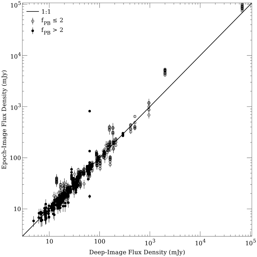
Figure 1.— Comparison between flux densities of cataloged sources as measured in the deep images and those measured in individual epochs. Agreement is generally very good, especially for those sources for which the primary beam correction is not large. The vertical set of points with a large spread corresponds to the highly variable source Cyg X-3. Several sources have a discernable offset between the deep image and epoch flux densities; these are seen in Cyg X-3 pointing, and the offset arises from disagreements between the large-radius behavior of the optimally focused PB model (used to obtain the deep flux density) and that of the defocused PB model (used to open the epoch flux densities). The nominally very bright sources are subject to large, uncertain PB corrections; see §3.6.

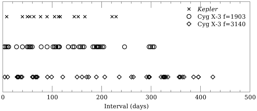
Figure 2.— Intervals between observations for the three sampling patterns present in this work. Different samples are not independent because for $n$ samples there are $n(n-1)/2$ intervals probed. A higher density of measurements around a certain timescale, however, generally indicates increased sensitivity to variability on that timescale.

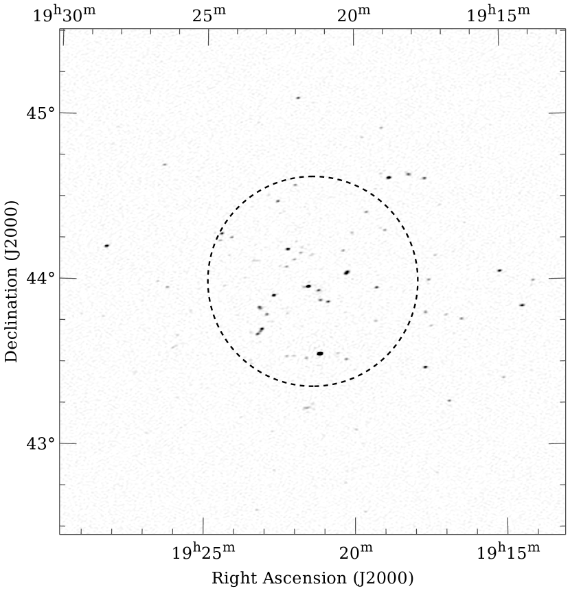
Figure 3.— Deep image of the Kepler pointing, uncorrected for primary beam attenuation. The grayscale is linear from zero (white) to 20 mJy/beam (black). The maximum brightness in the image is $\sim$200 mJy/beam. The rms residual after applying the CLEAN algorithm is 0.5 mJy/beam. The HPBW for this image is 1.27° and is denoted by the dashed circle. The synthesized beam is $65^{\prime\prime}\times 41^{\prime\prime}$ at a position angle of $98\arcdeg$.

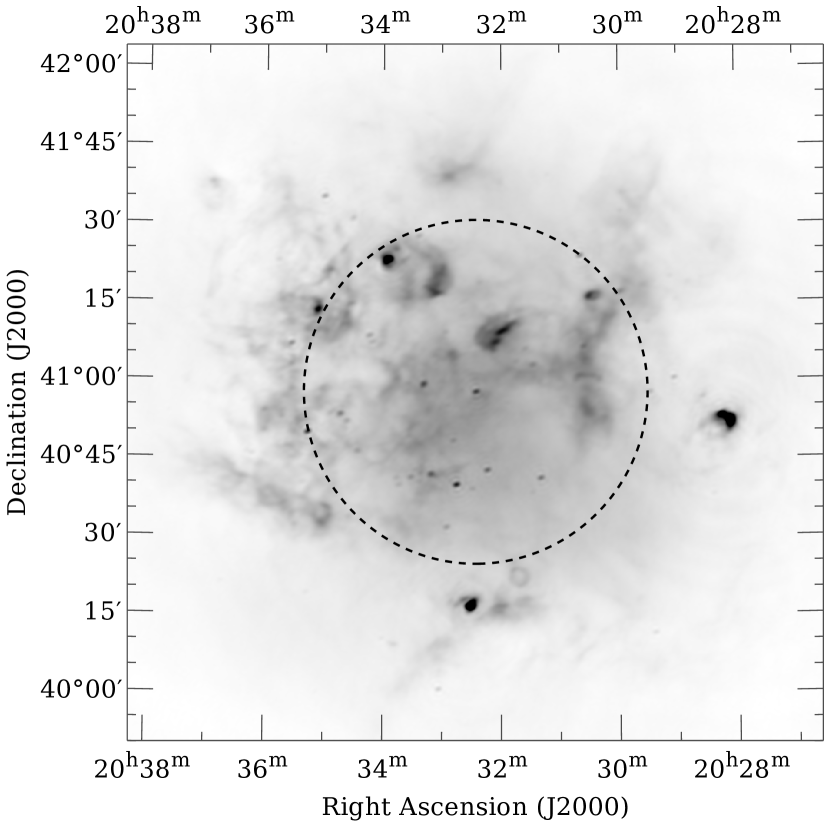
Figure 4.— Deep image of the Cyg X-3 pointing, uncorrected for primary beam attenuation. The grayscale is linear from zero (white) to 150 mJy/beam (black). The maximum brightness in the image is $\sim$500 mJy/beam. The rms deconvolution residual is 1 mJy/beam. A Gaussian prior image was used in the maximum-entropy deconvolution process, causing the restored image to contain emission on angular scales larger than those sampled by the ATA data. The HPBW for this image is 1.1° and is denoted by the dashed circle. The synthesized beam is $60^{\prime\prime}\times 42^{\prime\prime}$ at a position angle of $106\arcdeg$.

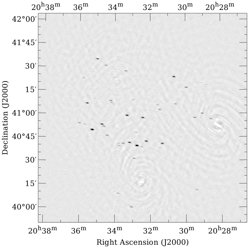
Figure 5.— Image of the Cyg X-3 pointing from 2011 Feb 01 with LSS subtracted. Primary beam correction has not been applied. The grayscale is linear from -5 mJy/beam (white) to 50 mJy/beam (black). (Note that this is different than that used in Figure 4.) The maximum brightness in the image is $\sim$380 mJy/beam. The rms deconvolution residual is 0.9 mJy/beam. The synthesized beam is $85^{\prime\prime}\times 36^{\prime\prime}$ at a position angle of $83\arcdeg$.

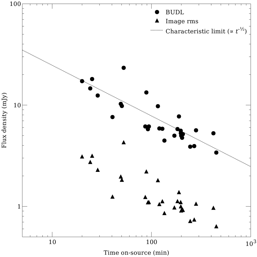
Figure 6.— Noise statistics for epoch images as a function of on-source integration time $t$. Triangles: representative rms values as reported by sfind. Circles: apparent blind unresolved-source detection limits (BUDLs; §4.3). At fixed $t$, achieved values will vary with system temperature, data flagging, calibration quality, and the source detection cutoff dynamically determined by the sfind FDR algorithm. The dashed line shows the characteristic BUDL assuming a scaling of $t^{-1/2}$; for $t=10$ min, this corresponds to $\sim$24 mJy. Both sets of numbers refer to PB-attenuated images and hence apparent flux densities.

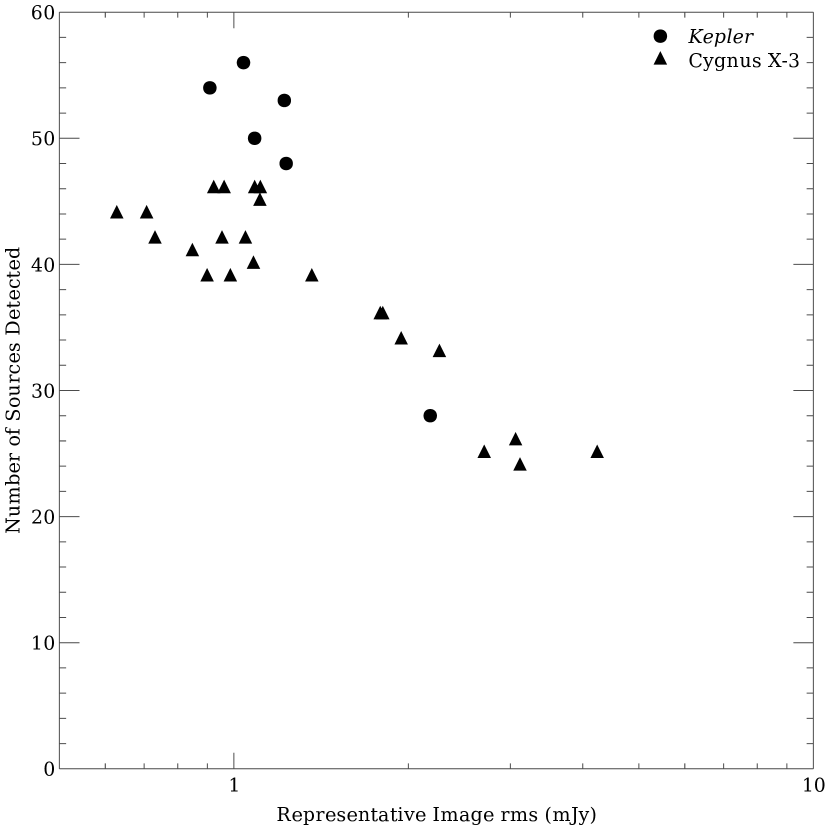
Figure 7.— Number of sources detected in each epoch image, as a function of the representative image rms reported by sfind. Symbols are grouped by pointing. There are 86 cataloged sources associated with the Kepler pointing and 48 with the Cyg X-3 pointing. The detection rate for the Kepler pointing is lower because the Kepler deep image is much less limited by systematics than the Cyg X-3 deep image, and so contains many more faint sources that are cataloged but cannot easily be detected in the epoch images.

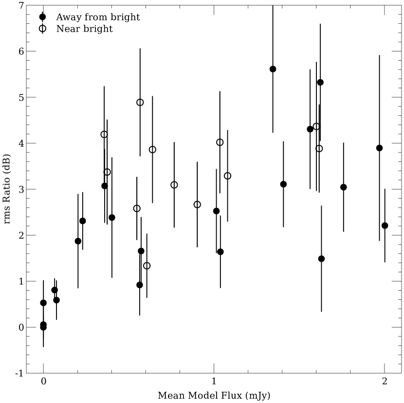
Figure 8.— Measurements of the increase in image noise as a function of LSS flux density. Source-free regions of 50$\times$100 pixels were selected in the Kepler and Cyg X-3 fields. For each epoch image and each region, the rms was computed and divided by the rms in an equally-sized box in the lower left corner of each image, far away from all source emission. Because these values are ratios, they are independent of the primary beam correction. Each plotted point gives the mean and standard deviation of these rms ratios over all imaged epochs for a particular pointing, source-free region, and focus setting. The abscissa is the mean flux density of the LSS model of that region. Open circles denote measurements from regions very near ($\sim$20 pixels) any of the three bright sources of the Cyg X-3 field. Areas in which there is significant LSS show rms increases of a factor of $\sim$2 versus the source-free baseline. See §4.1 for discussion.

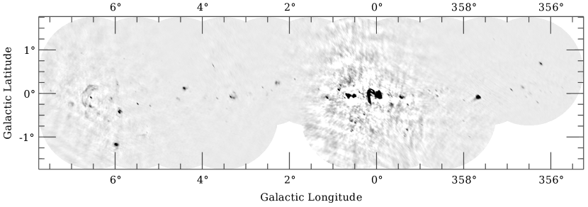
Figure 9.— Preliminary mosaicked image of ASGARD GC field. Unlike the other maps in this paper, a primary beam correction has been applied. The grayscale is linear from -70 mJy/beam (white) to 800 mJy/beam (black). The maximum brightness in the image is $\sim$3920 mJy/beam. Each pointing has been imaged to a diameter of about 2.2 times the HPBW. Most pointings have only a single epoch of observations contributing to the image.

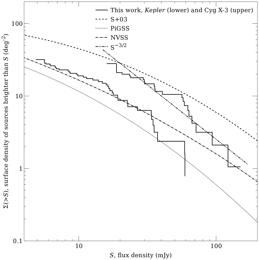
Figure 10.— Cumulative source counts in this and other surveys. ASGARD measurements are derived from the cumulative distribution function of source flux densities as detected in the Kepler and Cyg X-3 deep images, combined with effective search areas based on our analytic primary beam models. Reference values are derived from differential source count measurements reported in S+03, the NVSS (Condon et al., 1998), and PiGSS–I. The arbitrarily-normalized $S^{-3/2}$ line shows the expected scaling for a Euclidean, volume-limited distribution. See §4.2 for discussion.

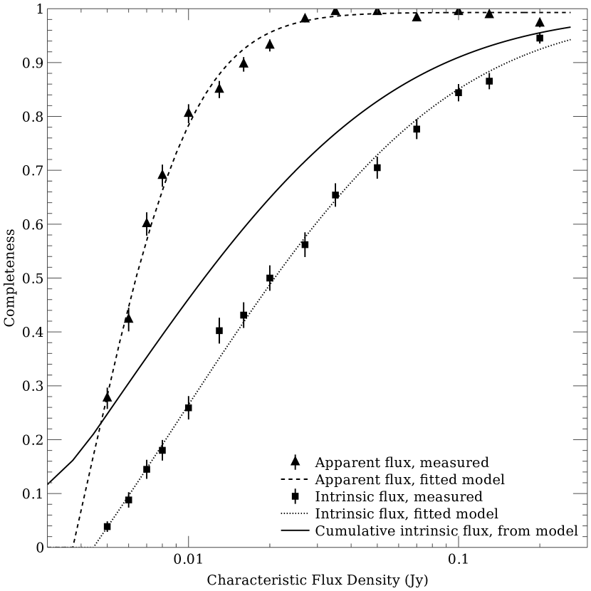
Figure 11.— Completeness of blind source detection in various regimes, as determined from simulations with the current set of epoch images. Apparent completeness measures the detection fraction of sources of a given flux density in images without correction for primary beam attenuation. Intrinsic completeness measures the detection fraction of sources of a single given flux density after correction for PB attenuation. Cumulative intrinsic measures the expected detection fraction for all sources brighter than a given intrinsic flux density, assuming luminosity function $N({>}S)\propto S^{-3/2}$. See §4.3 for discussion.

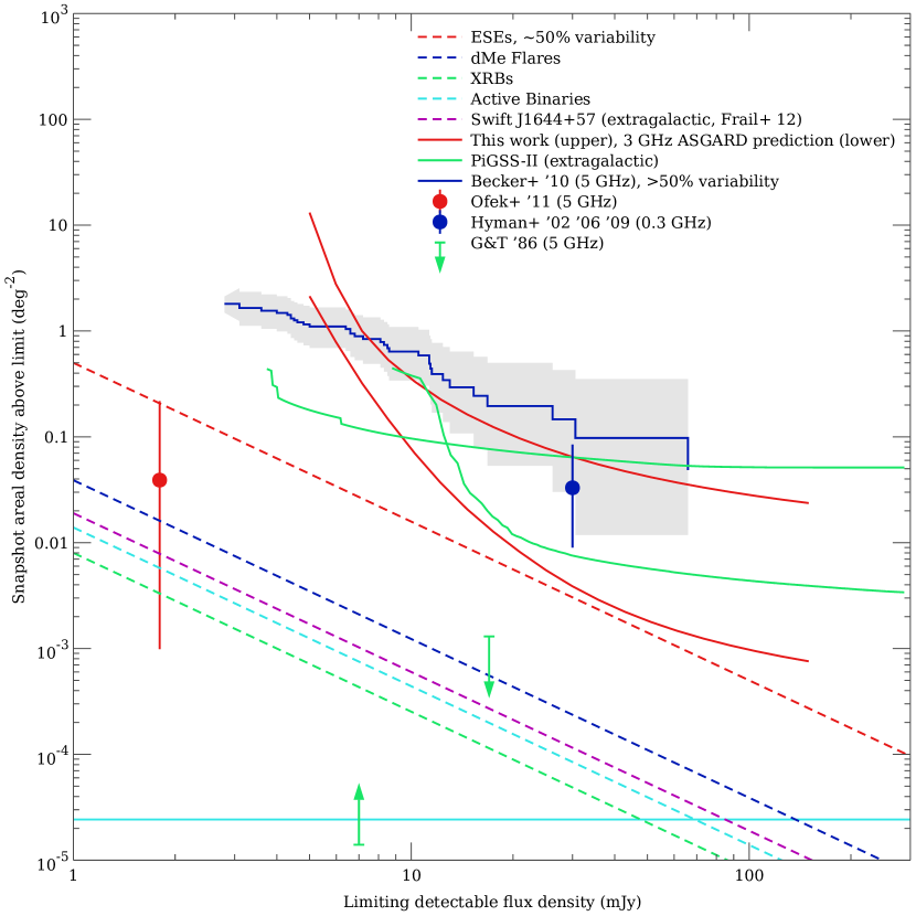
Figure 12.— Measurements of and limits to snapshot areal densities of radio transients. See §5.1 for detailed discussion. All uncertainties are to 95% confidence limit. Upper red line: upper limit on the areal density of Galactic transients from this work alone. Lower red line: predicted upper limit from the complete 3 GHz ASGARD dataset, should no Galactic transients be found. Blue line: areal density of Galactic sources with fractional variability > 50% at 5 GHz on multi-year timescales as measured by Becker et al. (2010). Green lines: extragalactic transient areal density limits from PiGSS–II on daily and monthly timescales. See Bower et al. (2011) for more information. Points and limit arrows: measurements of Galactic transient rates from the VLA at 5 GHz (Ofek et al., 2011), VLA at 0.33 GHz (Hyman et al., 2002, 2006), GMRT at 0.235 GHz (Hyman et al., 2009), and NRAO 91-m transit telescope at 5 GHz (Gregory & Taylor, 1986), as discussed in the text. Dashed lines: areal density estimates for various radio transient populations as discussed in the text. Horizontal line: density corresponding to one event on the whole sky at any given time.

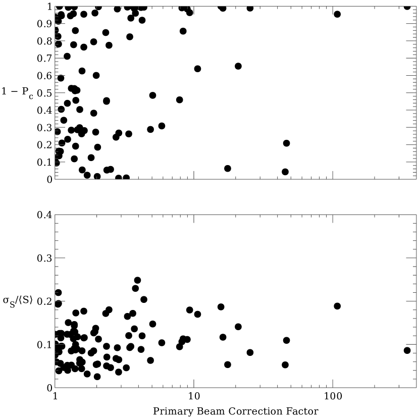
Figure 13.— Variability metrics as a function of primary beam correction factor $f_{\mathrm{PB}}$. The upper panel plots $1-P_{c}$ so that a higher vertical position indicates more variability in both panels. The distributions of the metrics both skew toward higher values as $f_{\mathrm{PB}}$ increases, suggesting less-reliable measurements. Cyg X-3 is omitted from these plots. It has $1-P_{c}\approx 1$ and $\sigma/\langle S\rangle\approx 0.69$.

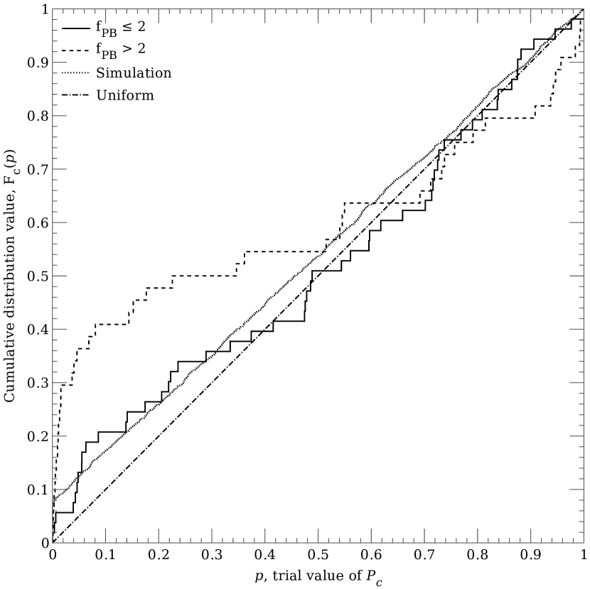
Figure 14.— Cumulative distribution of observed $P_{c}$ values for sources inside and outside the half-power point: given a randomly-chosen source in the dataset, $F_{c}(p)$ is the probability that its $P_{c}$ value is less than $p$. Dash-dotted line: the uniform distribution, $F_{c}(p)=p$, which would be expected in the absence of variability with purely Gaussian errors. Dotted line: simulated observations based on our sampling and a population in which 10% of sources have log-normal flux density variability with a scatter of 0.13 dex. Solid (dashed) line: distribution of values inside (outside) the half-power point. See §4.5 and Appendix A for discussion.

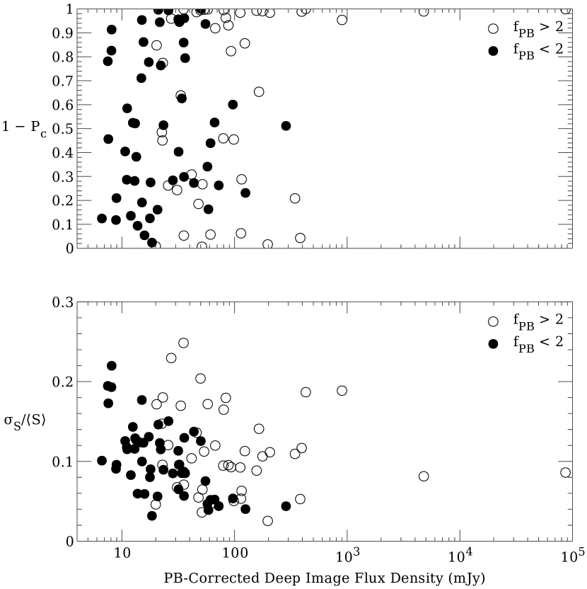
Figure 15.— Variability metrics as a function of deep image flux density. The upper panel plots $1-P_{c}$ so that a higher vertical position indicates more variability in both panels. Among the sources with $f_{\mathrm{PB}}\leq 2$, $\sigma_{S}/\langle S\rangle$ increases for the less reliably-measured faint sources. The quantity $1-P_{c}$ does not show an obvious trend.

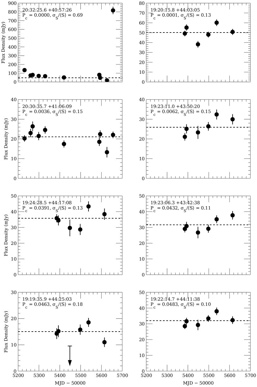
Figure 16.— Lightcurves of the most variable sources in this study. The variability metric $P_{c}$ increases from left to right, top to bottom. (Recall that lower values of $P_{c}$ are associated with higher probabilities of genuine variability.) The most-probably variable source, shown in the top-left panel, is Cyg X-3, here identified as 20:32:25.6 +40:57:26.

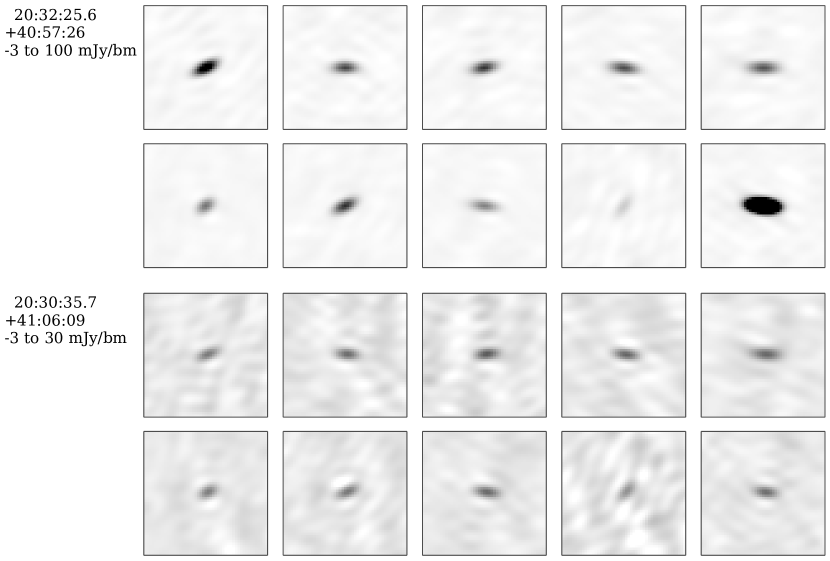
Figure 17.— Image cutouts (in standard J2000 RA/dec. coordinates) of the most variable sources in the Cyg X-3 pointing. Time increases left to right, top to bottom. The coordinates of each source and the bounds of the white-to-black linear intensity scale are annotated to the left of each set of panels. Each panel is 8.2$\times$8.2^′. The top panels show Cyg X-3 itself, here identified as 20:32:25.6 +40:57:26.

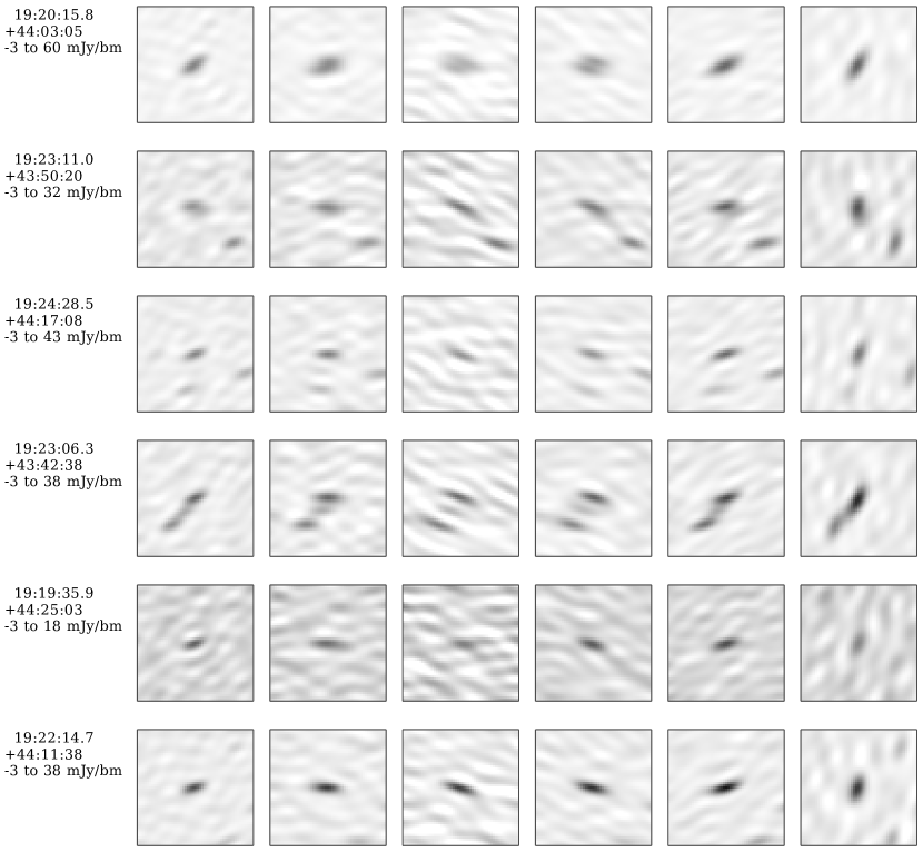
Figure 18.— Image cutouts of the most variable sources in the Kepler pointing. Layout is the same as in Figure 17.

Table 1ASGARD pointing centers and 3 GHz summary statistics.

Field	Identifier	Galactic Coordinates ($\ell$, $b$)				# Epochs	Integ. Time (hr)
GC	gc$-$07$+$1	356.	500	+0.	500	66	45.	29
	gc$-$07$-$1	356.	500	$-$0.	500	0	0.	00
	gc$-$05$+$1	357.	500	+0.	500	66	46.	28
	gc$-$05$-$1	357.	500	$-$0.	500	0	0.	00
	gc$-$03$+$1	358.	500	+0.	500	64	14.	20
	gc$-$03$-$1	358.	500	$-$0.	500	59	10.	84
	gc$-$01$+$1	359.	500	+0.	500	67	14.	72
	gc$-$01$-$1	359.	500	$-$0.	500	76	22.	44
	Sgr A* (catalog )	359.	944	$-$0.	046	3	5.	67
	gc$+$01$+$1	0.	500	+0.	500	70	21.	70
	gc$+$01$-$1	0.	500	$-$0.	500	5	0.	80
	gc$+$03$+$1	1.	500	+0.	500	65	16.	87
	gc$+$03$-$1	1.	500	$-$0.	500	0	0.	00
	gc$+$05$+$1	2.	500	+0.	500	68	15.	92
	gc$+$05$-$1	2.	500	$-$0.	500	0	0.	00
	gc$+$07$+$1	3.	500	+0.	500	33	4.	94
	gc$+$07$-$1	3.	500	$-$0.	500	67	8.	45
	gc$+$09$+$1	4.	500	+0.	500	70	19.	73
	gc$+$09$-$1	4.	500	$-$0.	500	26	2.	48
	gc$+$11$+$1	5.	500	+0.	500	69	11.	33
	gc$+$11$-$1	5.	500	$-$0.	500	3	6.	12
	gc$+$13$+$1	6.	500	+0.	500	72	16.	55
	gc$+$13$-$1	6.	500	$-$0.	500	18	14.	97
Cygnus	Kepler	75.	756	+13.	491	47	96.	72
	Cyg X-3	79.	845	+0.	700	86	153.	05
	x3$+$0$-$2	79.	845	$-$0.	300	13	10.	87
	x3$+$2$+$0	80.	845	+0.	700	20	26.	58
	x3$+$2$-$2	80.	845	$-$0.	300	10	3.	96

Table 2Parameters of ASGARD campaigns.

Subset	Field	Start Date	End Date	# Epochs	Time On-Source (h)
Complete	GC	2009 May 22	2009 Oct 14	64	186
	GC	2010 Mar 01	2010 Oct 21	84	285
	GC	2011 Mar 01	2011 Apr 11	22	54
	Cygnus	2009 Nov 24	2011 Apr 11	159	377
3 GHz	GC	2010 Apr 29	2010 Oct 21	73	245
	GC	2011 Mar 01	2011 Apr 11	22	54
	Cygnus	2010 Feb 03	2011 Apr 11	108	291
This work	Cygnus	2010 Feb 03	2011 Apr 11	30	83

Table 3Eight most variable sources in the ASGARD analysis presented in this work.

R.A.	Decl.	$\langle S\rangle$ (mJy)		$f_{\mathrm{PB}}$		$P_{c}$		$f$		$\sigma_{S}/\langle S\rangle$
20 32 25.6	+40 57 26	47.	5	1.	0	0.	0000	46.	39	0.	69
19 20 15.8	+44 03 05	50.	2	1.	1	0.	0001	1.	58	0.	13
20 30 35.7	+41 06 09	21.	1	1.	4	0.	0036	1.	99	0.	15
19 23 11.0	+43 50 20	25.	9	1.	2	0.	0062	1.	54	0.	15
19 24 28.5	+44 17 08	35.	8	1.	9	0.	0391	1.	51	0.	13
19 23 06.3	+43 42 38	31.	7	1.	4	0.	0432	1.	41	0.	11
19 19 35.9	+44 25 03	15.	0	1.	6	0.	0463	1.	69	0.	18
19 22 14.7	+44 11 38	32.	0	1.	1	0.	0483	1.	33	0.	10

Note. — $\langle S\rangle$ is the weighted mean flux density of the source across all epochs. $f_{\mathrm{PB}}$ is the primary beam correction factor used to determine the intrinsic source flux density. $P_{c}$ is the probability that the source is constant given the measurements, assuming purely Gaussian errors. $f$ is the modulation index of Becker et al. (2010). $\sigma_{S}/\langle S\rangle$ is the modulation index of Ofek et al. (2011). See discussion in §5.2.

References

- Abada-Simon & Aubier (1997) Abada-Simon, M., & Aubier, M. 1997, A&AS, 125, 511
- Baars et al. (1977) Baars, J. W. M., Genzel, R., Pauliny-Toth, I. I. K., & Witzel, A. 1977, A&A, 61, 99
- Bannister et al. (2011a) Bannister, K. W., Murphy, T., Gaensler, B. M., Hunstead, R. W., & Chatterjee, S. 2011a, MNRAS, 412, 634
- Bannister et al. (2011b) —. 2011b, MNRAS, 418, 2813
- Becker et al. (2010) Becker, R. H., Helfand, D. J., White, R. L., & Proctor, D. D. 2010, AJ, 140, 157
- Becker et al. (1995) Becker, R. H., White, R. L., & Helfand, D. J. 1995, ApJ, 450, 559
- Becker et al. (1994) Becker, R. H., White, R. L., Helfand, D. J., & Zoonematkermani, S. 1994, ApJS, 91, 347
- Bell et al. (2011) Bell, M. E., Fender, R. P., Swinbank, J., et al. 2011, MNRAS, 415, 2
- Berger (2002) Berger, E. 2002, ApJ, 572, 503
- Berger et al. (2012) Berger, E., Zauderer, A., Pooley, G. G., et al. 2012, ApJ, 748, 36
- Berger et al. (2001) Berger, E., Ball, S., Becker, K. M., et al. 2001, Nature, 410, 338
- Bhatnagar et al. (2008) Bhatnagar, S., Cornwell, T. J., Golap, K., & Uson, J. M. 2008, A&A, 487, 419
- Birkinshaw (1978) Birkinshaw, M. 1978, MNRAS, 184, 387
- Blair & ATA Team (2009) Blair, S. K., & ATA Team. 2009, BAAS, 41, 670
- Bloom et al. (2011) Bloom, J. S., Giannios, D., Metzger, B. D., et al. 2011, Science, 333, 203
- Bodaghee et al. (2012) Bodaghee, A., Tomsick, J. A., Rodriguez, J., & James, J. B. 2012, ApJ, 744, 108
- Bopp & Fekel (1977) Bopp, B. W., & Fekel, F. 1977, AJ, 82, 490
- Bower et al. (2010) Bower, G., Croft, S., Keating, G., et al. 2010, ApJ, 725, 1792
- Bower et al. (2003) Bower, G. C., Plambeck, R. L., Bolatto, A., et al. 2003, ApJ, 598, 1140
- Bower et al. (2005) Bower, G. C., Roberts, D. A., Yusef-Zadeh, F., et al. 2005, ApJ, 633, 218
- Bower & Saul (2011) Bower, G. C., & Saul, D. 2011, ApJL, 728, L14
- Bower et al. (2007) Bower, G. C., Saul, D., Bloom, J. S., et al. 2007, ApJ, 666, 346
- Bower et al. (2011) Bower, G. C., Whysong, D., Blair, S., et al. 2011, ApJ, 739, 76
- Brinkmann et al. (1997) Brinkmann, W., Siebert, J., Feigelson, E. D., et al. 1997, A&A, 323, 739
- Brogan et al. (2003) Brogan, C. L., Nord, M., Kassim, N., Lazio, J., & Anantharamaiah, K. 2003, Astronomische Nachrichten Supplement, 324, 17
- Broten et al. (1986) Broten, N. W., Vallée, J. P., & MacLeod, J. M. 1986, A&AS, 64, 499
- Brunthaler et al. (2009) Brunthaler, A., Menten, K. M., Reid, M. J., et al. 2009, A&A, 499, L17
- Bulgarelli et al. (2010) Bulgarelli, A., Striani, E., Sabatini, S., et al. 2010, ATel, 2609
- Carilli & Rawlings (2004) Carilli, C., & Rawlings, S. 2004, New A Rev., 48, 979
- Condon et al. (1998) Condon, J. J., Cotton, W. D., Greisen, E. W., et al. 1998, AJ, 115, 1693
- Cordes et al. (2004) Cordes, J. M., Lazio, T. J. W., & McLaughlin, M. A. 2004, New A Rev., 48, 1459
- Cornwell et al. (1999) Cornwell, T., Braun, R., & Briggs, D. S. 1999, in Synthesis Imaging in Radio Astronomy II, ed. G. B. Taylor, C. L. Carilli, & R. A. Perley, Vol. 180, 151
- Cornwell et al. (2008) Cornwell, T. J., Golap, K., & Bhatnagar, S. 2008, IEEE Journal of Selected Topics in Signal Processing, 2, 647
- Cornwell & Perley (1992) Cornwell, T. J., & Perley, R. A. 1992, A&A, 261, 353
- Crocker et al. (2011) Crocker, R. M., Jones, D. I., Aharonian, F., et al. 2011, MNRAS, 413, 763
- Crocker et al. (2010) Crocker, R. M., Jones, D. I., Melia, F., Ott, J., & Protheroe, R. J. 2010, Nature, 463, 65
- Croft et al. (2011) Croft, S., Bower, G. C., Keating, G., et al. 2011, ApJ, 731, 34
- Croft et al. (2010a) Croft, S., Bower, G. C., Ackermann, R., et al. 2010a, ApJ, 719, 45
- Croft et al. (2010b) —. 2010b, ApJ, 724, 827
- Cutri et al. (2012) Cutri, R. M., Wright, E. L., Conrow, T., et al. 2012, Explanatory Supplement to the WISE All-Sky Data Release Products
- Davies et al. (1976) Davies, R. D., Walsh, D., Browne, I. W. A., Edwards, M. R., & Noble, R. G. 1976, Nature, 261, 476
- de Vries et al. (2004) de Vries, W. H., Becker, R. H., White, R. L., & Helfand, D. J. 2004, AJ, 127, 2565
- DeBoer et al. (2009) DeBoer, D. R., Gough, R. G., Bunton, J. D., et al. 2009, IEEE Proc., 97, 1507
- Drake et al. (1989) Drake, S., Simon, T., & Linsky, J. 1989, ApJS, 71, 905
- Eker et al. (2008) Eker, Z., Filiz Ak, N., Bilir, S., et al. 2008, MNRAS, 389, 1722
- Emmanoulopoulos et al. (2010) Emmanoulopoulos, D., McHardy, I. M., & Uttley, P. 2010, MNRAS, 404, 931
- Fanaroff & Riley (1974) Fanaroff, B. L., & Riley, J. M. 1974, MNRAS, 167, 31P
- Favata et al. (1995) Favata, F., Micela, G., & Sciortino, S. 1995, A&A, 298, 482
- Fender & Bell (2011) Fender, R. P., & Bell, M. E. 2011, BASI, 39, 315
- Fiedler et al. (1994a) Fiedler, R., Dennison, B., Johnston, K. J., Waltman, E. B., & Simon, R. S. 1994a, ApJ, 430, 581
- Fiedler et al. (1994b) Fiedler, R., Pauls, T., Johnston, K. J., & Dennison, B. 1994b, ApJ, 430, 595
- Fiedler et al. (1987) Fiedler, R. L., Dennison, B., Johnston, K. J., & Hewish, A. 1987, Nature, 326, 675
- Forbrich et al. (2008) Forbrich, J., Menten, K. M., & Reid, M. J. 2008, A&A, 477, 267
- Fragos et al. (2009) Fragos, T., Kalogera, V., Willems, B., et al. 2009, ApJL, 702, L143
- Frail et al. (2012) Frail, D. A., Kulkarni, S. R., Ofek, E. O., Bower, G. C., & Nakar, E. 2012, ApJ, 747, 70
- Frail et al. (2001) Frail, D. A., Kulkarni, S. R., Sari, R., et al. 2001, ApJL, 562, L55
- Gaensler & Hunstead (2000) Gaensler, B. M., & Hunstead, R. W. 2000, PASA, 17, 72
- Gal-Yam et al. (2006) Gal-Yam, A., Ofek, E. O., Poznanski, D., et al. 2006, ApJ, 639, 331
- Gallo et al. (2012) Gallo, E., Miller, B., & Fender, R. 2012, MNRAS, 423, 590
- Genzel & Townes (1987) Genzel, R., & Townes, C. H. 1987, ARA&A, 25, 377
- Ghosh & Rau (1992) Ghosh, T., & Rau, A. P. 1992, A&A, 264, 203
- Giovanelli et al. (2005) Giovanelli, R., Haynes, M. P., Kent, B. R., et al. 2005, AJ, 130, 2598
- Gray (1994) Gray, A. D. 1994, MNRAS, 270, 861
- Gregory & Kronberg (1972) Gregory, P. C., & Kronberg, P. P. 1972, Nature, 239, 440
- Gregory et al. (1996) Gregory, P. C., Scott, W. K., Douglas, K., & Condon, J. J. 1996, ApJS, 103, 427
- Gregory & Taylor (1986) Gregory, P. C., & Taylor, A. R. 1986, AJ, 92, 371
- Güdel (2002) Güdel, M. 2002, ARA&A, 40, 217
- Gull & Daniell (1978) Gull, S. F., & Daniell, G. J. 1978, Nature, 272, 686
- Hall (1976) Hall, D. S. 1976, in IAU Colloq. 29: Multiple Periodic Variable Stars, ed. W. S. Fitch, Vol. 60, 287
- Hallinan et al. (2007) Hallinan, G., Bourke, S., Lane, C., et al. 2007, ApJL, 663, L25
- Harp et al. (2011) Harp, G. R., Ackermann, R. F., Nadler, Z. J., et al. 2011, IEEE Transactions on Antennas and Propagation, 59, 2004
- Harris & Miley (1978) Harris, D. E., & Miley, G. K. 1978, A&AS, 34, 117
- Hjellming & Han (1995) Hjellming, R. M., & Han, X. 1995, in X-Ray Binaries, ed. W. H. G. Lewin, J. van Paradijs, & E. P. J. van der Heuvel (Cambridge University Press), 308
- Hjellming & Narayan (1986) Hjellming, R. M., & Narayan, R. 1986, ApJ, 310, 768
- Högbom (1974) Högbom, J. A. 1974, A&AS, 15, 417
- Hooper & Goodenough (2011) Hooper, D., & Goodenough, L. 2011, Physics Letters B, 697, 412
- Hopkins et al. (2002) Hopkins, A. M., Miller, C. J., Connolly, A. J., et al. 2002, AJ, 1086
- Hull et al. (2010) Hull, C. L. H., Bower, G. C., Croft, S., et al. 2010, PASP, 122, 1510
- Hyman et al. (2002) Hyman, S. D., Lazio, T. J. W., Kassim, N. E., & Bartleson, A. L. 2002, AJ, 123, 1497
- Hyman et al. (2003) Hyman, S. D., Lazio, T. J. W., Kassim, N. E., Nord, M. E., & Neureuther, J. L. 2003, Astronomische Nachrichten Supplement, 324, 79
- Hyman et al. (2005) Hyman, S. D., Lazio, T. J. W., Kassim, N. E., et al. 2005, Nature, 434, 50
- Hyman et al. (2006) Hyman, S. D., Lazio, T. J. W., Roy, S., et al. 2006, ApJ, 639, 348
- Hyman et al. (2009) Hyman, S. D., Wijnands, R., Lazio, T. J. W., et al. 2009, ApJ, 696, 280
- Jackson et al. (1989) Jackson, P. D., Kundu, M. R., & White, S. M. 1989, A&A, 210, 284
- Jonas (2009) Jonas, J. L. 2009, IEEE Proc., 97, 1522
- Keating et al. (2010) Keating, G., Barott, W., & Wright, M. 2010, Proc. SPIE, 7740, 774016
- Kida et al. (2008) Kida, S., Niinuma, K., Suzuki, S., et al. 2008, New A, 13, 519
- Koch et al. (2010) Koch, D. G., Borucki, W. J., Basri, G., et al. 2010, ApJL, 713, L79
- Körding et al. (2005) Körding, E., Colbert, E., & Falcke, H. 2005, A&A, 436, 427
- Kotani et al. (2011) Kotani, T., Miyazaki, A., Tsuboi, M., et al. 2011, ATel, 3130
- Kraus et al. (2003) Kraus, A., Krichbaum, T. P., Wegner, R., et al. 2003, A&A, 401, 161
- Kuniyoshi et al. (2007) Kuniyoshi, M., Matsumura, N., Takefuji, K., et al. 2007, PASP, 119, 122
- Law et al. (2011a) Law, C. J., Brentjens, M. A., & Novak, G. 2011a, ApJ, 731, 36
- Law et al. (2008) Law, C. J., Yusef-Zadeh, F., & Cotton, W. D. 2008, ApJS, 177, 515
- Law et al. (2011b) Law, C. J., Gaensler, B. M., Bower, G. C., et al. 2011b, ApJ, 728, 57
- Lazio et al. (2000) Lazio, T. J. W., Fey, A. L., Dennison, B., et al. 2000, ApJ, 534, 706
- Levinson et al. (2002) Levinson, A., Ofek, E. O., Waxman, E., & Gal-Yam, A. 2002, ApJ, 576, 923
- Linden et al. (2011) Linden, T., Hooper, D., & Yusef-Zadeh, F. 2011, ApJ, 741, 95
- Lister et al. (2011) Lister, M. L., Aller, M., Aller, H., et al. 2011, ApJ, 742, 27
- Lovell et al. (2008) Lovell, J. E. J., Rickett, B. J., J, et al. 2008, ApJ, 689, 108
- Lutovinov et al. (2007) Lutovinov, A., Revnivtsev, M., Gilfanov, M., & Sunyaev, R. 2007, in The Obscured Universe. Proceedings of the VI INTEGRAL Workshop, ed. S. Grebenev, R. Sunyaev, & C. Winkler (ESA Publication Division), 241
- Marscher & Brown (1975) Marscher, A. P., & Brown, R. L. 1975, ApJ, 200, 719
- Matsumura et al. (2007) Matsumura, N., Daishido, T., Kuniyoshi, M., et al. 2007, AJ, 133, 1441
- Matsumura et al. (2009) Matsumura, N., Niinuma, K., Kuniyoshi, M., et al. 2009, AJ, 138, 787
- McMullin et al. (2007) McMullin, J. P., Waters, B., Schiebel, D., Young, W., & Golap, K. 2007, in Astronomical Data Analysis Software and Systems XVI, ed. R. A. Shaw, F. Hill, & D. J. Bell, Vol. 376, 127
- Migliari & Fender (2006) Migliari, S., & Fender, R. P. 2006, MNRAS, 366, 79
- Morris & Serabyn (1996) Morris, M., & Serabyn, E. 1996, ARA&A, 34, 645
- Muxlow et al. (2010) Muxlow, T. W. B., Beswick, R. J., Garrington, S. T., et al. 2010, MNRAS, 404, L109
- Niinuma et al. (2007) Niinuma, K., Asuma, K., Kuniyoshi, M., et al. 2007, ApJL, 657, L37
- Nishiyama et al. (2010) Nishiyama, S., Hatano, H., Tamura, M., et al. 2010, ApJL, 722, L23
- Noordam & Smirnov (2010) Noordam, J. E., & Smirnov, O. M. 2010, A&A, 524, A61
- Nord et al. (2006) Nord, M. E., Henning, P. A., Rand, R. J., Lazio, T. J. W., & Kassim, N. E. 2006, AJ, 132, 242
- O’Dea & Owen (1985) O’Dea, C. P., & Owen, F. N. 1985, AJ, 90, 927
- Ofek & Frail (2011) Ofek, E. O., & Frail, D. A. 2011, ApJ, 737, 45
- Ofek et al. (2011) Ofek, E. O., Frail, D. A., Breslauer, B., et al. 2011, ApJ, 740, 65
- Osten (2008) Osten, R. 2008, in Bursts, Pulses and Flickering: wide-field monitoring of the dynamic radio sky (Proceedings of Science)
- Owen & Gibson (1978) Owen, F. N., & Gibson, D. M. 1978, AJ, 83, 1488
- Padovani et al. (2007) Padovani, P., Giommi, P., Landt, H., & Perlman, E. 2007, ApJ, 662, 182
- Pen & King (2012) Pen, U. L., & King, L. 2012, MNRAS, 421, L132
- Perley et al. (2011) Perley, R. A., Chandler, C. J., Butler, B. J., & Wrobel, J. M. 2011, ApJL, 739, L1
- Protheroe et al. (2008) Protheroe, R. J., Ott, J., Ekers, R. D., Jones, D. I., & Crocker, R. M. 2008, MNRAS, 390, 683
- Purcell et al. (2008) Purcell, C. R., Hoare, M. G., & Diamond, P. 2008, in Massive Star Formation: Observations Confront Theory, ed. H. Beuther, H. Linz, & T. Henning, Vol. 387, 389
- Rees (1988) Rees, M. J. 1988, Nature, 333, 523
- Rengelink et al. (1997) Rengelink, R. B., Tang, Y., de Bruyn, A. G., et al. 1997, A&AS, 124, 259
- Richards et al. (2003) Richards, M., Waltman, E., Ghigo, F., & Richards, D. 2003, ApJS, 147, 337
- Rickett (1990) Rickett, B. J. 1990, ARA&A, 28, 561
- Rickett et al. (2000) Rickett, B. J., Coles, W. A., & Markkanen, J. 2000, ApJ, 533, 304
- Salter et al. (2008) Salter, D. M., Hogerheijde, M. R., & Blake, G. A. 2008, A&A, 492, L21
- Sault et al. (1995) Sault, R. J., Teuben, P. J., & Wright, M. C. H. 1995, in Astronomical Data Analysis Software and Systems IV, ed. R. A. Shaw, H. E. Payne, & J. J. E. Hayes, Vol. 77, 433
- Sault & Wieringa (1994) Sault, R. J., & Wieringa, M. H. 1994, A&AS, 108, 585
- Schwab (1984) Schwab, F. R. 1984, AJ, 89, 1076
- Setia Gunawan et al. (2003) Setia Gunawan, D. Y. A., de Bruyn, A. G., van der Hucht, K. A., & Williams, P. M. 2003, ApJS, 149, 123
- Simonetti et al. (1985) Simonetti, J. H., Cordes, J. M., & Heeschen, D. S. 1985, ApJ, 296, 46
- Spangler et al. (1989) Spangler, S., Fanti, R., Gregorini, L., & Padrielli, L. 1989, A&A, 209, 315
- Strohmayer et al. (1998) Strohmayer, T., Marshall, F. E., Hjellming, R. M., Rupen, M. P., & Mioduszewski, A. J. 1998, IAU Circ., 6934, 1
- Taylor et al. (1996) Taylor, A. R., Goss, W. M., Coleman, P. H., van Leeuwen, J., & Wallace, B. J. 1996, ApJS, 107, 239
- Taylor & Gregory (1983) Taylor, A. R., & Gregory, P. C. 1983, AJ, 88, 1784
- Thyagarajan et al. (2011) Thyagarajan, N., Helfand, D., White, R., & Becker, R. 2011, ApJ, 742, 49
- Thyagarajan et al. (2012) —. 2012, ApJ, 746, 114
- Tsutsumi et al. (1995) Tsutsumi, T., Gregory, P. C., Duric, N., & Taylor, A. R. 1995, AJ, 110, 238
- Verheijen et al. (2008) Verheijen, M. A. W., Oosterloo, T. A., van Cappellen, W. A., et al. 2008, in The Evolution of Galaxies Through the Neutral Hydrogen Window, ed. R. Minchin & E. Momjian, Vol. 1035, 265
- Waltman et al. (1995) Waltman, E. B., Ghigo, F. D., Johnston, K. J., et al. 1995, AJ, 110, 290
- Weiler et al. (2002) Weiler, K. W., Panagia, N., Montes, M. J., & Sramek, R. A. 2002, ARA&A, 40, 387
- Welch et al. (2009) Welch, J., Backer, D., Blitz, L., et al. 2009, IEEE Proc., 97, 1438
- Wendker et al. (1991) Wendker, H. J., Higgs, L. A., & Landecker, T. L. 1991, A&A, 241, 551
- White et al. (2005) White, R., Becker, R., & Helfand, D. 2005, AJ, 130, 586
- Williams (2010) Williams, P. 2010, in RFI Mitigation Workshop (Proceedings of Science)
- Williams et al. (2012) Williams, P., Law, C., & Bower, G. 2012, PASP, 124, 624
- Williams (2012) Williams, P. K. G. 2012, Allen Telescope Array Memo Series, 89, 1
- Williams et al. (2011) Williams, P. K. G., Tomsick, J. A., Bodaghee, A., et al. 2011, ApJL, 733, L20
- Wright et al. (2010) Wright, E. L., Eisenhardt, P. R. M., Mainzer, A. K., et al. 2010, AJ, 140, 1868
- Wright & Corder (2008) Wright, M., & Corder, S. 2008, SKA Memo Series, 103, 1
- Yusef-Zadeh et al. (1984) Yusef-Zadeh, F., Morris, M., & Chance, D. 1984, Nature, 310, 557
- Zhao et al. (1992) Zhao, J.-H., Roberts, D. A., Goss, W. M., et al. 1992, Science, 255, 1538