How Robust are Linear Sketches to Adaptive Inputs?

Abstract

Linear sketches are powerful algorithmic tools that turn an $n$-dimensional input into a concise lower-dimensional representation via a linear transformation. Such sketches have seen a wide range of applications including norm estimation over data streams, compressed sensing, and distributed computing. In almost any realistic setting, however, a linear sketch faces the possibility that its inputs are correlated with previous evaluations of the sketch. Known techniques no longer guarantee the correctness of the output in the presence of such correlations. We therefore ask: Are linear sketches inherently non-robust to adaptively chosen inputs? We give a strong affirmative answer to this question. Specifically, we show that no linear sketch approximates the Euclidean norm of its input to within an arbitrary multiplicative approximation factor on a polynomial number of adaptively chosen inputs. The result remains true even if the dimension of the sketch is $d=n-o(n)$ and the sketch is given unbounded computation time. Our result is based on an algorithm with running time polynomial in $d$ that adaptively finds a distribution over inputs on which the sketch is incorrect with constant probability. Our result implies several corollaries for related problems including $\ell_{p}$-norm estimation and compressed sensing. Notably, we resolve an open problem in compressed sensing regarding the feasibility of $\ell_{2}/\ell_{2}$-recovery guarantees in presence of computationally bounded adversaries.

1 Introduction

Recent years have witnessed an explosion in the amount of available data, such as that in data warehouses, the internet, sensor networks, and transaction logs. The need to process this data efficiently has led to the emergence of new fields, including compressed sensing, data stream algorithms and distributed functional monitoring. A unifying technique in these fields is the use of linear sketches. This technique involves specifying a distribution $\pi$ over linear maps $A:\mathbb{R}^{n}\rightarrow\mathbb{R}^{r}$ for a value $r\ll n$. A matrix $A$ is sampled from $\pi$. Then, in the online phase, a vector $x\in\mathbb{R}^{n}$ is presented to the algorithm, which maintains the “sketch” $Ax$. This provides a concise summary of $x$, from which various queries about $x$ can be approximately answered. The storage and number of linear measurements (rows of $A$) required is proportional to $r$. The goal is to minimize $r$ to well-approximate a large class of queries with high probability.

Applications of Linear Sketches.

In compressed sensing the goal is to design a distribution $\pi$ so that for $A\sim\pi$, given a vector $x\in\mathbb{R}^{n}$, from $Ax$ one can output a vector $x^{\prime}$ for which $\|x-x^{\prime}\|_{p}\leqslant C\|x_{tail(k)}\|_{q}$, where $x_{tail(k)}$ denotes $x$ with its top $k$ coefficients (in magnitude) replaced with zero, $p$ and $q$ are norms, and $C>1$ is an approximation parameter. The scheme is considered efficient if $r\leqslant k\cdot{\rm poly}(\log n)$. There are two common models, the “for all” and “for each” models. In the “for all” model, a single $A$ is chosen and is required, with high probability, to work simultaneously for all $x\in\mathbb{R}^{n}$. In the “for each” model, the chosen $A$ is just required to work with high probability for any fixed $x\in\mathbb{R}^{n}$.

A related model is the turnstile model for data streams. Here an underlying vector $x\in\mathbb{R}^{n}$ is initialized to $0^{n}$ and undergoes a long sequence of additive updates to its coordinates of the form $x_{i}\leftarrow x_{i}+\delta$. The algorithm is presented the updates one by one, and maintains a summary of what it has seen. If the summary is a linear sketch $Ax$, then given an additive update to the $i$-th coordinate, the summary can be updated by adding $\delta A_{i}$ to $Ax$, where $A_{i}$ is the $i$-th column of $A$. The best known algorithms for any problem in this model maintain a linear sketch. Starting with the work of Alon, Matias, and Szegedy [AMS99], problems such as approximating the $p$-norm $\|x\|_{p}=(\sum_{i=1}^{n}|x_{i}|^{p})^{1/p}$ for $1\leqslant p\leqslant\infty$ (also known as the frequency moments), the heavy hitters or largest coordinates in $x$, and many others have been considered; we refer the reader to [Ind07, Mut05]. Often it is required that the algorithm be able to query the sketch to approximate the statistic at intermediate points in the stream, rather than solely at the end of the stream.

Other examples include distributed computing [MFHH02] and functional monitoring [CMY11]. Here there are $k$ parties $P^{1},\ldots,P^{k}$, e.g., database servers or sensor networks, each with a local stream $\mathcal{S}^{i}$ of additive updates to a vector $x^{i}$. The goal is to approximate statistics, such as those mentioned above, on the aggregate vector $x=\sum_{i=1}^{k}x^{i}$. If the parties share public randomness, they can agree upon a sketching matrix $A$. Then, each party can locally compute $Ax^{i}$, from which $Ax$ can be computed using the linearity of the sketch, namely, $Ax=A(x^{1}+\cdots+x^{k})$. The important measure is the communication complexity, which, since it suffices to exchange the sketches $Ax^{i}$, is proportional to $r$ rather than to $n$.

Adaptively Chosen Inputs.

One weakness with the models above is that they assume the sketching matrix $A$ is independent of the input vector $x$. As pointed out in recent papers [GHR⁺12, GHS⁺12], there are applications for which this is inadequate. Indeed, this occurs in situations for which the result of performing a query on $Ax$ influences future updates to the vector $x$. One example given in [GHR⁺12] is that of a grocery store, in which $x$ consists of transactions, and one uses $Ax$ to approximate the best selling items. The store may update its inventory based on $Ax$, which in turn influences future sales. A more adversarial example given in [GHR⁺12, GHS⁺12] is that of using a compressed sensing radar on a ship to avoid a missile from an attacker. Based on $Ax$, the ship takes evasive action, which is viewed by the attacker, and may change the attack. The matrix $A$ used by the radar cannot be changed between successive attacks for efficiency reasons. Another example arises in high frequency stock trading. Imagine Alice monitors a stream of orders on the stock market and places her own orders depending on statistics based on sketches. A competitor Charlie might have a commercial interest in leading Alice’s algorithm astray by observing her orders and manipulating the input stream accordingly. The question of sketching in adversarial environments was also introduced and motivated in the beautiful work of Mironov, Naor and Segev [MNS08] who provide several examples arising in multiparty sketching applications. Even from a less adversarial point of view, it seems hard to argue that in realistic settings there will be no correlation between the inputs to a linear sketch and previous evaluations of it. Resilience to such correlations would be a desirable robustness guarantee of a sketching algorithm.

A deterministic sketching matrix, e.g., in compressed sensing one that satisfies the “for all” property above, would suffice to handle this kind of feedback. Unfortunately, such sketches provably have much weaker error guarantees. Indeed, if one wants the number $r$ of measurements to be on the order of $k\cdot{\rm poly}(\log n)$, then the best one can hope for is that for all $x\in\mathbb{R}^{n}$, from $Ax$ one can output $x^{\prime}$ for which $\|x-x^{\prime}\|_{2}\leqslant\frac{\varepsilon}{\sqrt{k}}\|x_{tail(k)}\|_{1}$, which is known as the $\ell_{2}/\ell_{1}$ error guarantee. However, if one allows the “for each” property, then there are distributions $\pi$ over sketching matrices $A$ for which for any fixed $x\in\mathbb{R}^{n}$, from $Ax$ one can output $x^{\prime}$ for which $\|x-x^{\prime}\|_{2}\leqslant(1+\varepsilon)\|x_{tail(k)}\|_{2}$ with high probability (over $A\sim\pi$), which is known as the $\ell_{2}/\ell_{2}$ error guarantee. One can verify that the second guarantee is much stronger than the first; indeed, for constant $\varepsilon$ and $k=1$, if $x=(\sqrt{n},\pm 1,\pm 1,\ldots,\pm 1)$, then with the $\ell_{2}/\ell_{1}$ guarantee, an output of $x^{\prime}=0^{n}$ is valid, while for the $\ell_{2}/\ell_{2}$ guarantee, $x^{\prime}_{1}$ must either be large or many coordinates of $x^{\prime}$ must agree in sign with those of $x$.

An important open question, indeed, the first open question in the “Open Questions from the Workshop on Algorithms for Data Streams 2012 at Dortmund”, is whether or not it is possible to achieve the $\ell_{2}/\ell_{2}$ guarantee for probabilistic polynomial time adversaries with limited information about $A$. The weakest possible information an adversary can have about $A$ is through black box queries. Formally, given a sketch $Ax$, there is a function $f(Ax)$ for which its output satisfies a given approximation guarantee with high probability, e.g., in the case of compressed sensing, the guarantee would be that $f(Ax)$ satisfies the $\ell_{2}/\ell_{2}$ guarantee above, while in the case of data streams, the guarantee may be that $f(Ax)=(1\pm\varepsilon)\|x\|_{p}$. The adversary only sees values $f(Ax^{1}),f(Ax^{2}),\ldots,f(Ax^{t})$ for a sequence of vectors $x^{1},\ldots,x^{t}$ of her choice, where $x^{i}$ may depend on $x^{1},\ldots,x^{i-1}$ and $f(Ax^{1}),\ldots,f(Ax^{i-1})$. The goal of the adversary is to find a vector $x$ for which $f(Ax)$ does not satisfy the approximation guarantee. This corresponds to the private model of compressed sensing, given in Definition 3 of [GHS⁺12].

1.1 Our Results

We resolve the above open question in the negative. In fact, we prove a much more general result about linear sketches. All of our results are derived from the following promise problem GapNorm($B$): for an input vector $x\in\mathbb{R}^{n}$, output $0$ if $\|x\|_{2}\leqslant 1$ and output $1$ if $\|x\|_{2}\geqslant B$, where $B>1$ is a parameter. If $x$ satisfies neither of these two conditions, the output of the algorithm is allowed to be $0$ or $1$.

Our main theorem is stated informally as follows.

Theorem 1.1 (Informal version of Theorem 5.13).

There is a randomized algorithm which, given a parameter $B\geqslant 2$ and oracle access to a linear sketch that uses at most $r=n-O(\log(nB))$ rows, with high probability finds a distribution over queries on which the linear sketch fails to solve GapNorm($B$) with constant probability.

The algorithm makes at most ${\rm poly}(rB)$ adaptively chosen queries to the oracle and runs in time ${\rm poly}(rB).$ Moreover, the algorithm uses only $r$ “rounds of adaptivity” in that the query sequence can be partitioned into at most $r$ sequences of non-adaptive queries.

Note that the algorithm in our theorem succeeds on every linear sketch with high probability. In particular, our theorem implies that one cannot design a distribution over sketching matrices with at most $r$ rows so as to output a value in the range $[\|x\|_{2},B\|x\|_{2}]$, that is, a $B$-approximation to $\|x\|_{2}$, and be correct with constant probability on an adaptively chosen sequence of ${\rm poly}(rB)$ queries. This is unless the number $r$ of rows in the sketch is $n-O(\log(nB))$, which agrees with the trivial $r=n$ upper bound up to a low order term. Here $B$ can be any arbitrary approximation factor that is only required to be polynomially bounded in $n$ (as otherwise the running time would not be polynomial). An interesting aspect of our algorithm is that it makes arguably very natural queries as they are all drawn from Gaussian distributions with varying covariance structure.

We also note that the second part of our theorem implies that the queries can be grouped into fewer than $r$ rounds, where in each round the queries made are independent of each other conditioned on previous rounds. This is close to optimal, as if $o(r/\log r)$ rounds were used, the sketching algorithm could partition the rows of $A$ into $o(r/\log r)$ disjoint blocks of $\omega(\log r)$ coordinates, and use the $i$-th block alone to respond to queries in the $i$-th round. If the rows of $A$ were i.i.d. normal random variables, one can show that this would require a super-polynomial (in $r$) number of non-adaptive queries to break, even for constant $B$. Moreover, our theorem gives an algorithm with time complexity polynomial in $r$ and $B$, and therefore rules out the possibility of using cryptographic techniques secure against polynomial time algorithms.

We state our results in terms of algorithms that output any computationally unbounded but deterministic function $f$ of the sketch $Ax.$ However, it is not difficult to extend all of our results to the setting where the algorithm can use additional internal randomness at each step to output a randomized function $f$ of $Ax.$ This is discussed in Section 7.1.

Applications.

We next discuss several implications of our main theorem. Our algorithm in fact uses only query vectors $x$ which are $O(r)$-dimensional for $B\leqslant\exp(r).$ Recall that for such vectors, $\Omega(r^{-1/2}\|x\|_{2})\leqslant\|x\|_{p}\leqslant O(r^{1/2}\|x\|_{2}),$ for all $1\leqslant p\leqslant\infty.$ This gives us the following corollary for any $\ell_{p}$-norm.

Corollary 1.2 (Informal).

No linear sketch with $n-\omega(\log n)$ rows approximates the $\ell_{p}$-norm to within a fixed polynomial factor on a sequence of polynomially many adaptively chosen queries.

The corollary also applies to other problems that are as least as hard as $\ell_{p}$-norm estimation, such as the earthmover distance, or that can be embedded into $\ell_{p}$ with small distortion.

Via a reduction to GapNorm$(B)$, we are able to resolve the aforementioned open question for sparse recovery, even when $k=1$.

Corollary 1.3 (Informal).

Let $C\geqslant 1.$ No linear sketch with $o(n/C^{2})$ rows guarantees $\ell_{2}/\ell_{2}$-recovery on a polynomial number of adaptively chosen inputs. More precisely, we can find with probability $2/3$ an input $x$ for which the output $x^{\prime}$ of the sketch does not satisfy $\|x-x^{\prime}\|_{2}\leqslant C\|x_{\mathrm{tail}(1)}\|_{2}.$

For constant approximation factors $C$, this shows one cannot do asymptotically better than storing the entire input. For larger approximation factors $C$, the dependence of the number of rows on $C$ in this corollary is essentially best possible (at least for small $k$), as we point out in Section 7.3.

Connection to Differential Privacy.

How might one design algorithms that are robust to adversarial inputs? An intriguing approach is offered by the notion of differential privacy [DMNS06]. Indeed, differential privacy is designed to guard a private database $D\in\{0,1\}^{n}$ (here thought of as $n$ private bits) against adversarial and possibly adaptive queries from a data analyst. Intuitively speaking, differential privacy prevents an attacker from reconstructing the private bit string. In our setting we can think of $D$ as the random string that encodes the matrix used by the sketching algorithm and indeed our algorithm is precisely a reconstruction attack in the terminology of differential privacy. It is known that if $D$ is chosen uniformly at random, then after conditioning $D$ on the output of an $\varepsilon$-differentially private algorithm, the string $D$ is a strongly $2\varepsilon$-unpredictable random string [MMP⁺10]. Hence, if the answers given by the sketching algorithm satisfy differential privacy, then the attacker cannot learn the randomness used by the sketching algorithm. This could then be used to argue that the sketch continues to be correct.

An interesting corollary of our work is that it rules out the possibility of correctly answering a polynomial number of “GapNorm queries” using the differential privacy approach outlined above. This stands in sharp contrast to work in differential privacy which shows that a nearly exponential number of adaptive and adversarial “counting queries” can be answered while satisfying differential privacy [RR10, HR10]. A similar (though quantitatively sharper) separation was recently shown for the stateless mechanisms [DNV12] answering counting queries. While linear sketches are stateless, the model we use here in principle permits more flexibility in how the randomness is used by the algorithm so that the previous separation does not apply.

1.2 Comparison to Previous Work

While the above papers [GHR⁺12, GHS⁺12] introduce the problem, the results they obtain do not directly address the general problem. The main result of [GHS⁺12] is that in the private model of compressed sensing, the $\ell_{2}/\ell_{2}$ error guarantee is achievable with $r=k\cdot{\rm poly}(\log n)$ measurements, under the assumption that the algorithm has access to the exact value of $\|x\|_{2}^{2}$ as well as specific Fourier coefficients of $x$ (or approximate values to these quantities that come from a distribution that depends only on the exact values). While in some applications this may be possible, it is not hard to show that this assumption cannot be realized by any linear sketch unless $r\geqslant n$ (nor by any low space streaming algorithm or low communication protocol). The main result in [GHR⁺12] relevant to this problem is that if the adversary can read the sketching matrix $A$, but is required to stream through the entries in a single pass using logarithmic space, then it cannot generate a query $x$ for which the output of the algorithm on $Ax$ does not satisfy the $\ell_{2}/\ell_{2}$ error guarantee. This is quite different from the problem considered here, since we consider multiple adaptively chosen queries rather than a single query, and we do not allow direct access to $A$ but rather only observe $A$ through the outputs $f(Ax^{i})$.

We note that other work has observed the danger of using the output $f(Ax)$ to create an input $x^{\prime}$ for which the value $f(Ax^{\prime})$ is used [AGM12a, AGM12b]. Their solution to this problem is just to use a new sketching matrix $A^{\prime}$ drawn from $\pi$, and instead query $f(A^{\prime}x^{\prime})$. As mentioned, it may not be possible to do this, e.g., if $x^{\prime}$ is a perturbation to $x$, one would need to compute $A^{\prime}x^{\prime}$ without knowing $x^{\prime}$ (since $x$ may only be known through the sketch $Ax$). Other work [IPW11, PW13] has also considered the power of adaptively choosing matrices to achieve fewer measurements in compressed sensing; this is orthogonal to our work since we consider adaptively chosen inputs rather than adaptively chosen sketches.

Sketching in adversarial environments was also the motivation for [MNS08]. However, they consider an adversarial multi-party model that is different from ours.

1.3 Our Techniques and Proof Overview

We prove our main theorem by considering the following game between two parties, Alice and Bob. Alice chooses an $r\times n$ matrix $A$ from distribution $\pi$. Bob makes a sequence of queries $x^{1},\ldots,x^{s}\in\mathbb{R}^{n}$ to Alice, who only sees $Ax^{i}$ on query $i$. Alice responds by telling Bob the value $f(Ax^{i})$. We stress that here $f$ is an arbitrary function here that need not be efficiently computable, but for now we assume that $f$ uses no randomness. This restriction can be removed easily as we show later. Bob’s goal is to learn the row space $R(A)$ of Alice, namely the at most $r$-dimensional subspace of $\mathbb{R}^{n}$ spanned by the rows of $A$. If Bob knew $R(A)$, he could, with probability $1/2$ query $0^{n}$ and with probability $1/2$ query a vector in the kernel of $A$. Since Alice cannot distinguish the two cases, and since the norm in one case is $0$ and in the other case non-zero, she cannot provide a relative error approximation. Our main theorem gives an algorithm (which can be executed efficiently by Bob) that learns $r-O(1)$ orthonormal vectors that are almost contained in $R(A).$ While this does not give Bob a vector in the kernel of $A,$ it effectively reduces Alice’s row space to be constant dimensional thus forcing her to make a mistake on sufficiently many queries.

The conditional expectation lemma.

In order to learn $R(A)$, Bob’s initial query is drawn from the multivariate normal distribution $N(0,\tau I_{n})$, where $\tau I_{n}$ is the covariance matrix, which is just a scalar $\tau$ times the identity matrix $I_{n}$. This ensures that Alice’s view of Bob’s query $x$, namely, the projection $P_{A}x$ of $x$ onto $R(A)$, is spherically symmetric, and so only depends on $\|P_{A}x\|_{2}$. Given $\|P_{A}x\|_{2}$, Alice needs to output $0$ or $1$ depending on what she thinks the norm of $x$ is. The intuition is that since Alice has a proper subspace of $\mathbb{R}^{n}$, she will be confused into thinking $x$ has larger norm than it does when $\|P_{A}x\|_{2}$ is slightly larger than its expectation (for a given $\tau$), that is, when $x$ has a non-trivial correlation with $R(A)$. Formally, we can prove a conditional expectation lemma showing that there exists a choice of $\tau$ for which $\operatorname*{\mathbb{E}}_{x\sim N(0,\tau\mathrm{Id}_{r})}\left[\|P_{A}x\|_{2}^{2}\mid f(Ax)=1\right]-\operatorname*{\mathbb{E}}_{x\sim N(0,\tau\mathrm{Id}_{r})}\left[\|P_{A}x\|_{2}^{2}\right]$ is non-trivially large. This is done by showing that the sum of this difference over all possible $\tau$ in a range $[1,B]$ is noticeably positive. Here $B$ is the approximation factor that we tolerate. In particular, there exists a $\tau$ for which this difference is large. To show the sum is large, for each possible condition $v=\|P_{A}x\|_{2}^{2}$, there is a probability $q(v)$ that the algorithm outputs $1$, and as we range over all $\tau$, $q(v)$ contributes both positively and negatively to the above difference based on $v$’s weight in the $\chi^{2}$-distribution with mean $r\cdot\tau$. The overall contribution of $v$ can be shown to be zero. Moreover, by correctness of the sketch, $q(v)$ must typically be close to $0$ for small values of $v,$ and typically close to $1$ for large values of $v.$ Therefore $q(v)$ zeros out some of the negative contributions that $v$ would otherwise make and ensures some positive contributions in total.

Boosting a small correlation.

Given the conditional expectation lemma we we can find many independently chosen $x^{i}$ for which each $x^{i}$ has a slightly increased expected projection onto Alice’s space $R(A)$. At this point, however, it is not clear how to proceed unless we can aggregate these slight correlations into a single vector which has very high correlation with $R(A).$ We accomplish this by arranging all $m={\rm poly}(n)$ positively labeled vectors $x^{i}$ into an $m\times n$ matrix $G$ and computing the top right singular vector $v^{*}$ of $G.$ Note that this can be done efficiently. We show that, indeed, $\|P_{A}v^{*}\|\geqslant 1-1/{\rm poly}(n).$ In other words $v^{*}$ is almost entirely contained in $R(A).$ This step is crucial as it gives us a way to effectively reduce the dimension of Alice’s space by $1$ as we will see next.

Iterating the attack.

After finding one vector inside Alice’s space, we are unfortunately not done. In fact Alice might initially use only a small fraction of her rows and switch to a new set of rows after Bob learned her initial rows. We thus iterate the previously described attack as follows. Bob now makes queries from a multivariate normal distribution inside of the subspace orthogonal to the the previously found vector. In this way we have effectively reduced the dimension of Alice’s space by $1$, and we can repeat the attack until her space is of constant dimension, at which point a standard non-adaptive attack is enough to break the sketch. Several complications arise at this point. For example, each vector that we find is only approximately contained in $R(A).$ We need to rule out that this approximation error could help Alice. We do so by adding a sufficient amount of global Gaussian noise to our query distribution. This has the effect of making the distribution statistically indistinguishable from a query distribution defined by vectors that are exactly contained in Alice’s space. Of course, we then also need a generalized conditional expectation lemma for such distributions.

Paper Outline

We start with some technical preliminaries in Section 2. We then prove the conditional expectation lemma in Section 4. The proof of this lemma requires rather detailed information about averages of $\chi^{2}$-distributions in certain intervals. The development of these bounds is contained in Section 3. In Section 5 we present and analyze our complete adaptive attack. The proof again requires several technical ingredients. One tool (given in Section 4.2) relates a distance function between two subspaces to the statistical distance of certain distributions that we use in our attack. The other tool in Section 6 analyzes the top singular vector of certain biased Gaussian matrices arising in our attack. In Section 7 we give applications to compressed sensing, data streams, and distributed functional monitoring.

2 Preliminaries

Notation.

Given a subspace $V\subseteq\mathbb{R}^{n},$ we denote by $P_{V}$ the orthogonal projection operator onto the space $V.$ The orthogonal complement of a linear space $V$ is denoted by $V^{\bot}.$ When $X$ is a distribution we use $x\sim X$ to indicate that $x$ is a random variable drawn according to the distribution $X.$

Linear Sketches.

A linear sketch is given by a distribution ${\cal M}$ over $r\times n$ matrices and an evaluation mapping $F\colon\mathbb{R}^{r\times n}\times\mathbb{R}^{r}\to R$ where $R$ is some output space which we typically choose to be $R=\{0,1\}.$ The algorithm initially samples a matrix $A\sim{\cal M}.$ The answer to each query $x\in\mathbb{R}^{n}$ is then given by $F(A,Ax).$ Since the evaluation map $F$ is not restricted in any way, the concrete representation of $A$ as a matrix is not important. We will therefore identify $A$ with its image, an $r$-dimensional subspace of $\mathbb{R}^{n}$ (w.l.o.g. $A$ has full row rank). In this case, we can write an instance of a sketch as a mapping $f\colon\mathbb{R}^{n}\to R$ satisfying the identity $f(x)=f(P_{A}x).$ In this case we may write $f\colon A\to\{0,1\}$ even though $f$ is defined on all of $\mathbb{R}^{n}$ via orthogonal projection onto $A.$

Distributions.

We denote the $d$-dimensional Gaussian distribution with mean $\mu\in\mathbb{R}^{d}$ and independent coordinates with variance $\sigma^{2}\in\mathbb{R}$ by $N(\mu,\sigma^{2})^{d}.$ The statistical distance (or total variation distance) between two distributions $X,Y$ is denoted by $\|X-Y\|_{\mathrm{tv}}.$

3 Certain Averages of $\chi^{2}$-distributions

In this section we develop the main technical ingredients for our conditional expectation lemma. Specifically, we will work in $\mathbb{R}^{d}$ and consider weighted averages of the $\chi^{2}$-distribution in certain intervals. The density function of the squared Euclidean norm of a $d$-dimensional standard Gaussian variable is given by $\nu(s)=s^{d/2-1}e^{-s/2}/2^{d/2}\Gamma(d/2).$ We let $\nu_{\tau,d}\colon[0,\infty)\to[0,1]$ be the density function of a $\chi^{2}$-distribution with $d$-degrees of freedom and expectation $\tau.$ Note that this coincides with the density function of the squared norm of a $d$-dimensional Gaussian variable $N(0,\tau/d)^{d}$ which we will denote as:

$$\nu_{\tau,d}(s)=\frac{d\left(\frac{sd}{\tau}\right)^{d/2-1}e^{-\frac{sd}{2\tau}}}{\tau 2^{d/2}\Gamma(d/2)}\,.$$ (1)

Here we used that $\nu_{\tau,d}(s)=d\nu(sd/\tau)/\tau.$ We will omit the subscript $d$ whenever it is clear from the context. Further, let $\Gamma_{d}$ denote the probability measure on $[0,\infty)$ of the Gamma distribution given by the density $\gamma_{d}\colon(0,\infty)\to[0,1],$

$$\gamma_{d}(x)=\frac{x^{d-1}e^{-x}}{\Gamma(d)}\,.$$ (2)

Lemma 3.1.

Let $0\leqslant a\leqslant b$ and let $s\geqslant 0.$ Then,

$$\int_{a}^{b}s\nu_{\tau}(s)\,\mathrm{d}\tau =\frac{s}{1-2/d}\Gamma_{d/2-1}\left(\left[\frac{sd}{2b},\frac{sd}{2a}\right]\right)$$ (3)

$$\int_{a}^{b}\tau\nu_{\tau}(s)\,\mathrm{d}\tau =\frac{s}{1-6/d+8/d^{2}}\cdot\Gamma_{d/2-2}\left(\left[\frac{sd}{2b},\frac{sd}{2a}\right]\right)\,.$$ (4)

Proof.

Applying Equation 1 and substituting $x=sd/2\tau,$ we have $\frac{\,\mathrm{d}x}{\,\mathrm{d}\tau}=-\frac{sd}{2\tau^{2}}=-\frac{2x^{2}}{sd}\,.$ It follows that $\frac{1}{\tau}\,\mathrm{d}\tau=-\frac{1}{x}\,\mathrm{d}x.$ Put $a^{\prime}=sd/2b$ and $b^{\prime}=sd/2a.$ Thus,

$$\int_{a}^{b}\nu_{\tau}(s)\,\mathrm{d}\tau=\int_{a}^{b}\frac{d\left(\frac{sd}{\tau}\right)^{d/2-1}e^{-\frac{sd}{2\tau}}}{\tau 2^{d/2}\Gamma(d/2)}\,\mathrm{d}\tau=\int_{a^{\prime}}^{b^{\prime}}\frac{dx^{d/2-2}e^{-x}}{2\Gamma(d/2)}\,\mathrm{d}x\,.$$

On the other hand, $\Gamma(d/2)=(d/2-1)\Gamma(d/2-1)\,.$ Hence,

$$\int_{a}^{b}\nu_{\tau}(s)\,\mathrm{d}\tau=\frac{d}{2(d/2-1)}\Gamma_{d/2-1}\left(\left[a^{\prime},b^{\prime}\right]\right)=\left(1+\frac{2}{d-2}\right)\Gamma_{d/2-1}\left(\left[a^{\prime},b^{\prime}\right]\right)\,.$$

The second equation is shown similarly, again substituting $x=sd/2\tau$ and noting that $\,\mathrm{d}\tau=-\frac{sd}{2x^{2}}\,\mathrm{d}x,$

$$\int_{a}^{b}\tau\nu_{\tau}(s)\,\mathrm{d}\tau=\int_{a}^{b}\frac{d\left(\frac{sd}{\tau}\right)^{d/2-1}e^{-\frac{sd}{2\tau}}}{2^{d/2}\Gamma(d/2)}\,\mathrm{d}\tau=\int_{a^{\prime}}^{b^{\prime}}\frac{sd^{2}}{4}\cdot\frac{x^{d/2-3}e^{-x}}{\Gamma(d/2)}\,\mathrm{d}x=\frac{sd^{2}\Gamma_{d/2-2}\left(\left[a^{\prime},b^{\prime}\right]\right)}{4(d/2-1)(d/2-2)}\,.$$

Furthermore,

$$\frac{d^{2}}{4(d/2-1)(d/2-2)}=\frac{1}{4(1/4-1/2d-1/d+2/d^{2})}=\frac{1}{(1-6/d+8/d^{2})}$$

∎

Let us introduce the function $\Delta\colon[0,\infty)\to\mathbb{R}_{\geqslant 0},$ defined as

$$\Delta(s)\stackrel{{\scriptstyle\small\mathrm{def}}}{{=}}\int_{d}^{Bd}(s-\tau)\nu_{\tau}(s)\,\mathrm{d}\tau\,.$$ (5)

Here $B>4$ is some parameter that we will choose later. Figure 1 illustrates the behavior of this function.

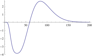
Figure 1: $\Delta(s)$ plotted for $d=20$ and $B=4.$

The next lemma states the properties of $\Delta$ that we will need.

Lemma 3.2.

Assume $d\geqslant 20.$ Then, for every $s\in[0,Bd/2],$ we have that $\Delta(s)<0.$ Moreover, for every $s\in[d,2d],$ we have $\Delta(s)<-s/3d.$

Proof.

First consider the case where $s\in[2d,Bd/2].$ By Lemma 3.1, we have

$$\Delta(s)=\frac{s}{1-2/d}\Gamma_{d/2-1}\left(\left[\frac{s}{2B},\frac{s}{2}\right]\right)-\frac{s}{1-6/d+8/d^{2}}\cdot\Gamma_{d/2-2}\left(\left[\frac{s}{2B},\frac{s}{2}\right]\right)$$

On the other hand, for this choice of $s,$ we have

$$\Gamma_{d/2-2}\left(\left[\frac{s}{2B},\frac{s}{2}\right]\right)\geqslant\Gamma_{d/2-2}\left(\left[\frac{d}{4},d\right]\right)\geqslant 1-1/d$$

Here, the last step can be verified directly by using that $\Gamma_{d/2-2}$ is strongly concentrated around its mean $d/2-2$ and has variance bounded by $\sqrt{d}.$ For $d\geqslant 20,$ the approximation we used is valid. Hence,

$$\Delta(s)\leqslant s\left(\frac{1}{1-2/d}-\frac{1-1/d}{1-6/d+8/d^{2}}\right)=a\left(\frac{1-1/d}{1-3/d+2/d^{2}}-\frac{1-1/d}{1-6/d+8/d^{2}}\right)<-\frac{s}{d}\,.$$

Here we used our lower bound on $d$ again.

Now consider the case $s\in[d-4,2d].$ In this case we have $\Gamma_{d/2-2}([s/2B,s/2])\geqslant\Gamma_{d/2-2}([d/B,d/2-2])\geqslant 1/2-1/d$ by concentration bounds for $\Gamma$ and using that the median of $\Gamma_{d/2-2}$ is at most $d/2-2.$ For the same reason, $\Gamma_{d/2-2}([s/2B,s/2])\geqslant 1/2-1/d.$ Moreover, we have that $\Gamma_{d/2-2}([s/2B,s/2])\geqslant\Gamma_{d/2-1}([s/2B,s/2])$ because $\Gamma_{d/2-1}([d/2-2,\infty))\geqslant\Gamma_{d/2-2}([d/2-2,\infty]).$ This follows because $\Gamma_{d/2-1}$ has larger mean and greater variance than $\Gamma_{d/2-2}.$ Hence,

$$\Delta(s)\geqslant s(1/2-1/d)\left(\frac{1}{1-2/d}-\frac{1}{1-6/d+8/d^{2}}\right)\leqslant-\frac{s}{2d}+\frac{s}{d^{2}}\leqslant-\frac{s}{3d}\,.$$

Finally, let $s\in[0,d-4].$ In this case we have $[s/2B,s/2]\subseteq[0,d/2-2].$ But, for every $x\in[0,d/2-2],$ we have

$$\gamma_{d/2-2}(x)=\gamma_{d/2-1}(x)\left(\frac{d/2-2}{x}\right)\geqslant\gamma_{d/2-1}(x)\,.$$

Hence, $\Delta(s)<0.$

∎

Our main lemma in this section is stated next.

Lemma 3.3.

Let $d\geqslant d_{0}$ for a sufficiently large constant $d_{0}.$ Let $B>4.$ Let $h\colon[0,\infty)\to[0,1]$ be any function satisfying the properties:

1. $\int_{Bd/2}^{2Bd}(1-h(s))\,\mathrm{d}s\leqslant 1/Bd,$

2. $\int_{0}^{2d}h(s)\,\mathrm{d}s\leqslant 1/d.$

Then, we have

$$\int_{s=0}^{\infty}\int_{\tau=l}^{u}(s-\tau)\nu_{\tau}(s)h(s)\,\mathrm{d}\tau\,\mathrm{d}s\geqslant\frac{d}{4}\,.$$ (6)

Proof.

First observe that

$$\int_{s=0}^{\infty}\int_{\tau=l}^{u}(s-\tau)\nu_{\tau}(s)h(s)\,\mathrm{d}\tau\,\mathrm{d}s=\int_{s=0}^{\infty}h(s)\Delta(s)\,\mathrm{d}s$$

Moreover, since $\int_{0}^{\infty}s\nu_{\tau}(s)\,\mathrm{d}s=\tau,$ we have

$$\int_{s=0}^{\infty}\Delta(s)=0\,.$$ (7)

Let us consider the three intervals

$$L=[0,2d),\quad M=[2d,Bd/2),\quad U=[t,\infty).$$

Claim 3.4.

Without loss of generality, $\int_{M}h(s)\Delta(s)\,\mathrm{d}s\geqslant\int_{M}\Delta(s)\,\mathrm{d}s$

Proof.

Lemma 3.2 tells us that $\Delta(s)<0$ for all $s\in M.$ Since we’re interested in lower bounding $\int_{s=0}^{\infty}h(s)\Delta(s),$ we can therefore assume without loss of generality that $h(s)=1$ for all $s\in M.$ ∎

Claim 3.5.

$\int_{U}h(s)\Delta(s)\,\mathrm{d}s\geqslant\int_{U}\Delta(s)\,\mathrm{d}s-6\,.$

Proof.

The claim follows from the first condition on $h$ which implies that $h(s)=1$ almost everywhere in the interval $I=[Bd/2,2Bd].$ In particular,

$$\int_{I}h(s)\Delta(s)\,\mathrm{d}s =\int_{I}\Delta(s)\,\mathrm{d}s+\int_{I}(1-h(s))\Delta(s)\,\mathrm{d}s$$

$$\geqslant\int_{I}\Delta(s)\,\mathrm{d}s-\frac{1}{Bd}\max_{s\in I}|\Delta(s)|\geqslant\int_{I}\Delta(s)\,\mathrm{d}s-4\,.$$

Here we used that $|\Delta(s)|\leqslant 4Bd.$ Moreover, for every $\tau\in[d,Bd]$ we have that $\int_{[2Bd,\infty)}\tau\nu_{\tau}(s)\,\mathrm{d}s\leqslant 1/2Bd$ by standard tail bounds for $\nu_{\tau}$ and sufficiently large $d_{0}.$ This implies

$$\int_{U}h(s)\Delta(s)\,\mathrm{d}s\geqslant\int_{I}h(s)\Delta(s)\,\mathrm{d}s-1\,.$$

Similarly, $\int_{I}\Delta(s)\geqslant\int_{U}\Delta(s)-1.$ The claim follows by combining these statements. ∎

Claim 3.6.

$\int_{L}h(s)\Delta(s)\,\mathrm{d}s\geqslant\int_{L}\Delta(s)+d/3-4.$

Proof.

Here we use the second condition on the claim which implies

$$\int_{L}h(s)\Delta(s)\,\mathrm{d}s\geqslant-\max_{L}|\Delta(s)|\int_{L}h(s)\geqslant-4\,,$$

where we used that $|\Delta(s)|\leqslant 4d$ in this range. On the other hand, by Lemma 3.2, $\Delta(s)<0$ for all $s\in L$ and for $s\in[d,2d]$ we have $\Delta(s)<-s/3d.$ Hence,

$$\int_{L}\Delta(s)\,\mathrm{d}s\leqslant-\frac{1}{3d}\int_{d}^{2d}s\,\mathrm{d}s\leqslant-\frac{d}{3}\,.$$

∎

Combining all three claims we get

$$\int_{0}^{\infty}h(s)\Delta(s)\,\mathrm{d}s\geqslant\int_{0}^{\infty}\Delta(s)\,\mathrm{d}s+\frac{d}{3}-10=\frac{d}{3}-10\,,$$

where we used Equation 7 in the last step. For sufficiently large $d,$ we have $d/3-10\geqslant d/4$ and the lemma follows. ∎

4 Conditional Expectation Lemma

The key tool in our algorithm is what we call the conditional expectation lemma. Informally, it shows that we can always find a distribution over inputs that have a non-trivially large correlation with the unknown subspace used by the linear sketch. Our presentation here, however, will not need the interpretation in terms of linear sketches. Fix a $d$-dimensional linear subspace $U\subseteq\mathbb{R}^{n}.$ Throughout this section, we think of $d$ as being lower bounded by a sufficiently large constant. We will consider functions of the type $f\colon\mathbb{R}^{n}\to\{0,1\}$ which satisfy the identity $f(x)=f(P_{U}x)$ for all $x\in\mathbb{R}^{n}.$ To indicate that this identity holds we will write $f\colon U\to\{0,1\}.$ As explained in Section 2, we can think of these functions as instances of a linear sketch. Our presentation here will not need this fact though.

Definition 4.1 (Subspace Gaussian).

Let $U\subseteq\mathbb{R}^{n}$ be a linear subspace of $\mathbb{R}^{n}.$ We say that a family of distributions ${\cal G}(U)=\{g_{\tau}\}_{\tau\in(0,\infty)}$ is a subspace Gaussian family if

1. $P_{U}g_{\tau}$ is distributed like a standard Gaussian variable inside $U$ satisfying $\operatorname*{\mathbb{E}}\|P_{U}g_{\tau}\|^{2}=\tau.$

2. $P_{U^{\bot}}g_{\tau}$ is a spherical Gaussian distribution that does not depend on $\tau$ and is moreover statistically independent of $P_{U}g_{\tau}.$

Lemma 4.2.

The norm $\|P_{U}g_{\tau}\|^{2}$ is a sufficient statistic for a subspace Gaussian family ${\cal G}(U)=\{g_{\tau}\}_{\tau}.$ Formally, for every $s>0,$ the distribution of $g_{\tau}$ is independent of $\tau$ under the condition that $s=\|P_{U}g_{\tau}\|^{2}.$

Remark 4.3.

The reader concerned about the condition $\|P_{U}g_{\tau}\|^{2}=s$ (which has probability $0$ under $g_{\tau}$) is referred to the excellent article of Chang and Pollard [CP97] (Example 6) where it is shown how to formally justify this conditional distribution using the notion of a disintegration. Specifically, here we mean that the distributions $g_{\tau}$ have a joint disintegration in terms of the variable $\|P_{U}g_{\tau}\|^{2}.$ As explained in [CP97], we can prove the above lemma by appealing to the factorization theorem for sufficient statistics described therein.

Proof of Lemma 4.2.

Note that $g_{\tau}=g_{1}+g_{2}$ where $g_{2}$ is some distribution independent of $\tau$ supported on $U^{\bot}$ and $g_{1}$ is supported on $U.$ By spherical symmetry of both $g_{1}$ and $g_{2}$ we may assume without loss of generality that $U$ is a coordinate subspace, say, the first $d=\dim(U)$ coordinates of the standard basis. Since $g$ is independent of $g_{\tau}$ and supported on a disjoint set of coordinates, it suffices to verify the claim for $g_{1}.$ Specifically, by the Factorization theorem for sufficient statistics (see [CP97]), we need to show that the density of $g_{1}$ can be factored into the product of two functions such $f(x)$ and $h_{\tau}(x)$ that $f$ does not depend on $\tau$ and $h_{\tau}(x)$ depends on $\tau$ but is a function of the parameter $\|x\|^{2}.$ This follows directly from the fact that the Gaussian density at a point $x$ depends only on $\|x\|^{2}.$ ∎

The following definition captures the condition that $f$ should evaluate to $1$ on inputs that have large norm and should evaluate to $0$ on inputs that have small norm.

Definition 4.4 (Soundness).

We say that a function $f\colon U\to\{0,1\}$ is $B$-sound for a subspace Gaussian family ${\cal G}(U),$ where $\dim(U)=d,$ if it satisfies the requirements:

1. $\int_{Bd/2}^{2Bd}\operatorname*{\mathbb{E}}\left[f(g_{\tau})\mid\|P_{U}g_{\tau}\|^{2}=s\right]\,\mathrm{d}s\leqslant 1/Bd\,.$

2. $\int_{0}^{2d}\operatorname*{\mathbb{E}}\left[f(g_{\tau})\mid\|P_{U}g_{\tau}\|^{2}=s\right]\,\mathrm{d}s\leqslant 1/d.$

We are ready to state and prove the Conditional Expectation Lemma.

Lemma 4.5.

Let $B\geqslant 4.$ Let ${\cal G}(U)$ be a subspace Gaussian family where $U$ has dimension sufficiently large dimension $d\geqslant d_{0}.$ Suppose $f\colon U\to\{0,1\}$ is $B$-sound for ${\cal G}(U).$ Then, there exists $\tau\in[d,Bd]$ such that

1. $\operatorname*{\mathbb{E}}\left[\|P_{U}g_{\tau}\|^{2}\,\Big{|}\,f(g_{\tau})=1\right]\geqslant\operatorname*{\mathbb{E}}\left[\|P_{U}g_{\tau}\|^{2}\right]+\frac{1}{4B}$

2. $\operatorname*{\mathbb{P}}\left\{f(g_{\tau})=1\right\}\geqslant\frac{1}{40B^{2}d}\,.$

Proof.

Define the function $h\colon(0,\infty)\to\mathbb{R}$ by putting

$$h(s)=\operatorname*{\mathbb{E}}\left[f(g_{\tau})\mid\|P_{U}g_{\tau}\|^{2}=s\right]\,.$$ (8)

Note that this is well-defined by Lemma 4.2. Let us first rewrite the conditional expectation as follows.

$$\operatorname*{\mathbb{E}}\left[\|P_{U}g_{\tau}\|^{2}\,\Big{|}\,f(g_{\tau})=1\right] =\int_{0}^{\infty}s\operatorname*{\mathbb{P}}\left\{\|P_{U}g_{\tau}\|^{2}=s\mid f(g_{\tau})=1\right\}\,\mathrm{d}s$$

$$=\int_{0}^{\infty}s\operatorname*{\mathbb{P}}\left\{f(g_{\tau})=1\mid\|P_{U}g_{\tau}\|^{2}=s\right\}\cdot\frac{\nu_{\tau}(s)}{\operatorname*{\mathbb{P}}\left\{f(g_{\tau})=1\right\}}\,\mathrm{d}s$$ (by Bayes’ rule)

$$=\int_{0}^{\infty}\frac{sh(s)\nu_{\tau}(s)}{\operatorname*{\mathbb{P}}\left\{f(g_{\tau})=1\right\}}\,\mathrm{d}s$$

Note that here and in the following $\nu_{\tau}=\nu_{\tau,d},$ i.e., the $\chi^{2}$-distribution has $d$ degrees of freedom corresponding to the dimension of $U.$

Claim 4.6.

The lemma follows from follows from the following inequality:

$$\int_{l}^{u}\int_{0}^{\infty}(s-\tau)\nu_{\tau}(s)h(s)\,\mathrm{d}s\,\mathrm{d}\tau\geqslant\frac{d}{4}.$$ (9)

Proof.

Indeed, assuming the above inequality, it follows that there must be a $\tau\in[d,Bd]$ such that

$$\int_{0}^{\infty}s\nu_{\tau}(s)h(s)\,\mathrm{d}s\geqslant\tau\int_{0}^{\infty}\nu_{\tau}(s)h(s)\,\mathrm{d}s+\frac{d}{4Bd}=\tau\operatorname*{\mathbb{P}}\left\{f(g_{\tau})=1\right\}+\frac{1}{4B}\,.$$

In particular,

$$\operatorname*{\mathbb{E}}\left[\|P_{U}g_{\tau}\|^{2}\,\Big{|}\,f(g_{\tau})=1\right]=\int_{0}^{\infty}\frac{sh(s)\nu_{\tau}(s)}{\operatorname*{\mathbb{P}}\left\{f(g_{\tau})=1\right\}}\,\mathrm{d}s\geqslant\frac{\tau\operatorname*{\mathbb{P}}\left\{f(g_{\tau})=1\right\}+1/4B}{\operatorname*{\mathbb{P}}\left\{f(g_{\tau})=1\right\}}\geqslant\tau+\frac{1/4B}{\operatorname*{\mathbb{P}}\left\{f(g_{\tau})=1\right\}}.$$

Since $\operatorname*{\mathbb{P}}\left\{f(g_{\tau})=1\right\}\leqslant 1,$ this gives us the first conclusion of the lemma. It remains to lower bound $\operatorname*{\mathbb{P}}\left\{f(g_{\tau})=1\right\}.$ Here we use that $\int_{5Bd}^{\infty}s\nu_{\tau}(s)h(s)\,\mathrm{d}s\leqslant\frac{1}{2}\int_{0}^{\infty}s\nu_{\tau}(s)h(s)\,\mathrm{d}s,$ by standard concentration properties of $\nu_{\tau}.$ Hence,

$$\operatorname*{\mathbb{P}}\left\{f(g_{\tau})=1\right\}=\int_{0}^{\infty}\nu_{\tau}(s)h(s)\,\mathrm{d}s\geqslant\frac{1}{10Bd}\int_{0}^{\infty}s\nu_{\tau}(s)h(s)\,\mathrm{d}s\geqslant\frac{1/4B}{10Bd}=\frac{1}{40B^{2}d}\,.$$

∎

By the previous claim, it suffices to prove Equation 9. To do so we will apply Lemma 3.3. The lemma in fact directly implies the claim, if we can show that $h$ satisfies the properties required in Lemma 3.3. It is easily verified that these properties coincide with the soundness assumption on $f.$ Thus,

$$\int_{l}^{u}\int_{0}^{\infty}(s-\tau)\nu_{\tau}(s)h(s)\,\mathrm{d}s\,\mathrm{d}\tau\geqslant\frac{d}{3}-2\geqslant\frac{d}{4}\,.$$

This concludes the proof of Lemma 4.5. ∎

The following corollary is a direct consequence of Lemma 4.5 that states that there is one direction in the subspace that has increased variance.

Corollary 4.7.

Let ${\cal G}(U)$ satisfy the assumptions of Lemma 4.5. Then, there is $\tau\in[d,Bd]$ and a vector $u\in U,$ satisfying,

1. $\operatorname*{\mathbb{E}}\left[\langle u,g_{\tau}\rangle^{2}\,\Big{|}\,f(g_{\tau})=1\right]\geqslant\operatorname*{\mathbb{E}}\left[\langle u,g_{\tau}\rangle^{2}\right]+\frac{1}{4Bd}$

2. $\operatorname*{\mathbb{P}}\left\{f(g_{\tau})=1\right\}\geqslant\frac{1}{40B^{2}d}\,.$

Proof.

Pick an arbitrary orthonormal basis $u_{1},\dots,u_{d}$ of $U.$ Since $\|P_{U}g_{\tau}\|^{2}=\sum_{i=1}^{d}\langle u_{i},g_{\tau}\rangle^{2},$ one of the basis vectors must satisfy the conclusion of the lemma by an averaging argument. ∎

4.1 Noisy orthogonal complements

In this section we extend the conditional expectation lemma to a family of distributions that will be important to us later on. We will fix a $r$-dimensional subspace $A\subseteq\mathbb{R}^{n}.$ The family of distributions we will define next isn’t subspace Gaussian on $A,$ but rather subspace Gaussian on $A\cap V^{\bot},$ where $V\subseteq A$ is a linear subspace of $A$ of dimension $\dim(V)\leqslant d-1.$

A distribution in this family is given by a subspace $V$ and a variance $\sigma^{2}.$ Intuitively, the distribution corresponds to a Gaussian distribution on the subspace $V^{\bot}$ of variance $\sigma^{2}$ plus a small Gaussian supported on all of $\mathbb{R}^{n}$ of constant variance independent of $\sigma^{2}.$ The formal definition is given next.

Definition 4.8.

Let $\sigma>0.$ Given a subspace $V\subseteq A$ of dimension $t\leqslant r-1$ and let $d=r-t.$ We define the distribution $G(V^{\bot},\sigma^{2})$ as the distribution obtained from sampling $g_{1}\sim N(0,\sigma^{2})^{n},g_{2}\sim N(0,1/4)^{n}$ independently outputting $g=P_{V^{\bot}}g_{1}+g_{2}.$

Further we define the family of distributions ${\cal G}(A\cap V^{\bot})=\{g_{\tau}\}$ by letting $g_{\tau}=P_{A}g$ where $g\sim G(V^{\bot},\tau/d-1/4)$ if $\tau/d>1/4$ and otherwise we put $g_{\tau}=P_{A}g$ where $g\sim N(0,\tau/d)^{n}$ otherwise.

The next lemma confirms that ${\cal G}(A\cap V^{\bot})$ is subspace Gaussian.

Lemma 4.9.

${\cal G}(A\cap V^{\bot})$ is a subspace Gaussian family.

Proof.

Let $U=A\cap V^{\bot}.$ For $\tau\leqslant 1/4,$ it is clear that $\operatorname*{\mathbb{E}}\|P_{U}g_{\tau}\|^{2}=d\tau/d=\tau$ as is required and $\|P_{U^{\bot}}g_{\tau}\|=0.$ For $\tau>1/4,$ recall that $g=P_{V^{\bot}}g_{1}+g_{2}.$ Hence, inside $P_{U}g$ is distributed like a spherical Gaussian with variance $\tau/d$ in each direction. In particular,

$$\|P_{U}g_{\tau}\|^{2}=\|P_{U}(g_{1}+g_{2})\|^{2}=d\tau/d=\tau\,.$$

On the other hand, $P_{U^{\bot}}g$ only depends on $g_{2}$ and is hence independent of $\tau.$ This shows the second property of subspace Gaussian. ∎

The next definition captures the correctness requirement on $f$ for inputs drawn from the distribution $G(V^{\bot},\sigma^{2}).$

Definition 4.10 (Correctness).

We say that a function $f\colon A\to\{0,1\}$ is $(\varepsilon,B)$-correct on $V^{\bot}$ with $d=\dim(V^{\bot}\cap A)$ if:

1. for all $\sigma^{2}\in[B/2,2B]$ and $g\sim G(V^{\bot},\sigma^{2})$ we have $\operatorname*{\mathbb{P}}\left\{f(g)=1\right\}\geqslant 1-\varepsilon$

2. for all $\sigma^{2}\in[0,2]$ and $g\sim G(V^{\bot},\sigma^{2})$ we have $\operatorname*{\mathbb{P}}\left\{f(g)=1\right\}\leqslant\varepsilon.$

We say that $f$ is $B$-correct on $V^{\bot}$ if it is $(\varepsilon,B)$-correct for some $\varepsilon\leqslant 1/10(Bd)^{2}.$

We will now relate the correctness definition to our earlier soundness definition.

Lemma 4.11.

If $f$ is $B$-correct on $V^{\bot},$ then $f$ is $B$-sound for ${\cal G}(A\cap V^{\bot}).$

Proof.

We will prove the claim in its contrapositive. Indeed suppose that $f$ is not $B$-sound for ${\cal G}(A\cap V^{\bot}).$ This means that one of the two requirements in Definition 4.4 is not satisfied. Suppose it is the first one. In this case we know that for $I=[Bd/2,2Bd]$ and $h(s)=\operatorname*{\mathbb{P}}\left\{f(g_{\tau})=1\mid\|g_{\tau}\|^{2}=s\right\},$ we have $\operatorname*{\mathbb{E}}_{s\in I}(1-h(s))>1/2(Bd)^{2}.$ Suppose we sample $g\sim G(V^{\bot},\sigma^{2})$ where $\sigma^{2}$ is chosen uniformly at random from $B/2,2B.$ We claim that that the distribution of $\|g\|^{2}$ is pointwise within a factor $5$ of the uniform distribution inside the interval $[B/2,2B].$ Hence, $\operatorname*{\mathbb{E}}h(\|g\|^{2})>1/10(Bd)^{2}.$ This violates the first condition of correctness.

The case where the second requirement of Definition 4.4 is violated follows from an analogous argument. ∎

Below we state a variant of the conditional expectation lemma for distributions of the above form. Moreover, we will remove the requirement that $t\leqslant r-d_{0}$ and obtain a result that applies to any $t\leqslant\dim(A).$

Lemma 4.12.

Let $A\subseteq\mathbb{R}^{n}$ be a subspace of dimension $\dim(A)=r\leqslant n-d_{0}$ for some sufficiently large constant $d_{0}.$ Let $V\subseteq A$ be a subspace of $A$ of dimension $t\leqslant r.$ Suppose that $f\colon A\to\{0,1\}$ is $(1/10(d_{0}B)^{2},B)$-correct on $V^{\bot}.$ Then, there exists a scalar $\sigma^{2}\in[3/4,B],$ and a vector $u\in A\cap V^{\bot}$ such that for $g\sim G(V^{\bot},\sigma^{2})$ we have for $d=\max\{r-d,d_{0}\}:$

1. $\operatorname*{\mathbb{E}}\left[\langle u,g\rangle^{2}\,\Big{|}\,f(g)=1\right]\geqslant\operatorname*{\mathbb{E}}\left[\langle u,g\rangle^{2}\right]+\frac{1}{4Bd}$

2. $\operatorname*{\mathbb{P}}\left\{f(g)=1\right\}\geqslant\frac{1}{40B^{2}d}\,.$

Proof.

Before we proceed we would like to ensure that $\dim(A\cap V^{\bot})$ is at least a sufficiently large constant $d_{0}.$ This can be ensured without loss of generality by considering instead a subspace $A^{\prime}\supseteq A$ of dimension $r+d_{0}$ obtained by extending $A$ arbitrarily to $r+d_{0}$ dimensions. This can be done since $n\geqslant r+d_{0}.$ Define the function $f^{\prime}(x)=f(P_{A}x).$ Note that $f^{\prime}(x)=f(x)$ on all $x\in\mathbb{R}^{n}.$ Hence, $f^{\prime}$ is still $(1/10(d_{0}B)^{2},B)$-correct on $V^{\bot}.$ Moreover, now $\dim(V^{\bot}\cap A)=d_{0}.$ Hence, by Lemma 4.11, we have that $f$ is sound for the subspace Gaussian family ${\cal G}(A^{\prime}\cap V^{\bot}).$ Let $U=A^{\prime}\cap V^{\bot}.$ We can apply Corollary 4.7 to ${\cal G}(U)$ to conclude that there is $\tau\in[d,Bd]$ and $u\in U$ such that

$$\operatorname*{\mathbb{E}}\left[\langle u,g_{\tau}\rangle^{2}\,\Big{|}\,f^{\prime}(g_{\tau})=1\right]\geqslant\operatorname*{\mathbb{E}}\left[\langle u,g_{\tau}\rangle^{2}\right]+\frac{1}{4Bd}$$

and $\operatorname*{\mathbb{P}}\left\{f^{\prime}(g_{\tau})=1\right\}\geqslant\frac{1}{40B^{2}d}\,.$ By definition of $f^{\prime}$ the condition $f^{\prime}(g_{\tau})=1$ is equivalent to $f(g_{\tau})=1.$ The condition $f(g_{\tau})=1$ does not affect any vector that is orthogonal to $A.$ Hence we may assume that $u\in A\cap V^{\bot}.$ Also note that $g_{\tau}=P_{A^{\prime}}g$ for some $g\sim G(V^{\bot},\sigma^{2})$ with $\sigma^{2}\in[3/4,B].$ Moreover, $f(g)=f^{\prime}(g_{\tau}),$ and also $\langle u,g_{\tau}\rangle=\langle u,g\rangle$ since $u\in U.$ Hence, we have

$$\operatorname*{\mathbb{E}}\left[\langle u,g\rangle^{2}\,\Big{|}\,f(g)=1\right]\geqslant\operatorname*{\mathbb{E}}\left[\langle u,g\rangle^{2}\right]+\frac{1}{4Bd}$$

with $\operatorname*{\mathbb{P}}\left\{f(g)=1\right\}\geqslant\frac{1}{40B^{2}d}\,.$ This is what we wanted to show. ∎

4.2 Distance between subspaces

Our goal is to relate distributions of the form $G(V^{\bot},\sigma^{2})$ to $G(W^{\bot},\sigma^{2})$ where $V$ and $W$ are subspaces. For this purpose, we consider the following distance function $d(V,W)$ between two subspaces $V,W\subseteq\mathbb{R}^{n}:$

$$d(V,W)=\|P_{V}-P_{W}\|_{2}=\sup_{v\in\mathbb{R}^{n}}\frac{\|P_{V}v-P_{W}v\|}{\|v\|}\,.$$ (10)

We will show that if $V$ and $W$ are close in this distance measure, then the two distributions $G(V^{\bot},\sigma^{2})$ and $G(W^{\bot},\sigma^{2})$ are statistically close. Recall that we denote the statistical distance between two distributions $X,Y$ by $\|X-Y\|_{\mathrm{tv}}.$ We need the following well-known fact.

Fact 4.13.

Let $v\in\mathbb{R}^{n}.$ Then,

$$\|N(0,\sigma^{2})^{n}-N(v,\sigma^{2})^{n}\|_{\mathrm{tv}}\leqslant\frac{\|v\|}{\sigma}\,.$$

Using this fact we can express the statistical distance between $G(V^{\bot},\sigma^{2})$ and $G(W^{\bot},\sigma^{2})$ for two subspaces $V,W$ in terms of the distance $d(V,W).$

Lemma 4.14.

For every $\sigma^{2}\in(0,B],$ we have

$$\|G(V^{\bot},\sigma^{2})-G(W^{\bot},\sigma^{2})\|_{\mathrm{tv}}\leqslant 20\sqrt{Bn\log(Bn)}\cdot d(V,W)+\frac{1}{(Bn)^{5}}\,.$$

Proof.

Sample $g_{1}\sim N(0,\sigma^{2})^{n}$ and $g_{2},g_{2}^{\prime}\sim N(0,1/4)^{n}$ independently. Let us denote by $x=P_{V^{\bot}}g_{1}+g_{2}$ and by $y=P_{W^{\bot}}g_{1}+g_{2}^{\prime}.$ Note that $x$ is distributed like a random draw from $G(V^{\bot},\sigma^{2})$ and $y$ like a draw from $G(W^{\bot},\sigma^{2}).$ However, we introduced a dependence throw $g_{1}.$ Note that it is sufficient to bound the statistical distance of these coupled variables. On the one hand,

$$\|P_{V^{\bot}}g_{1}-P_{W^{\bot}}g_{1}\|=\|P_{V}g_{1}-P_{W}g_{1}\|\leqslant\|g_{1}\|\cdot d(V,W)$$

On the other hand, by Gaussian concentration bounds,

$$\operatorname*{\mathbb{P}}\left\{\|g_{1}\|\leqslant 10\sqrt{Bn\log(Bn)}\right\}\leqslant\frac{1}{(Bn)^{5}}\,.$$

Condition on $\|g_{1}\|\leqslant 10\sqrt{Bn\log(Bn)}.$ Under this condition, for every possible value $u=P_{V^{\bot}}g_{1}-P_{W^{\bot}}g_{1},$ we have

$$\|N(u,1/4)^{n}-N(0,1/4)^{n}\|_{\mathrm{tv}} \leqslant 2\|u\|$$ (by Fact 4.13)

$$\leqslant 2\|g_{1}\|\cdot d(V,W)\leqslant 20\sqrt{Bn\log(Bn)}\cdot d(V,W)\,.$$

Noting that $u+N(0,1/4)^{n}=N(u,1/4)^{n},$ it follows

$$\|P_{V}^{\bot}g_{1}+N(0,1/4)^{n}-P_{W}^{\bot}g_{1}+N(0,1/4)^{n}\|_{\mathrm{tv}} =\|N(u,1/4)^{n}-N(0,1/4)^{n}\|_{\mathrm{tv}}$$

$$\leqslant 20\sqrt{Bn\log(Bn)}\cdot d(V,W)\,.$$

Finally, since the condition $\|g_{1}\|\leqslant 10\sqrt{Bn\log(Bn)}$ has probability $1-1/(Bn)^{5},$ removing it can only increase the statistical distance of the two variables by additive $1/(Bn)^{5}.$ ∎

5 An Adaptive Reconstruction Attack

We next state and prove our main theorem. It shows that no function $f\colon\mathbb{R}^{n}\to\{0,1\}$ that depends only on a lower dimensional subspace can correctly predict the $\ell_{2}^{2}$-norm up to a factor $B$ on a polynomial number of adaptively chosen inputs. Here, $B$ can be any factor and the complexity of our attack will depend on $B$ and the dimension of the subspace. We will in fact show a more powerful distributional result. This result states that no such function can predict the $\ell_{2}^{2}$-norm on a rather natural sequence of distributions even if we allow the function to err on each distribution with inverse polynomial probability. This distributional strengthening will be useful in our application to compressed sensing later on. The next definition formalizes the way in which a linear sketch will fail under our attack.

Definition 5.1 (Failure certificate).

Let $B\geqslant 8$ and let $f\colon\mathbb{R}^{n}\to\{0,1\}.$ We say that a pair $(V,\sigma^{2})$ is a $d$-dimensional failure certificate for $f$ if $V\subseteq\mathbb{R}^{n}$ is $d$-dimensional subspace and $\sigma^{2}\in[0,2B]$ such that for some constant $C>0,$ we have $n\geqslant d+10C\log(Bn)$ and moreover:

• Either $\sigma^{2}\in[B/2,50B]$ and $\operatorname*{\mathbb{P}}_{g\sim G(V^{\bot},\sigma^{2})}\left\{f(g)=1\right\}\leqslant 1-(Bn)^{-C},$

• or $\sigma^{2}\leqslant 2$ and $\operatorname*{\mathbb{P}}_{g\sim G(V^{\bot},\sigma^{2})}\left\{f(g)=1\right\}\geqslant n^{-C}.$

The motivation for the previous definition is given by the next simple fact showing that a failure certificate always gives rise to a distribution over which $f$ does not decide the GapNorm problem up to a factor $\Omega(B)$ on a polynomial number of queries. We note that in Section 5.3 we strengthen this concept to give a distribution where $f$ errs with constant probability.

Fact 5.2.

Given a $d$-dimensional failure certificate for $f,$ we can find with ${\rm poly}(Bn)$ non-adaptive queries with probability $2/3$ an input $x$ such that either $\|x\|^{2}\geqslant B(n-d)/3$ and $f(x)=0$ or $\|x^{2}\|\leqslant 3(n-d)$ and $f(x)=1.$

Proof.

Sample $O((Bn)^{C})$ queries from $G(V^{\bot},\sigma^{2}).$ Suppose $\sigma^{2}\leqslant 2.$ Since $n-d$ is sufficiently large compared to $d,$ by a union bound and Gaussian concentration, we have that with high probability simultaneously for all queries $x,$ $\|x\|^{2}\leqslant 3(n-d).$ On the other hand, with high probability, $f$ outputs $1$ on one of the queries. The case where $\sigma^{2}\geqslant B/2$ follows with the analogous argument. ∎

Our next theorem shows that we can always find a failure certificate with a polynomial number of queries.

Theorem 5.3 (Main).

Let $B\geqslant 8.$ Let $A\subseteq\mathbb{R}^{n}$ be a $r$-dimensional subspace of $\mathbb{R}^{n}$ such that $n\geqslant r+90\log(Br).$ Assume that $B\leqslant{\rm poly}(n).$ Let $f\colon\mathbb{R}^{n}\to\{0,1\}$ satisfying $f(x)=f(P_{A}x)$ for all $x\in\mathbb{R}^{n}.$ Then, there is an algorithm that given only oracle access to $f$ finds with probability $9/10$ a failure certificate for $f.$ The time and query complexity of the algorithm is bounded by ${\rm poly}(B,r).$ Moreover, all queries that the algorithm makes are sampled from $G(V^{\bot},\sigma^{2})$ for some $V\subseteq\mathbb{R}^{n}$ and $\sigma^{2}\in(0,B].$

We next describe the algorithm promised in Theorem 5.3 in Figure 2.

Input: Oracle ${\cal A}$ providing access to a function $f\colon\mathbb{R}^{n}\to\{0,1\},$ parameter $B\geqslant 4.$ Attack: Let $V_{1}=\{0\},m=O(B^{13}n^{11}\log^{15}(n)),$ and $S=[3/4,B]\cap\varepsilon\mathbb{Z}$ where $\varepsilon=1/20(Bn)^{2}\log(Bn).$ For $t=1$ to $t=r+1:$ 1. For each $\sigma^{2}\in S:$ (a) Sample $g_{1},\dots,g_{m}\sim G(V_{t}^{\bot},\sigma^{2}).$ Query ${\cal A}$ on each $g_{i}.$ Let $a_{i}={\cal A}(g_{i}).$ (b) Let $s(t,\sigma^{2})=\frac{1}{m}\sum_{i=1}^{m}a_{i}$ denote the fraction of samples that are positively labeled. – If either $\sigma^{2}\geqslant B/2$ and $s(t,\sigma^{2})\leqslant 1-\varepsilon,$ or, $\sigma^{2}\leqslant 2$ and $s(t,\sigma^{2})\geqslant\varepsilon,$ then terminate and output $(V_{t}^{\bot},\sigma^{2})$ as a purported failure certificate. – Else let $g_{1}^{\prime},\dots,g_{m^{\prime}}^{\prime}$ be the vectors such that ${\cal A}(g_{i})=1$ for all $i\in[m^{\prime}].$ (c) If $m^{\prime}<m/100B^{2}n,$ proceed to the next $\sigma.$ Else, compute $v_{\sigma}\in\mathbb{R}^{n}$ as the maximizer of the objective function $z(v)=\frac{1}{m^{\prime}}\sum_{i=1}^{m^{\prime}}\langle v,g_{i}^{\prime}\rangle^{2}.$ 2. Let $v^{*}$ denote the first vector $v_{\sigma}$ that achieved objective function $(\sigma^{2}+1/4)+\Delta$ where $\Delta=1/7Br.$ – If no such $v_{\sigma}$ was found, let $V_{t+1}=V_{t}$ and proceed to the next round. – Else let $v_{t}=v^{*}-\frac{\sum_{v\in V_{t}}v\langle v,v^{*}\rangle}{\|\sum_{v\in V_{t}}v\langle v,v^{*}\rangle\|}$ and put $V_{t+1}=V_{t}\cup\left\{v_{t}\right\}.$

Figure 2: Reconstruction Attack on Linear Sketches. The algorithm iteratively builds a subspace $V_{t}$ that is approximately contained in the unknown subspace $A.$ In each round the algorithm queries ${\cal A}$ on a sequence of queries chosen from the orthogonal complement of $V_{t}.$ As the dimension of $V_{t}$ grows larger, the oracle must make a mistake.

5.1 Proof of Theorem 5.3

Proof.

We may assume without loss of generality that $n=r+90\log(Br)$ by working with the first $r+90\log(Br)$ coordinates of $\mathbb{R}^{n}.$ This ensures that a polynomial dependence on $n$ in our algorithm is also a polynomial dependence on $r.$

For each $1\leqslant t\leqslant t,$ let $W_{t}\subseteq A$ be the closest $(t-1)$-dimensional subspace to $V_{t}$ that is contained in $A.$ Formally, $W_{t}$ satisfies

$$d(V_{t},W_{t})=\min\{d(V_{t},W)\colon\dim(W)=t-1,W\subseteq A\}\,.$$ (11)

Note that here we identify $V_{t}$ with the subspace that is spanned by the vectors contained in $V_{t}.$ We will maintain (with high probability) that the following invariant is true during the attack:

Invariant at step $t$:

$$\dim(V_{t})=t-1\qquad\text{and}\qquad d(V_{t},W_{t})\leqslant\frac{t}{20(Bn)^{3.5}\log(Bn)^{2.5}}.$$ (12)

Note that the invariant holds vacuously at step $1,$ since $V_{1}=\{0\}\subseteq A.$ Informally speaking, our goal is to show that either the algorithm terminates with a failure certificate or the invariant continues to hold. Note that whenever the invariant holds in a step $t,$ we must have

$$d(V_{t},W_{t})\leqslant\frac{1}{20B^{3.5}n^{2.5}\log(Bn)^{2.5}}.$$

Hence, Lemma 4.14 shows that for every $\sigma^{2}\in(0,B],$

$$\|G(V_{t}^{\bot},\sigma^{2})-G(W_{t}^{\bot},\sigma^{2})\|_{\mathrm{tv}}\leqslant 20\sqrt{Bn\log(Bn)}\cdot d(V_{t},W_{t})+\frac{1}{(Bn)^{5}}\leqslant\frac{1}{B^{3}n^{2}\log(Bn)^{2}}\,.$$ (13)

This observation leads to the following useful lemma.

Lemma 5.4.

Assume that the invariant holds at step $t.$ Then, if $f$ is $(\alpha,B)$-correct on $V_{t}^{\bot},$ then $f$ is $(\alpha+\varepsilon,B)$-correct on $W_{t}^{\bot}.$

Proof.

Equation 14 implies that for every $\sigma^{2}\in(0,B],$ the statistical distance between $G(V_{t}^{\bot},\sigma^{2})$ and $G(W_{t}^{\bot},\sigma^{2})$ is at most $\varepsilon.$ Hence, the correctness conditions from Definition 4.10 hold up to an $\varepsilon$-loss in the probabilities. ∎

Let $E$ denote the event that the empirical estimate $s(t,\sigma^{2})$ is accurate at all steps of the algorithm. Formally:

$$\forall t\forall\sigma^{2}\in S:\left|s(t,\sigma^{2})-\operatorname*{\mathbb{P}}_{G(V_{t}^{\bot},\sigma^{2})}\left\{f(g)=1\right\}\right|\leqslant\varepsilon\,.$$

Lemma 5.5.

$\operatorname*{\mathbb{P}}\left\{E\right\}\geqslant 1-\exp(-n).$

Proof.

The claim follows from a standard application of the Chernoff bound, since we chose the number of samples $m\gg(Bn/\varepsilon)^{2}\,.$ ∎

Lemma 5.6.

Under the condition that $E$ occurs, the following is true: If the algorithm terminates in round $t$ and outputs $G(V_{t}^{\bot},\sigma^{2}),$ then $G(V_{t}^{\bot},\sigma^{2})$ is a failure certificate for $f.$ Moreover, if the algorithm does not terminate in round $t$ and the invariant holds in round $t,$ then $f$ is $B$-correct on $W^{\bot}.$

Proof.

The first claim follows directly from the definition of a failure certificate and the condition that the empirical error given by $s(t,\sigma^{2})$ is $\varepsilon$-close to the actual error.

The second claim follows from Lemma 5.4. Indeed by the condition $E$ and the assumption that the algorithm did not terminate, we must have that $f$ is $(2\varepsilon,B)$-correct on $V_{t}^{\bot}.$ By Lemma 5.4, this implies that $f$ is $(3\varepsilon,B)$-correct on $W_{t}^{\bot}.$ Note that $3\varepsilon\leqslant 1/10(Bn)^{2}$ and hence $f$ is correct on $W_{t}^{\bot}.$ ∎

The next lemma is crucial as it shows that the invariant continues to hold with high probability assuming that $f$ continues to be correct.

Lemma 5.7 (Progress).

Let $t\leqslant r.$ Assume that the invariant holds in round $t$ and that $f$ is $B$-correct on $W_{t}^{\bot}.$ Then, with probability $1-1/n^{2}$ the invariant holds in round $t+1.$

We will carry out the proof of Lemma 5.7 in Section 5.2. But before we do so we will conclude the proof of Theorem 5.3 assuming that the previous lemma holds. In order to do so, we argue that if we reach the final round and the invariant holds, we have effectively reconstructed all of $A.$ Hence, it must be the case that $f$ is no longer correct on $W_{t}^{\bot}$ as shown next.

Lemma 5.8.

Suppose that the invariant holds for $t=r+1.$ Then, $f$ is not $B$-correct on $W_{t}.$

Proof.

Since $t=r+1$ and the invariant holds, we have $\dim(V_{t})=\dim(W_{t})=r.$ On the other hand $W_{t}\subseteq A$ and $\dim(A)=r.$ Hence, $W_{t}=A.$ Therefore, the function $f$ cannot distinguish between samples from $G(W_{t}^{\bot},2)$ and samples from $G(W_{t}^{\bot},B).$ Thus, $f$ must make a mistake with constant probability on one of the distributions. ∎

Condition on the event that $E$ occurs. Since $E$ has probability $1-\exp(-n),$ this affects the success probability of our algorithm only by a negligible amount. Under this condition, if the algorithm terminates in a round $t$ with $t\leqslant r,$ then by Lemma 5.6, the algorithm actually outputs a failure certificate for $f.$ On the other hand, suppose that we do not terminate in any of the rounds $t\leqslant r.$ By the second part of Lemma 5.6, this means that in each round $t$ it must be the case that $f$ is correct on $W_{t}^{\bot}$ assuming that the invariant holds at step $t.$ In this case we can apply Lemma 5.7 to argue that the invariant continues to hold in round $t+1.$ Since the invariant holds in step $1,$ it follows that if the algorithm does not terminate prematurely, then with probability $(1-1/n^{2})^{r}\geqslant 1-1/n$ the invariant still holds at step $r+1.$ But in this case, $W_{r+1}$ is not correct for $f$ by Lemma 5.8 and hence by Lemma 5.6 we output a failure certificate with probability $1-\exp(-n).$ Combining the two possible cases, it follows that the algorithm successfully finds a failure certificate for $f$ with probability $1-2/n.$ This is what is required by Theorem 5.3.

It therefore only remains to argue about query complexity and running time. The query complexity is polynomially bounded in $n$ and hence also in $r$ since we may assume that $n\leqslant O(r)$ as previously argued. Computationally, the only non-trivial step is finding the vector $v_{\sigma}$ that maximizes $z(v)=\frac{1}{m^{\prime}}\sum_{i=1}^{m^{\prime}}\langle v_{\sigma},g_{i}\rangle^{2}.$ We claim that this vector can be found efficiently using singular vector computation. Indeed, let $G$ be the $m^{\prime}\times n$ matrix that has $g_{1},\dots,g_{m}^{\prime}$ as its rows. The top singular vector $v$ of $G,$ by definition, maximizes $\|Gv\|^{2}=\sum_{i=1}^{m^{\prime}}\langle g_{i},v\rangle^{2}.$ Hence, it must also maximize the $z(v).$ This shows that the attack can be implemented in time polynomial in $r.$ This concludes the proof of Theorem 5.3 ∎

5.2 Proof of the Progress Lemma (Lemma 5.7)

Let $t\leqslant r.$ Assume that the invariant holds in round $t.$ Further assume that $f$ is $B$-correct on $W_{t}^{\bot}.$ Recall that under these assumptions, by Equation 14, for every $\sigma^{2}\in(0,B],$

$$\delta\stackrel{{\scriptstyle\small\mathrm{def}}}{{=}}\|G(V_{t}^{\bot},\sigma^{2})-G(W_{t}^{\bot},\sigma^{2})\|_{\mathrm{tv}}\leqslant\frac{1}{B^{3}n^{2}\log(Bn)^{2}}\,.$$ (14)

Our goal is to show that with probability $1-1/n^{2},$ the invariant holds in round $t+1.$ To prove this claim we will invoke the conditional expectation lemma (Lemma 4.12) in the analysis of our algorithm.

Lemma 5.9.

Assume that $f$ is correct on $W_{t}^{\bot}.$ There exists a $\tilde{\sigma}^{2}\in S,$ $\Delta\geqslant\frac{1}{7Br}$ and $u\in V_{t}^{\bot}\cap A$ such that for $g\sim G(V_{t}^{\bot},\tilde{\sigma}^{2}),$ we have $\operatorname*{\mathbb{P}}\left\{f(g)=1\right\}\geqslant 1/60B^{2}r$ and

$$\operatorname*{\mathbb{E}}\left[\langle u,g\rangle^{2}\,\Big{|}\,f(g)=1\right]\geqslant\operatorname*{\mathbb{E}}\left[\langle u,g\rangle^{2}\right]+\Delta\,.$$

Proof.

By our assumption, $W_{t}^{\bot}$ satisfies the assumptions of the conditional expectation lemma (Lemma 4.12) so that there exists $u\in U=W_{t}^{\bot}\cap A$ and $\sigma\in[3/4,B],$ such that

$$\operatorname*{\mathbb{E}}_{G(W_{t}^{\bot},\sigma^{2})}\left[\langle u,g\rangle^{2}\,\Big{|}\,f(g)=1\right]\geqslant\operatorname*{\mathbb{E}}\left[\langle u,g\rangle^{2}\right]+\frac{1}{4Br}$$

and $\operatorname*{\mathbb{P}}\left\{f(g)=1\right\}\geqslant\frac{1}{40B^{2}r}\,.$ On the other hand, by Equation 14, we know that $G(W_{t}^{\bot},\sigma^{2})$ is $\delta$-statistically close to $G(V_{t}^{\bot},\sigma^{2})$ and that $\delta=o(1/B^{2}n).$ We claim that therefore

$$\operatorname*{\mathbb{E}}_{G(V_{t}^{\bot}\cap A,\sigma^{2})}\left[\langle u,g\rangle^{2}\,\Big{|}\,f(g)=1\right]\geqslant\operatorname*{\mathbb{E}}\left[\langle u,g\rangle^{2}\right]+\frac{1}{6Br}$$ (15)

and $\operatorname*{\mathbb{P}}\left\{f(g)=1\right\}\geqslant\frac{1}{50B^{2}r}\,.$ The latter statement is immediate because $f(g)\in\{0,1\}$ and hence $\operatorname*{\mathbb{P}}\left\{f(g)=1\right\}$ can differ by at most $\delta=o(1/B^{3}r\log(rB))$ between the two distributions. This further implies that the statistical distance between the two distributions under the condition that $f(g)=1$ can only increase by a factor of $50B^{2}r.$ Formally, for every distinguishing function $R\colon\mathbb{R}^{n}\to[0,D],$ we have

$$\left|\operatorname*{\mathbb{E}}_{G(W_{t}^{\bot},\sigma^{2})}\left[R(g)\,\Big{|}\,f(g)=1\right]-\operatorname*{\mathbb{E}}_{G(V_{t}^{\bot}\cap A,\sigma^{2})}\left[R(g)\,\Big{|}\,f(g)=1\right]\right|\leqslant 50B^{2}rD\delta\,.$$ (16)

On the other hand, $\operatorname*{\mathbb{P}}\left\{\langle u,g\rangle^{2}>10\ell C\right\}\leqslant\exp\left(-\ell\right).$ Hence, we can truncate $\langle u,g\rangle^{2}$ at $D=10B\log(rB)$ without affecting either expectation by more than $o(1/Br).$ Hence, by Equation 16 and the fact that $O(B^{3}r\log(rB))\delta=o(1/Br),$ we have

$$\left|\operatorname*{\mathbb{E}}_{G(W_{t}^{\bot},\sigma^{2})}\left[\langle u,g\rangle^{2}\,\Big{|}\,f(g)=1\right]-\operatorname*{\mathbb{E}}_{G(V_{t}^{\bot}\cap A,\sigma^{2})}\left[\langle u,g\rangle^{2}\,\Big{|}\,f(g)=1\right]\right|\leqslant o\left(\frac{1}{Br}\right)\,.$$ (17)

A similar argument shows that if we change $\sigma^{2}$ by only $o(1/B^{2}n^{2})$ additively, Equation 17 continues to hold up to a insignificant loss in the parameters. Hence, there exists $\tilde{\sigma}^{2}$ in our discretization for which this claim is true. Finally, since $u\in W_{t}\cap A$ and the invariant holds for $(V_{t},W_{t}),$ we have that $\|P_{V_{t}}u\|\geqslant 1-1/B^{2}n^{2}.$ Hence, the conclusion of the lemma also holds for some $u\in V_{t}\cap A$ up to an additive $o(1/Bn)$ loss in the expectation. ∎

Informally speaking, the previous lemma suggests that for $\tilde{\sigma}\in S,$ the vector $v_{\tilde{\sigma}}$ has exceptionally high objective value. Moreover, we need to show that any vector that has high objective value must be very close to subspace $V_{t}^{\bot}\cap A.$ This is formally argued next. The result follows from analyzing the top singular vector of the biased Gaussian matrix obtained by arranging all positively labeled examples into a matrix. This analysis uses standard techniques which we defer to Section 6 but rely on in the next lemma.

Lemma 5.10.

With probability $1-\exp(-n),$ the vector $v^{*}$ found by the algorithm in step $t$ satisfies

$$\|P_{V_{t}^{\bot}\cap A}v^{*}\|^{2}\geqslant 1-\frac{1}{20(Bn)^{3.5}\log^{4}(Bn)}\,.$$ (18)

Proof.

Let $z^{*}=\max_{\sigma^{2}\in S}z(v_{\sigma})$ denote the maximum objective value achieved by any $\sigma$ in round $t$ of the algorithm. We will first lower bound $z^{*}$ using the information we have about $\tilde{\sigma}^{*}$ from the previous lemma. To this end, we would next like to apply Lemma 6.3 to the conditional distribution of $g\sim G(V_{t}^{\bot},\tilde{\sigma}^{2})$ conditioned on the event that $f(g)=1.$ Note that $g_{1}^{\prime},\dots,g^{\prime}_{m^{\prime}}$ are uniformly sampled from this distribution. Furthermore, the probability that ${\cal A}$ outputs $1$ on each sample is at least $p\geqslant\Omega(1/B^{2}n).$ This can be used to show that by a Chernoff bound, with probability $1-\exp(-n),$ we have that

$$m^{\prime}\geqslant\frac{pm}{10}\geqslant\Omega\left(B^{11}n^{10}\log^{15}(n)\right)$$

We will apply Lemma 6.3 with the following setting of $\gamma$:

$$\gamma=\frac{1}{(Bn)^{3.5}\log^{4}(Bn)}\,.$$

We need to verify the following conditions of Lemma 6.3. In doing so let $V=V_{t}^{\bot}\cap A$ and $W=V^{\bot}=V_{t}+A^{\bot}.$ Further, let $\tau=\tilde{\sigma}^{2}+1/4$ and $\Delta$ be the parameter from Lemma 5.9.

1. Any unit vector $w\in W$ can be written as $\alpha v+\beta w^{\prime},$ where $\alpha^{2}+\beta^{2}=1,$ and $v,w^{\prime}$ are unit vectors with $v\in V_{t}$ and $w^{\prime}\in A^{\bot}$ is orthogonal to $v.$ But $\operatorname*{\mathbb{E}}\langle v,g\rangle^{2}\leqslant 1/4.$ Moreover, the condition $f(g)=1$ does not bias the distribution along directions inside $A^{\bot}.$ Hence, $\operatorname*{\mathbb{E}}\langle w^{\prime},g\rangle^{2}\leqslant\tau.$ It follows that $\operatorname*{\mathbb{E}}\langle w,g\rangle^{2}\leqslant\tau.$ Here we used that $\operatorname*{\mathbb{E}}\langle w^{\prime},g\rangle\langle v,g\rangle=0$ since $g$ can be written as the sum of two independent spherical gaussians and $v$ and $w^{\prime}$ are orthogonal.

2. For every $v\in V,$ $w\in W,$ we have $\operatorname*{\mathbb{E}}\langle v,g\rangle\langle w,g\rangle=0.$ This is again because $v$ and $w$ are orthogonal and $g$ can be written as the sum of two independent spherical Gaussians.

3. By Lemma 5.9, there exists $v\in V$ such that $\operatorname*{\mathbb{E}}\langle v,g\rangle^{2}\geqslant\tau+\Delta$ where $\Delta\geqslant 1/7Br.$

4. Finally, for every $u\in\mathbb{R}^{n},$ we claim that $\xi^{2}=\operatorname*{\mathbb{V}}\langle u,g\rangle^{2}\leqslant O(B^{2}\log^{2}n)$ as it corresponds to the fourth moment of a Gaussian with variance $C$ conditioned on an event of probability $\Omega(1/{\rm poly}(n)).$ Any such event can increase the fourth moment of $O(B^{2})$ by at most an $O(\log^{2}n)$ factor.

Finally, to apply Lemma 6.3 for the given value of $\gamma,\Delta,$ and $\xi^{2},$ we need the number of samples to be

$$\Theta\left(\frac{n\log^{2}(n)\xi^{2}}{\gamma^{2}\Delta^{2}}\right)\leqslant\Theta\left(B^{11}n^{10}\log^{14}(n)\right)=o(m^{\prime})\,.$$

We have thus verified all conditions of Lemma 6.3. It follows that with probability $1-\exp(-n\log n),$

$$z^{*}\geqslant z(\tilde{\sigma})\geqslant 1+\frac{\Delta}{14}\,.$$

On the other hand, let us call a $\sigma^{2}\in S,$ bad if for every unit vector $u\in V_{t}^{\bot}\cap A$ we have for $g\sim G(V_{t}^{\bot},\sigma^{2}),$

$$\operatorname*{\mathbb{E}}\left[\langle u,g\rangle^{2}\,\Big{|}\,f(g)=1\right]\leqslant\operatorname*{\mathbb{E}}\left[\langle u,g\rangle^{2}\right]+\frac{\Delta}{20}\,,$$

where $\Delta$ is the parameter from the previous lemma. We claim that every bad $\sigma^{2}$ will achieve strictly smaller objective value, i.e., $z(\sigma)\leqslant 1+\Delta/18,$ with probability $1-\exp(-n).$ This follows from Theorem 6.2 similarly to how it was used in Lemma 6.3 except that we now use an upper bound on $\operatorname*{\mathbb{E}}\langle u,g\rangle^{2}$ also for $u\in V_{t}^{\bot}\cap A.$ Hence, the maximizer of the objective function must correspond to a $\sigma^{*}$ that satisfies the assumptions of Lemma 6.3 as we previously verified them for $\tilde{\sigma}$ up to a constant factor loss in $\Delta.$ Hence, by Lemma 6.3, we must have that $v^{*}$ satisfies with probability $1-\exp(-n),$

$$\|P_{V_{t}^{\bot}\cap A}v^{*}\|^{2}\geqslant 1-\gamma\,.$$

∎

Lemma 5.11.

Suppose $(V_{t},W_{t})$ satisfies the Invariant and suppose the vector $v^{*}$ found in round $t$ satisfies Equation 18. Then, the Invariant holds for $(V_{t+1},W_{t+1}).$

Proof.

Let $\gamma=1/(Bn)^{3.5}\log^{4}(Bn).$ By Equation 18, we have that $\|P_{U}v^{*}\|^{2}\geqslant 1-\gamma,$ where $U=V_{t}^{\bot}\cap A.$ This means in particular that $\|P_{A}v^{*}\|^{2}\geqslant 1-\gamma$ and $\|P_{V_{t}}v^{*}\|^{2}\leqslant\gamma.$ This implies that

$$\|P_{A}v_{t}\|\geqslant 1-O(\gamma)\,.$$

We claim that this implies that

$$d(V_{t+1},W_{t+1})\leqslant d(V_{t},W_{t})+O(\gamma)\leqslant\frac{t}{(Bn)^{3.5}\log^{3}(Bn)}+O\left(\frac{1}{(Bn)^{3.5}\log^{4}(Bn)}\right)\leqslant\frac{t+1}{(Bn)^{3.5}\log(Bn)^{3}}\,,$$

for sufficiently large $n.$ Since this is what we want to show, it only remains to show that the first inequality holds. To that end, note that we can write $P_{V_{t+1}}=P_{V_{t}}+v_{t}v_{t}^{T}.$ Moreover, we have $P_{W_{t+1}}=P_{W_{t}}+ww^{T}$ where $w$ is some unit vector orthogonal to $W_{t}$ such that $\|v_{t}-w\|\leqslant O(\gamma).$ Hence,

$$d(V_{t+1},W_{t+1})=\|P_{V_{t+1}}-P_{W_{t+1}}\|_{2}\leqslant\|P_{V_{t+1}}-P_{W_{t+1}}\|_{2}+\|v_{t}v_{t}^{T}-ww^{T}\|_{2}\leqslant d(V_{t},W_{t})+O(\gamma)\,.$$

∎

We have shown that with probability $1-O(\exp(-n)),$ the conditions of Lemma 5.11 are met and in this case the Invariant holds for $(V_{t+1},W_{t+1}).$ This is what we needed to show in order to conclude the proof of Lemma 5.7.

5.3 Finding high error certificates via direct products

In this section we derive a useful extension of our theorem. Specifically we show how to find strong failure certificates. These will be distributions as before of the form $G(V^{\bot},\sigma^{2}),$ but now the algorithm fails with constant probability over this distribution rather than inverse-polynomial. In fact, our later application to compressed sensing will need precisely this extension of our theorem. The proof of this extension follows from a simple direct product construction which shows how to reduce the error probability of the oracle at intermediate steps exponentially while increasing the sample complexity only polynomially.

Definition 5.12 (Strong Failure Certificate).

Let $B\geqslant 8$ and let $f\colon\mathbb{R}^{n}\to\{0,1\}.$ We say that a pair $(V,\sigma^{2})$ is a $d$-dimensional failure certificate for $f$ if $V\subseteq\mathbb{R}^{n}$ is $d$-dimensional subspace and $\sigma^{2}\in[0,2B]$ such that for some constant $C>0,$ we have $n\geqslant d+10\log(n)$ and moreover:

• Either $\sigma^{2}\in[B/2,50B]$ and $\operatorname*{\mathbb{P}}_{g\sim G(V^{\bot},\sigma^{2})}\left\{f(g)=1\right\}\leqslant 2/3,$

• or $\sigma^{2}\leqslant 2$ and $\operatorname*{\mathbb{P}}_{g\sim G(V^{\bot},\sigma^{2})}\left\{f(g)=1\right\}\geqslant 1/3.$

The next theorem states that we can efficiently find strong failure certificates.

Theorem 5.13.

Let $B\geqslant 8.$ Let $A\subseteq\mathbb{R}^{n}$ be an $r$-dimensional subspace of $\mathbb{R}^{n}$ such that $n\geqslant r+90\log(Br).$ Assume that $B\leqslant{\rm poly}(n).$ Let $f\colon\mathbb{R}^{n}\to\{0,1\}$ satisfying $f(x)=f(P_{A}x)$ for all $x\in\mathbb{R}^{n}.$ Then, there is an algorithm that with probability $1/3$ and ${\rm poly}(B,r)$ adaptive oracle queries to $f$ finds a strong failure certificate for $f.$ Moreover, all queries that the algorithm makes are sampled from $G(V^{\bot},\sigma^{2})$ for some $V\subseteq\mathbb{R}^{n}$ and $\sigma^{2}\in(0,B].$

Proof.

Let $q=O(\log(Bn)).$ Given the function $f\colon\mathbb{R}^{n}\to\{0,1\}$ that is invariant under the subspace $A\subseteq\mathbb{R}^{n},$ consider the function $f^{\otimes q}\colon\mathbb{R}^{qn}\to\{0,1\}$ defined as

$$f^{\otimes q}(x_{1},x_{2},\dots,x_{q})=\mathrm{Majority}(f(x_{1}),f(x_{2}),\dots,f(x_{q}))\,.$$

Note that $f^{\otimes q}$ is invariant under the subspace $A^{\otimes q},$ i.e., the $q$-fold direct product of $A$ with itself. Further note that $\dim(A^{\otimes q})=qr\leqslant qn-90q\log(Br).$ Hence, $f^{\otimes q}$ satisfies the assumptions of Theorem 5.3.

Now, let $G(W^{\bot},\sigma^{2})$ be the failure certificate returned by the algorithm guaranteed by Theorem 5.3. Recall from Definition 4.8 that a sample $g\sim G(W^{\bot},\sigma^{2})$ satisfies $g=P_{W^{\bot}}g_{1}+g_{2}$ where $g_{1}\sim N(0,\sigma^{2})^{qn}$ and $g_{2}\sim N(0,1/qn)^{qn}.$ Let $U_{1},\dots,U_{q}$ be coordinate subspaces so that $U_{i}$ corresponds to the $i$-th block of $n$ coordinates in $\mathbb{R}^{qn}.$ Clearly, we have the decomposition:

$$P_{W^{\bot}}=\sum_{i=1}^{q}P_{U_{i}}P_{W^{\bot}}=\sum_{i=1}^{q}P_{U_{i}\cap W^{\bot}}\,.$$

Moreover, the subspaces $U_{i}\cap W^{\bot}$ are orthogonal for $i\neq j.$ Since $g_{1}$ is a spherical Gaussian, this means that the random variables $P_{U_{i}\cap W^{\bot}}g_{1}$ for $i\in[q]$ are statistically independent of each other. The same is true for $P_{U_{i}}g_{2}.$ Consider therefore the distribution $G_{i}=P_{U_{i}\cap W^{\bot}}g_{1}+P_{U_{i}}g_{2}$ restricted to its $n$ nonzero coordinates, i.e., we think of $G_{i}$ as a random variable in $\mathbb{R}^{n}.$ In particular, $G(W^{\bot},\sigma^{2})=(G_{1},\dots,G_{q})$ and we have established that this is a product distribution. It remains to argue that each $G_{i}$ has the form $G(V^{\bot},\sigma^{2};1/qn)$ for some subspace $V.$ This is immediate if we take $V=U_{i}\cap W^{\bot}$ thought of as a subspace of $\mathbb{R}^{n}.$ The following fact is now an immediate consequence of the Majority function.

Claim 5.14.

If $f$ is $9/10$-correct on $G_{i}$ for a set of at least $2q/3$ indices $i\in[q],$ then $f^{\otimes q}$ is $1-1/(Bn)^{5}$ correct on $G(W^{\bot},\sigma^{2}).$

Proof.

For $x_{1},\dots,x_{q}$ drawn from $(G_{1},\dots,G_{q}),$ the expected number of correct answers by $f$ on these samples is at least $2q/3\cdot 9/10=3/5.$ The probability that the number is below $q/2$ is therefore at most $\exp(-\Omega(q))\leqslant(Bn)^{-5}$ for $q=O(\log(Bn))$ using a standard Chernoff bound. ∎

Our claim implies that $f$ cannot be $9/10$-correct on a $1/3$ fraction of the distributions $G_{i},$ for $i\in[q].$ Outputting a random $G_{i}$ hence completes the proof of theorem. ∎

6 Top singular vector of biased Gaussian matrices

To analyze our algorithm it was necessary to understand the top singular vector of certain biased Gaussian matrices. In this section we will prove the necessary lemmas. We start with a standard discretization of the unit sphere.

Lemma 6.1 ($\varepsilon$-net for the sphere).

For every $c>0,$ there is a set $N\subseteq\mathbb{S}^{n-1}$ of size $|N|\leqslant\exp(O(n\log(1/c)))$ such that for every unit vector $x\in\mathbb{R}^{n},$ there is a unit vector $v\in N$ satisfying $\langle x,v\rangle^{2}\leqslant c.$

We will need the following simple variant of the Chernoff-Hoeffding bound.

Theorem 6.2 (Chernoff-Hoeffding).

Let the random variables $X_{1},\dots,X_{m}$ be independent random variables. Let $X=\sum_{i=1}^{m}X_{i}$ and let $\xi^{2}=\operatorname*{\mathbb{V}}X.$ Then, for any $t>0,$

$$\operatorname*{\mathbb{P}}\left\{\left|X-\operatorname*{\mathbb{E}}X\right|>t\right\}\leqslant\exp\left(-\frac{t^{2}}{4\xi^{2}}\right)\,.$$

The next lemma is an application of the previous bound. We used it earlier in the proof of Theorem 5.3.

Lemma 6.3.

Let $\tau\geqslant 0.$ Let $V$ be a subspace of $\mathbb{R}^{n}.$ Let $G$ be distribution over $\mathbb{R}^{n}$ such that for $g\sim G$ we have:

1. For every unit vector $w\in V^{\bot},$ we have $\operatorname*{\mathbb{E}}\langle w,g\rangle^{2}\leqslant\tau.$

2. For every two unit vectors $v\in V,w\in V^{\bot},$ we have $\operatorname*{\mathbb{E}}\langle v,g\rangle\langle w,g\rangle=0.$

3. The maximum of $\operatorname*{\mathbb{E}}\langle v,g\rangle^{2}$ over all unit vectors $v\in V$ is equal to $\tau+\Delta$ for some $\Delta>1/{\rm poly}(n).$

4. For every unit vector $u\in\mathbb{R}^{n},$ we have $\operatorname*{\mathbb{V}}\langle u,g\rangle^{2}\leqslant\xi^{2}.$

Let $\gamma>1/{\rm poly}(n).$ Draw $m=O\left(\frac{n\log^{2}(n)\xi^{2}}{\gamma^{2}\Delta^{2}}\right)$ i.i.d. samples $g_{1},\dots,g_{m}\sim G$ and let

$$u^{*}=\arg\max_{\|u\|=1}\sum_{i=1}^{m}\langle g_{i},u\rangle^{2}\,.$$

Then, with probability $1-\exp(-n\log^{2}{n}),$ we have $\|P_{V}u^{*}\|^{2}\geqslant 1-\gamma.$ Moreover,

$$\frac{1}{m}\sum_{i=1}^{m}\langle g_{i},u^{*}\rangle^{2}\geqslant\tau+\frac{\Delta}{2}\,.$$

Proof.

Let $g_{1},\dots,g_{m}\sim G$ be $m$ i.i.d. samples from $G.$ First consider the vector $v\in V$ guaranteed by the second assumption of the lemma. Let $X=\sum_{i}\langle v,g_{i}\rangle^{2}.$ We have $\operatorname*{\mathbb{E}}X\geqslant\tau m+\Delta m$ and $\operatorname*{\mathbb{V}}X\leqslant n\xi^{2}.$ Hence, by Theorem 6.2,

$$\operatorname*{\mathbb{P}}\left\{X\leqslant(\tau+\Delta)m-\frac{\gamma m\Delta}{4}\right\}\leqslant\exp\left(-\frac{\Delta^{2}\gamma^{2}m^{2}}{O(\xi^{2}m)}\right)\leqslant\exp\left(-n\log^{2}n\right)\,.$$

On the other hand, let $u=\alpha v+\beta w$ with $\alpha^{2}+\beta^{2}=1$ be any vector such that $v$ is a unit vector in $V$ and $w$ is a unit vector in $V^{\bot}.$ Further assume that $\alpha^{2}\leqslant 1-\gamma.$ Let $Y=\sum_{i=1}^{m}\langle u,g_{i}\rangle^{2}.$ Note that

$$\operatorname*{\mathbb{E}}\langle u,g\rangle^{2}=\alpha^{2}\operatorname*{\mathbb{E}}\langle v,g\rangle^{2}+\beta^{2}\operatorname*{\mathbb{E}}\langle w,g\rangle^{2}+\alpha\beta\operatorname*{\mathbb{E}}\langle v,g\rangle\langle w,g\rangle=\alpha^{2}\operatorname*{\mathbb{E}}\langle v,g\rangle^{2}+\beta^{2}\operatorname*{\mathbb{E}}\langle w,g\rangle^{2}\,.$$

Here we used the assumption that $\operatorname*{\mathbb{E}}\langle v,g\rangle\langle w,g\rangle=0.$ Hence,

$$\operatorname*{\mathbb{E}}\langle u,g\rangle^{2}=\alpha^{2}\operatorname*{\mathbb{E}}\langle v,g\rangle^{2}+\beta^{2}\operatorname*{\mathbb{E}}\langle w,g\rangle^{2}\leqslant(1-\gamma)(\tau+\Delta)+\tau/n=\tau+(1-\gamma)\Delta\,.$$

In particular, $\operatorname*{\mathbb{E}}Y\leqslant\tau+(1-\gamma)\Delta.$ Applying Theorem 6.2 again, we have

$$\operatorname*{\mathbb{P}}\left\{Y\geqslant(\tau+\Delta)m-\frac{3\gamma\Delta m}{4}\right\}\leqslant\exp\left(-\frac{\Delta^{2}\gamma^{2}m^{2}}{O(\xi^{2}m)}\right)\leqslant\exp\left(-n\log^{2}n\right)\,.$$

Note that there is a margin of $m\Delta/2$ between the bound on $Y$ and the bound on $X.$ Let $M\subseteq\mathbb{S}^{n-1}$ be the set $M=\{u\colon\|P_{V}u\|^{2}\leqslant 1-\gamma\}.$ Further let $\tilde{M}$ be the set obtained from $M$ by replacing each member of $M$ with its nearest point in $N$ where $N$ be the discretization of the unit sphere given by Lemma 6.1 with the setting $c=\gamma\Delta/8.$ Note that $c\geqslant 1/{\rm poly}(n)$ and hence $|N|=\exp(O(n\log n)).$ We claim that

$$\max_{u\in M}\sum_{i=1}^{m}\langle g_{i},u\rangle^{2}\leqslant\max_{u\in\tilde{M}}\sum_{i=1}^{m}\langle g_{i},u\rangle^{2}+\frac{\gamma\Delta m}{8}\,.$$

This is because each squared inner product can differ by at most $\gamma\Delta/8$ and there are $m$ terms in the summation. On the other hand, we have by a union bound,

$$\operatorname*{\mathbb{P}}\left\{\max_{u\in\tilde{M}}\sum_{i=1}^{m}\langle g_{i},u\rangle^{2}>(\tau+\Delta)m-\frac{3\gamma\Delta m}{4}\right\} \leqslant|N|\cdot\operatorname*{\mathbb{P}}\left\{Y\geqslant(\tau+\Delta)m-\frac{3\gamma\Delta n}{4}\right\}$$

$$\leqslant\exp(O(n\log n))\exp(-\Omega(n\log^{2}n))$$

$$\leqslant\exp(-\Omega(n\log^{2}(n)))\,.$$

We conclude that with probability $1-\exp(-n\log^{2}n),$

$$\max_{u\in M}\sum_{i=1}^{m}\langle g_{i},u\rangle^{2}\leqslant(\tau+\Delta)m-\frac{3\gamma\Delta m}{4}+\frac{\gamma\Delta m}{8}\leqslant(\tau+\Delta)m-\frac{5\gamma\Delta m}{8},$$

and thus strictly smaller than the global maximum. This implies that the global maximizer $u^{*}$ must satisfy $\|P_{V}u^{*}\|^{2}\geqslant 1-\gamma.$ ∎

7 Applications and Extensions

In this section we derive various applications of our main theorem.

7.1 Randomized Algorithms

While we have stated our results in terms of algorithms that output a (deterministic) function $f$ of the sketch $Ax$, we obtain the same results for algorithms which use additional randomness to output a randomized function $f$ of $Ax$. Indeed, the main observation is that our attack never makes the same query twice, with probability $1$. It follows that for each possible hardwiring of the randomness of $f$ for each possible input, we obtain a deterministic function, and can apply Theorem 5.13.

Now consider the attack in Figure 2. In each round $t,$ we now allow the algorithm to use a new function $f_{t}\colon\mathbb{R}^{n}\to\{0,1\}$ provided that $f_{t}(x)$ still only depends on $P_{A}x.$ Under this assumption, the proof of Theorem 5.3 (and thus also the one of Theorem 5.13) carries through the same way as before except that we replace $f$ by $f_{t}$ in each round. What is crucial for the attack is only that the subspace $A$ has not changed.

We thus have the following theorem.

Theorem 7.1.

Let $B\geqslant 8.$ Let $A\subseteq\mathbb{R}^{n}$ be a $r$-dimensional subspace of $\mathbb{R}^{n}$ such that $n\geqslant r+90\log(Br).$ Assume that $B\leqslant{\rm poly}(n)$. Let $f\colon\mathbb{R}^{n}\to\{0,1\}$ be a randomized algorithm for which the distribution on outputs $f(x)$ only depends on $P_{A}x$, for all $x\in\mathbb{R}^{n}.$ Then, there is an algorithm that given only oracle access to $f$, which for each possible fixing of the randomness of $f$, finds with constant probability a strong failure certificate for $f$. The time and query complexity of the algorithm is bounded by ${\rm poly}(Br)$. Moreover, all queries that the algorithm makes are sampled from $G(V^{\bot},\sigma^{2})$ for some $V\subseteq\mathbb{R}^{n}$ and $\sigma^{2}\in(0,B]$. Moreover, we may assume that for each query $x\sim G(V_{t}^{\bot},\sigma^{2})$ made by the algorithm in round $t$, the function $f$ is allowed to depend on $V_{t}^{\bot}$.

7.2 Approximating $\ell_{p}$ norms

Our main theorem also applies to sketches that aim to approximate any $\ell_{p}$-norm. A randomized sketch $Z$ for the $\ell_{p}$-approximation problem depends only on a subspace $A\subseteq\mathbb{R}^{n}$ and given $x\in\mathbb{R}^{n}$ aims to output a number $Z(x)$ satisfying

$$\|x\|_{p}\leqslant Z(x)\leqslant C\cdot\|x\|_{p}\,.$$ (19)

The next corollary shows that we can find an input on which the sketch must be incorrect.

Corollary 7.2.

Let $1\leqslant p\leqslant\infty$. Let $Z$ be a randomized sketching algorithm for approximating the $\ell_{p}$-norm which uses a subspace of dimension at most $n-O(\log(Cn)).$ Then, there is an algorithm which, with constant probability, given only ${\rm poly}(Cn)$ oracle queries to $Z(x),$ finds a vector $x\in\mathbb{R}^{n}$ which violates Equation 19.

Proof.

The result follows from Theorem 7.1, applied with approximation factor $B=O(C^{2}n^{2})$ to the function $f\colon\mathbb{R}^{n}\to\{0,1\}$ which outputs $1$ if $Z(x)\geqslant C^{2}n^{2}$ and $0$ otherwise. The theorem gives us a strong failure certificate from which we can find a vector $x$ satisfying either $\|x\|_{2}\geqslant 8Cn$ and $f(x)=0$, or, $\|x\|_{2}\leqslant 4\sqrt{n}$ and $f(x)=1$. Using the fact that $\|x\|_{p}/\sqrt{n}\leqslant\|x\|_{2}\leqslant\sqrt{n}\|x\|_{p},$ it follows that Equation 19 is violated. ∎

7.3 Sparse recovery with an $\ell_{2}/\ell_{2}$-guarantee

An $\ell_{2}/\ell_{2}$ sparse recovery algorithm for a given parameter $k$, is a randomized sketching algorithm which given $Ax$, outputs a vector $x^{\prime}$ that satisfies the approximation guarantee $\|x^{\prime}-x\|_{2}\leqslant C\|x_{\mathrm{tail}(k)}\|_{2}.$ Here $x_{\mathrm{tail}(k)}$ denotes $x$ with its top $k$ coordinates (in magnitude) replaced with $0$. We will show how to find a vector $x$ which causes the output $x^{\prime}$ to violate the approximation guarantee, for any $k\geqslant 1$.

Theorem 7.3.

Consider any randomized $\ell_{2}/\ell_{2}$ sparse recovery algorithm with approximation factor $C\leqslant O(\sqrt{n})$, sparsity parameter $k\geqslant 1$, and sketching matrix consisting of $r=o(n/C^{2})$ rows. Then there is an algorithm which, with constant probability, given only oracle access to $x^{\prime}$ finds a vector $x\in\mathbb{R}^{n}$ which violates the approximation guarantee with ${\rm poly}(n)$ adaptive oracle queries.

Remark 7.4.

We note that in general the $r=O(n/C^{2})$ restriction cannot be improved, at least for small $k$, since there is an upper bound of $O((n/C^{2})\cdot k\log(n/k))$. Indeed, with $O(k\log(n/k))$ rows, there is a deterministic procedure to compute $x^{\prime}$ with $\|x^{\prime}-x\|_{2}^{2}\leqslant 4\|x_{\textrm{tail}(k)}\|_{1}^{2}$. By splitting the coordinates of $x$ into $n/C^{2}$ blocks $x^{1},\ldots,x^{n/C^{2}}$ and applying this procedure on each block, the total squared error is $4\sum_{j}\|x^{j}_{\textrm{tail}(k)}\|_{1}^{2}\leqslant 4C^{2}\|x_{\textrm{tail}(k)}\|_{2}^{2}$, which implies $\|x^{\prime}-x\|_{2}\leqslant 2C\|x_{\textrm{tail}(k)}\|_{2}$.

Proof.

It suffices to prove the theorem for $k=1$, since extending the theorem to larger $k$ can be done by appending $k-1$ additional coordinates to the query vector, each of value $+\infty$. We will prove the theorem for each possible fixing of the randomness of function $f$, and so we can assume the function $f$ is deterministic.

We use the sparse recovery algorithm $\mathit{Alg}$ to build an algorithm $\mathit{Alg}^{\prime}$ for the GapNorm($B$) problem for some value of $B=\Theta(n)$. We will use Theorem 7.1 to argue that with constant probability, $\mathit{Alg}$ must have failed on some query in the attack. We use that in each round ${\rm poly}(n)$ queries $x$ are drawn from a subspace Gaussian family $G(V^{\bot},\sigma^{2})$, for certain $V^{\bot}$ and $\sigma$ which are chosen by the attacking algorithm, and vary throughout the course of the attack. Further, we use that the function $f$ can depend on $V^{\bot}$.

In a given round in the simulation, we have a subspace $V^{\bot}$. Let $U=V^{\bot}\cap A$ with dimension $r^{\prime}\leqslant r$. Let

$$S=\left\{i\in[n]\mid e_{i}P_{V^{\bot}}e_{i}\geqslant(1-\kappa^{2}/C^{2})^{1/2}\right\},$$

where $\kappa>0$ is a sufficiently small constant to be determined. Notice that tr$(P_{V^{\bot}})\geqslant n-r$ and $e_{i}P_{V^{\bot}}e_{i}\leqslant 1$ for all $i$. The following is a simple application of Markov’s bound.

Lemma 7.5.

Let $x=1-\alpha/C^{2}$ for a constant $\alpha>0$. The number $z$ of indices $i$ for which $e_{i}P_{V^{\bot}}e_{i}$ is larger than $x$ is at least $n-C^{2}r/\alpha$.

Proof.

$$n-r=\sum_{i}e_{i}P_{V^{\bot}}e_{i}<z\cdot 1+(n-z)\cdot x=(1-x)z+nx,$$

and so $(1-x)(n-z)<r$, or $z>n-\frac{C^{2}r}{\alpha}$. ∎

By Lemma 7.5, for appropriate $r=\beta n/C^{2}$, where $\beta>0$ is a sufficiently small positive constant depending on $\kappa$, we have that $|S|\geqslant 2n/3$, which holds at any round in the attack since tr$(P_{V^{\bot}})$ is always at least $n-r$.

The attack:

We design a function $f(Ax)$, which is allowed and will depend on $V^{\bot}$ (as well as $A$), to solve Gap-Norm($B$). Our reduction is deterministic. Here $x\sim G(V^{\bot},\sigma^{2})$ is a query generated during the attack given by Theorem 7.1.

Given $Ax$, the algorithm $\mathit{Alg^{\prime}}$ first computes the set $S$ with $|S|\geqslant 2n/3$ with $e_{i}P_{V^{\bot}}e_{i}\geqslant(1-\kappa^{2}/C^{2})^{1/2}$ for all $i\in S$. Notice that $S$ depends only on $V^{\bot}$. For $i\in S$, let $y^{i}=x+4C\sqrt{n}P_{V^{\bot}}e_{i}$. Given $V^{\bot}$ and $Ax$ (and $A$), $\mathit{Alg^{\prime}}$ can compute $Ay^{i}=Ax+4C\sqrt{n}AP_{V^{\bot}}e_{i}$.

Let $z^{i}$ be the output of $\mathit{Alg}$ run on input $Ay^{i}$, for each $i\in S$. If $|z^{i}_{i}|\geqslant C\sqrt{n}$ for all $i\in S$, then $\mathit{Alg^{\prime}}$ sets $f(x)=0$, otherwise it sets $f(x)=1$.

We assume for all queries $x$ and all $\sigma$ chosen during the attack, that $\|x\|_{2}^{2}\in[n\sigma^{2}/2,2n\sigma^{2}]$, which happens with probability $1-1/n^{\omega(1)}$ by standard concentration bounds for the $\chi^{2}$-distribution. To analyze this reduction, we distinguish two cases for which we require correctness for $f$.

Case 1:

$\|x\|_{2}^{2}<4n$. By concentration bounds of the $\chi^{2}$-distribution, we can assume $\sigma^{2}\leqslant 8$. Let $i\in S$ and consider $y^{i}$. Then,

$$\|y^{i}_{\textrm{tail}(1)}\|_{2} \leqslant \|y^{i}-4C\sqrt{n}(e_{i}^{T}P_{V^{\bot}}e_{i})e_{i}\|_{2}$$

$$\leqslant \|x\|_{2}+4C\sqrt{n}(1-(e_{i}P_{V^{\bot}}e_{i})^{2})^{1/2}$$

$$\leqslant 2\sqrt{n}+4C\sqrt{n}(1-(\sqrt{1-\kappa^{2}/C^{2}})^{2})^{1/2}$$

$$\leqslant 2\sqrt{n}+4\kappa\sqrt{n}$$

$$= (2+4\kappa)\sqrt{n}.$$

By correctness of $\mathit{Alg}$, it follows that for the output $z^{i}$ of $\mathit{Alg}$, we have

$$\|z^{i}-y^{i}\|_{2}\leqslant C(2+4\kappa)\sqrt{n}.$$ (20)

This implies that $z^{i}_{i}$ must be at least $C\sqrt{n}$. Indeed, otherwise we would have

$$\|z^{i}-y^{i}\|_{2} \geqslant |z^{i}_{i}-y^{i}_{i}|>4C\sqrt{n}\sqrt{1-\kappa^{2}/C^{2}}-|x_{i}|-C\sqrt{n}\geqslant 2.5C\sqrt{n},$$

contradicting (20) for $\kappa$ a sufficiently small constant (and $C$ at least a sufficiently large constant, which we can assume since it only weakens the correctness requirement of $\mathit{Alg}$).

Note that we can assume $\mathit{Alg}$ is correct on a query $x\sim G(V^{\bot},\sigma)$ (as otherwise we are already done), Hence, $z^{i}_{i}$ must be at least $C\sqrt{n}$ simultaneously for every $i\in S$, with probability at least $1-1/n^{s}$ for arbitrarily large $s$. We thus have:

$$\operatorname*{\mathbb{P}}_{x\sim G(V^{\bot},\sigma^{2})}\left\{f(x)=0\mid\|x\|_{2}^{2}<4n\right\}\geqslant 1-\frac{1}{n^{s}},$$ (21)

Case 2:

$Bn/4\leqslant\|x\|_{2}^{2}\leqslant 100Bn$, for a parameter $B=\Theta(n)$. Recall that $x$ is obtained by sampling $g_{1}\sim N(0,\sigma^{2})^{n}$, $g_{2}\sim N(0,1/4)^{n}$, and setting $x=P_{V^{\bot}}g_{1}+g_{2}$. Recall that $U=V^{\bot}\cap A$, so that we have $P_{A}x=P_{U}g_{1}+P_{A}g_{2}$. We can assume that $\sigma^{2}\geqslant\frac{B}{8}$, as mentioned above, by tail bounds on the $\chi^{2}$-distribution.

Associate $U$ with an $r^{\prime}\times n$ orthonormal matrix ($r^{\prime}\leqslant r$) whose rows span $U$. Since the rows of $U$ are orthonormal, $\|U\|_{F}^{2}\leqslant r^{\prime}$, and so by averaging, for at least $2n/3$ of its columns $U_{j}$, we have $\|U_{j}\|_{2}^{2}\leqslant 3r^{\prime}/n\leqslant 3r/n$. Let $T=\{j\mid\|U_{j}\|_{2}^{2}\leqslant 3r/n\}$.

Fix a $j\in T$, and consider $y=x+4C\sqrt{n}P_{V^{\bot}}e_{j}$. For $x\sim G(V^{\bot},\sigma^{2})$, we start by upper bounding the variation distance between the distributions of random variables $P_{A}x=P_{U}g_{1}+P_{A}g_{2}$ and $P_{A}y=P_{A}x+4C\sqrt{n}P_{A}\cdot P_{V^{\bot}}e_{j}=P_{U}g_{1}+4C\sqrt{n}P_{U}e_{j}+P_{A}g_{2}$. The variation distance cannot decrease by fixing $g_{2}$, so it suffices to upper bound the variation distance between $P_{U}g_{1}$ and $P_{U}g_{1}+4C\sqrt{n}P_{U}e_{j}$. Since $P_{U}$ is a projection matrix, there is a $1$-to-$1$ map from these distributions to $Ug_{1}$ and $Ug_{1}+4C\sqrt{n}Ue_{j}$, so we upper bound the variation distance between the latter two distributions.

By rotational invariance of the Gaussian distribution, $Ug_{1}\sim N(0,\sigma^{2}\mathrm{Id}_{r^{\prime}})$, while $Ug_{1}+4C\sqrt{n}Ue_{j}\sim N(4C\sqrt{n}U_{j},\sigma^{2}\mathrm{Id}_{r^{\prime}})$, where $U_{j}$ is the $j$-th column of $U$. Applying Fact 4.13, and using $\sigma^{2}\geqslant B/8$,

$$\|N(0,\sigma^{2}\mathrm{Id}_{r^{\prime}})-N(4C\sqrt{n}U_{j},\sigma^{2}\mathrm{Id}_{r^{\prime}})\|_{\textrm{tv}}\leqslant\frac{4C\sqrt{n}\cdot\|U_{j}\|_{2}}{\sigma} \leqslant\frac{\sqrt{8}\cdot 4C\sqrt{n}\cdot\sqrt{3r/n}}{\sqrt{B}}$$

$$=\frac{8\sqrt{6}C\sqrt{\beta n/C^{2}}}{\sqrt{B}}=\frac{8\sqrt{6}\sqrt{n\beta}}{\sqrt{B}}.$$

By the triangle inequality, for any $j,j^{\prime}\in T$,

$$\|N(4C\sqrt{n}U_{j},\sigma^{2}\mathrm{Id}_{r^{\prime}})-N(4C\sqrt{n}U_{j^{\prime}},\sigma^{2}\mathrm{Id}_{r^{\prime}})\|_{\textrm{tv}}\leqslant\frac{16\sqrt{6}\sqrt{n\beta}}{\sqrt{B}},$$

and so the variation distance between the distributions of random variables $P_{A}(x+4C\sqrt{n}P_{V^{\bot}}e_{j})$ and $P_{A}(x+4C\sqrt{n}P_{V^{\bot}}e_{j^{\prime}})$ is at most $\frac{16\sqrt{6}\sqrt{n\beta}}{\sqrt{B}}$. For any constant $\gamma>0$, we can choose the constant $\beta$ sufficiently small so that for $B=\gamma^{2}n$, this variation distance is at most $1/100$. We fix such a $\beta$, for a $\gamma$ to be determined below.

Fix an $i\in S\cap T$. Consider the output $z^{i}$ of $\mathit{Alg}$ given $Ay^{i}$. Using that $\|x\|_{2}\leqslant 10\sqrt{Bn}=10\gamma n$, we have

$$\|y^{i}_{\textrm{tail}(1)}\|_{2} \leqslant \|y^{i}-4C\sqrt{n}(e_{i}^{T}P_{V^{\bot}}e_{i})e_{i}\|_{2}$$

$$\leqslant \|x\|_{2}+4C\sqrt{n}(1-(e_{i}P_{V^{\bot}}e_{i})^{2})^{1/2}$$

$$\leqslant 10\gamma n+4C\sqrt{n}(1-(\sqrt{1-\kappa^{2}/C^{2}})^{2})^{1/2}$$

$$\leqslant 10\gamma n+4\kappa\sqrt{n}.$$

If $\mathit{Alg}$ succeeds,

$$\|z^{i}\|_{2} \leqslant \|y^{i}\|_{2}+C\|y^{i}_{\textrm{tail}(1)}\|_{2}$$

$$\leqslant \|x\|_{2}+4C\sqrt{n}+C(10\gamma n+4\kappa\sqrt{n})$$

$$\leqslant 10\gamma n+4C\sqrt{n}+10C\gamma n+4\kappa C\sqrt{n}$$

$$\leqslant \zeta Cn,$$

where $\zeta>0$ is a constant that can be made arbitrarily small by making $\gamma>0$ arbitrarily small (and assuming $n$ large enough). Hence, $\|z^{i}\|_{2}^{2}\leqslant\zeta^{2}C^{2}n^{2}$. It follows that $|z^{i}_{j}|\geqslant C\sqrt{n}$ for at most $\zeta^{2}n$ values of $j$. Now we use the following facts if $\mathit{Alg}$ succeeds.

1. $|S|\geqslant 2n/3$,

2. $|T|\geqslant 2n/3$,

3. for all $i$, $z^{i}$ contains at most $\zeta^{2}n$ values of $j$ for which $|z^{i}_{j}|\geqslant C\sqrt{n}$

4. for any $j,j^{\prime}\in T$, the variation distance between the distributions of random variables $P_{A}(x+4C\sqrt{n}P_{V^{\bot}}e_{j})$ and $P_{A}(x+4C\sqrt{n}P_{V^{\bot}}e_{j^{\prime}})$ is at most $1/100$.

The first and second conditions imply that $|S\cap T|\geqslant 2n/3-n/3=n/3$. The third and fourth conditions imply that for any $i\in S\cap T$, if $\mathit{Alg}$ succeeds (which we can assume), then

$$\operatorname*{\mathbb{P}}_{x\sim G(V^{\bot},\sigma^{2})}\left\{|z^{i}_{i}|\geqslant C\sqrt{n}\right\} \leqslant \operatorname*{\mathbb{P}}_{j\in S\cap T}\operatorname*{\mathbb{P}}_{x\sim G(V^{\bot},\sigma^{2})}\left\{|z^{i}_{j}|\geqslant C\sqrt{n}\right\}+\frac{1}{100}$$

$$\leqslant \frac{\zeta^{2}n}{n/3}+\frac{1}{100}<\frac{1}{10},$$

where the last inequality follows for sufficiently small constant $\zeta>0$. Hence,

$$\operatorname*{\mathbb{P}}_{x\sim G(V^{\bot},\sigma)}\left\{f(x)=0\mid Bn/4\leqslant\|x\|_{2}^{2}\leqslant 100Bn\right\}<\frac{1}{10}.$$ (22)

Combining, (21) and (22), for sufficiently large $n$ we have for all $V^{\bot}$ and $\sigma$ chosen throughout the course of the attack,

$$\operatorname*{\mathbb{P}}_{x\sim G(V^{\bot},\sigma^{2})}\left\{(f(x)=1\wedge\|x\|^{2}<4n)\vee(f(x)=0\wedge Bn/4\leqslant\|x\|_{2}^{2}\leqslant 100Bn)\right\}<\frac{1}{10}.$$

Wrap-up:

We have built a function $f$ for Gap-Norm($B$) which has distributional error less than $1/10$ on $G(V^{\bot},\sigma^{2})$ for any $V^{\bot}$ and $\sigma$ chosen throughout the course of the attack, whenever $\|x\|_{2}^{2}<4n$ or $Bn/4\leqslant\|x\|_{2}^{2}\leqslant 100Bn$. The reduction is deterministic and holds for each setting of the randomness of $f$. It follows by Theorem 7.1, that with constant probability, with ${\rm poly}(n)$ adaptive oracle queries to $f$, we will find a strong failure certificate $(V,\sigma^{2})$ for $f$ (for each fixing of its randomness). In this case, either $\sigma^{2}>B/2$ and $\operatorname*{\mathbb{P}}_{g\sim G(V^{\bot},\sigma^{2})}\left\{f(g)=1\right\}\leqslant 2/3$, which would violate (22), or $\sigma^{2}\leqslant 2$ and $\operatorname*{\mathbb{P}}_{g\sim G(V^{\bot},\sigma^{2})}\left\{f(g)\neq 0\right\}\geqslant 1/3$, which would violate (21). It follows that our assumption that the compressed sensing algorithm $\mathit{Alg}$ succeeded on all queries made was false, which implies that we have found a query to $\mathit{Alg}$ violating its approximation guarantee. This completes the proof. ∎

References

- [AGM12a] Kook Jin Ahn, Sudipto Guha, and Andrew McGregor. Analyzing graph structure via linear measurements. In SODA, pages 459–467, 2012.
- [AGM12b] Kook Jin Ahn, Sudipto Guha, and Andrew McGregor. Graph sketches: sparsification, spanners, and subgraphs. In PODS, pages 5–14, 2012.
- [AMS99] Noga Alon, Yossi Matias, and Mario Szegedy. The Space Complexity of Approximating the Frequency Moments. J. Comput. Syst. Sci., 58(1):137–147, 1999.
- [CMY11] Graham Cormode, S. Muthukrishnan, and Ke Yi. Algorithms for distributed functional monitoring. ACM Transactions on Algorithms, 7(2):21, 2011.
- [CP97] J. T. Chang and D. Pollard. Conditioning as disintegration. Statistica Neerlandica, 51(3):287–317, 1997.
- [DMNS06] Cynthia Dwork, Frank McSherry, Kobbi Nissim, and Adam Smith. Calibrating noise to sensitivity in private data analysis. In Proc. rd TCC, pages 265–284. Springer, 2006.
- [DNV12] Cynthia Dwork, Moni Naor, and Salil Vadhan. The privacy of the analyst and the power of the state. In Proc. rd Foundations of Computer Science (FOCS). IEEE, 2012.
- [GHR+12] Anna C. Gilbert, Brett Hemenway, Atri Rudra, Martin J. Strauss, and Mary Wootters. Recovering simple signals. In ITA, pages 382–391, 2012.
- [GHS+12] Anna C. Gilbert, Brett Hemenway, Martin J. Strauss, David P. Woodruff, and Mary Wootters. Reusable low-error compressive sampling schemes through privacy. In SSP, 2012.
- [HR10] Moritz Hardt and Guy Rothblum. A multiplicative weights mechanism for privacy-preserving data analysis. In Proc. st Foundations of Computer Science (FOCS), pages 61–70. IEEE, 2010.
- [Ind07] Piotr Indyk. Sketching, streaming and sublinear-space algorithms, 2007. Graduate course notes available at http://stellar.mit.edu/S/course/6/fa07/6.895/.
- [IPW11] Piotr Indyk, Eric Price, and David P. Woodruff. On the power of adaptivity in sparse recovery. In FOCS, pages 285–294, 2011.
- [MFHH02] Samuel Madden, Michael J. Franklin, Joseph M. Hellerstein, and Wei Hong. Tag: A tiny aggregation service for ad-hoc sensor networks. In OSDI, 2002.
- [MMP+10] Andrew McGregor, Ilya Mironov, Toniann Pitassi, Omer Reingold, Kunal Talwar, and Salil P. Vadhan. The limits of two-party differential privacy. In Proc. st Foundations of Computer Science (FOCS), pages 81–90. IEEE, 2010.
- [MNS08] Ilya Mironov, Moni Naor, and Gil Segev. Sketching in adversarial environments. In STOC, pages 651–660. ACM, 2008.
- [Mut05] S. Muthukrishnan. Data Streams: Algorithms and Applications. Foundations and Trends in Theoretical Computer Science, 1(2):117–236, 2005.
- [PW13] Eric Price and David P. Woodruff. Lower bounds for adaptive sparse recovery. In SODA, 2013.
- [RR10] Aaron Roth and Tim Roughgarden. Interactive privacy via the median mechanism. In Proc. nd Symposium on Theory of Computing (STOC), pages 765–774. ACM, 2010.