A fast branching algorithm for
unknot recognition with
experimental polynomial-time behaviour

Abstract.

It is a major unsolved problem as to whether unknot recognition—that is, testing whether a given closed loop in $\mathbb{R}^{3}$ can be untangled to form a plain circle—has a polynomial time algorithm. In practice, trivial knots (which can be untangled) are typically easy to identify using fast simplification techniques, whereas non-trivial knots (which cannot be untangled) are more resistant to being conclusively identified as such. Here we present the first unknot recognition algorithm which is always conclusive and, although exponential time in theory, exhibits a clear polynomial time behaviour under exhaustive experimentation even for non-trivial knots.

The algorithm draws on techniques from both topology and integer / linear programming, and highlights the potential for new applications of techniques from mathematical programming to difficult problems in low-dimensional topology. The exhaustive experimentation covers all $2977$ non-trivial prime knots with $\leq 12$ crossings. We also adapt our techniques to the important topological problems of 3-sphere recognition and the prime decomposition of 3-manifolds.

1. Introduction

One of the most well-known computational problems in knot theory is unknot recognition: given a knot $K$ in $\mathbb{R}^{3}$ (i.e., a closed loop with no self-intersections), can it be deformed topologically (without passing through itself) into a trivial unknotted circle? If the answer is “yes” then $K$ is called a trivial knot, or the unknot (as in Figure 1(a)); if the answer is “no” then $K$ is called a non-trivial knot (as in Figure 1(b)). This simple yes/no decision problem is deceptively complex: the best known algorithms require worst-case exponential time, and it is currently a major open problem as to whether a polynomial time algorithm is possible.

Here we present the first algorithm for unknot recognition that guarantees a conclusive result and, though still worst-case exponential in theory, behaves in practice like a polynomial-time algorithm under systematic, exhaustive experimentation. The algorithm uses an integrated blend of techniques from topology (normal surfaces and 0-efficiency) and optimisation (integer and linear programming), and showcases low-dimensional topology as a new application area in which mathematical programming can play a pivotal and practical role.

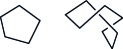
(a) Some trivial knots

(b) Some non-trivial knots

Figure 1. Examples of knots in $\mathbb{R}^{3}$

The input for unknot recognition is typically a knot diagram, i.e., a piecewise-linear projection of the knot $K$ onto the plane in which line segments “cross” over or under one another, as seen in Figure 1. The input size is typically measured by the number of crossings $c$. This is a reasonable measure, since any $c$-crossing knot diagram—regardless of how many line segments it uses—can be deformed into a new diagram of the same topological knot with just $O(c)$ line segments in total.

Only little is known about the computational complexity of unknot recognition. The problem is known to lie in NP [26], and also in co-NP if the generalised Riemann hypothesis holds [35]. Haken’s original algorithm from the 1960s [24] has been improved upon by many authors, but the best derivatives still have worst-case exponential time. There are alternative algorithms, such as Dynnikov’s grid simplification method [21], but these are likewise exponential time or worse. Nevertheless, the former results give us reason to believe that unknot recognition might not be NP-complete, and nowadays there is increasing discussion as to whether a polynomial time algorithm could indeed exist [19, 25].

For inputs that are trivial (i.e., topologically equivalent to the unknot), solving unknot recognition appears to be easy in practice. There are widely-available simplification tools that attempt to “reduce” the input to a smaller representation of the same topological knot in polynomial time [5, 14], and if they can reduce the input all the way down to a circle with no crossings then the problem is solved. Experimentation suggests that it is extremely difficult to find “pathological” representations of the unknot that do not simplify in this way [5, 12].

For input knots that are non-trivial (i.e., not equivalent to the unknot), the situation is more difficult. Here our simplification tools cannot help: they might reduce the input somewhat, but we still need to prove that the resulting knot cannot be completely untangled. There are many computable knot invariants that can assist with this task [2, 37], but all known invariants either come with exponential time algorithms or might lead to inconclusive results (or both).

In this sense, obtaining a “no” answer—that is, proving a knot to be non-trivial—is the more difficult task for unknot recognition. Our new algorithm is fast even in this more difficult case: when run over the KnotInfo database of all $2977$ prime knots with $\leq 12$ crossings [17], it proves each of them to be non-trivial by solving a linear number of linear programming problems. Combined with the aforementioned simplification tools and established polynomial-time algorithms for linear programming [23, 33], this yields the first algorithm for unknot recognition that guarantees a conclusive result and in practice exhibits polynomial-time behaviour.

We note that, although our input knots all have $\leq 12$ crossings, the underlying problems are significantly larger than this figure suggests—our algorithm works in vector spaces of dimension up to $350$ for these inputs. As seen in section 4, both the polynomial profile of our algorithm and the exponential profile of the prior state-of-the-art algorithms (against which we compare it) are unambiguously clear over this data set.

The algorithm is structured as follows. Given a $c$-crossing diagram of the input knot $K$, we construct a corresponding 3-dimensional triangulation $\mathcal{T}$ with $n\in O(c)$ tetrahedra. We then search this triangulation for a certificate of unknottedness, using Haken’s framework of normal surface theory [24]. The search criteria are deliberately weak, which allows us to perform the search using a branch-and-bound method (based on integer and linear programming). The trade-off is that we might find a “false certificate”, which does not certify unknottedness; however, in this case we use our false certificate to shrink the triangulation to fewer tetrahedra, a process which must terminate after at most $n$ iterations.

The bottleneck in this algorithm is the branch-and-bound phase, which in the worst case must traverse a search tree of size $O(3^{n}\cdot n)$. However, the experimental performance is far better: for every one of our input knots, the linear programming relaxations in the branch-and-bound scheme cause the search tree to collapse to $\sim 8n$ nodes, yielding a polynomial-time search overall. This is reminiscent of the simplex method for linear programming, whose worst-case exponential time does not prevent it from being the tool of choice in many practical applications.

We emphasise that this polynomial time behaviour is measured purely by experiment. We do not prove average-case, smoothed or generic complexity results; though highly desirable, such results are scarce in the study of 3-dimensional triangulations. We discuss the reasons for this scarcity in Section 6.

Traditional algorithms based on normal surfaces do not use optimisation; instead they perform an expensive enumeration of extreme rays of a polyhedral cone (see [11, 16] for the computational details). Our use of optimisation follows early ideas of Casson and Jaco et al. [29]: essentially we minimise the genus of a surface in $\mathbb{R}^{3}$ that the knot bounds, which is zero if and only if the knot is trivial. The layout of our branch-and-bound search tree is inspired by earlier work of the present authors on normal surface enumeration algorithms [16].

Optimisation approaches to unknot recognition and related problems have been attempted before, but none have exhibited polynomial-time behaviour to date. The key difficulty is that we must optimise a linear objective function (measuring genus) over a non-convex domain (which encodes potential surfaces). In previous attempts:

• Casson and Jaco et al. split the domain into an exponential number of convex pieces and perform linear programming over each [29]. This gives a useful upper bound on the running time of $O(3^{n}\times\mathrm{poly}(n))$. However, the resulting algorithm is unsuitable because for non-trivial input knots the running time also has a lower bound of $\Omega(3^{n}\times\mathrm{poly}(n))$ [12].

• In prior work, the present authors express this optimisation as an integer program using precise search criteria that guarantee to find a true certificate if one exists (i.e., the criteria are not weakened as described earlier) [15]. The resulting integer programs are extremely difficult to solve in exact arithmetic: they yield useful bounds for invariants such as knot genus and crosscap number, but are unsuitable for decision problems such as unknot recognition.

Beyond unknot recognition, we also adapt our new algorithm to the related topological problems of 3-sphere recognition and prime decomposition of 3-manifolds; see Section 5 for details.

2. Preliminaries

Normal surface theory is a powerful algorithmic toolkit in low-dimensional topology: it sits at the heart of Haken’s original unknot recognition algorithm [24] and provides the framework for the algorithms in this paper. Here we give a very brief overview of knots, triangulations and normal surfaces. For more details on the role this theory plays in unknot recognition and related topological problems, we refer the reader to the excellent summary by Hass et al. [26].

We consider a knot to be a piecewise linear simple closed curve embedded in $\mathbb{R}^{3}$, formed from a finite number of line segments. Two knots $K,K^{\prime}$ are considered equivalent if one can be continuously deformed into the other without introducing self-intersections. Any knot equivalent to a simple planar polygon is said to be trivial, or the unknot; all other knots are said to be non-trivial. Again, see Figure 1 for examples.

A knot diagram is a projection of a knot into the plane with only finitely many multiple points, each of which is a double point at which two “strands” of the knot cross transversely, one “passing over” the other. These double points are called crossings: the four knot diagrams in Figure 1 have 0, 2, 3 and 4 crossings respectively. Alternatively, knot diagrams can be described as annotated 4-valent planar multigraphs; see [26] for the details. A knot diagram with $c$ crossings can (up to knot equivalence) be described in $O(c\log c)$ space (see [28] for some examples of encoding schemes), and in this paper we treat knot diagrams as the usual means by which knots are presented as input.

By adding a point at infinity, we can extend the ambient space from $\mathbb{R}^{3}$ to the topological 3-sphere $S^{3}\equiv\mathbb{R}^{3}\cup\{\infty\}$. For any knot $K$, we can then remove an open regular neighbourhood of $K$ from $S^{3}$ (essentially “drilling out” the knot from $S^{3}$); this yields a 3-manifold with torus boundary called the knot complement $\overline{K}$. Given a knot diagram with $c$ crossings, Hass et al. show how to construct a triangulation of $\overline{K}$ with $O(c)$ tetrahedra in $O(c\log c)$ time [26, Lemma 7.2].

Although the Hass et al. construction produces a simplicial complex, computational topologists often work with generalised triangulations, which are more flexible and often significantly smaller. A generalised triangulation begins with $n$ abstract tetrahedra, and affinely identifies (or “glues”) some or all of their $4n$ triangular faces in pairs. Two different faces of the same tetrahedron may be glued together; moreover, as a consequence of the face gluings we may find that multiple edges of the same tetrahedron become identified together, and likewise with vertices. Unless otherwise specified, all triangulations in this paper are generalised triangulations.

Of particular importance are one-vertex triangulations, in which all $4n$ tetrahedron vertices become identified as a single point. Essentially, these are the 3-dimensional analogues of well-known constructions in two dimensions, such as the two-triangle torus and the two-triangle Klein bottle shown in Figure 2 (the different arrowheads indicate how edges are glued together)—both of these 2-dimensional examples are one-vertex triangulations also.

(a) A torus

(b) A Klein bottle

Figure 2. Triangulated surfaces in two dimensions

If a triangulation $\mathcal{T}$ represents some underlying 3-manifold $\mathcal{M}$, then those tetrahedron faces of $\mathcal{T}$ that are not glued to a partner together form a triangulated surface (possibly empty, possibly disconnected) which we call the boundary of $\mathcal{T}$, denoted by $\partial\mathcal{T}$; topologically this represents the 3-manifold boundary $\partial\mathcal{M}$.

A normal surface in $\mathcal{T}$ is a surface $S$ that is properly embedded (i.e., embedded so that $\partial S=S\cap\partial\mathcal{T}$), and which meets each tetrahedron of $\mathcal{T}$ in a (possibly empty) collection of curvilinear triangles and quadrilaterals, as illustrated in Figure 3(a). In each tetrahedron these triangles and quadrilaterals are classified into seven types according to which edges of the tetrahedron they meet, as illustrated in Figure 3(b): four triangle types (each “truncating” one of the four vertices), and three quadrilateral types (each separating the four vertices into two pairs).

(a) The surface $S$ meeting a single tetrahedron

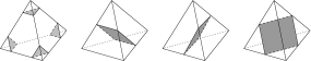
(b) The seven normal disc types

Figure 3. Normal triangles and quadrilaterals

Any normal surface $S$ in an $n$-tetrahedron triangulation $\mathcal{T}$ can be described by a vector of $7n$ non-negative integers that counts the number of triangles and quadrilaterals of each type in each tetrahedron; we denote this by $\mathbf{v}(S)\in\mathbb{Z}^{7n}$. The individual coordinates of $\mathbf{v}(S)$ that count triangles and quadrilaterals are referred to as triangle and quadrilateral coordinates respectively. This vector uniquely identifies the surface (up to a certain class of isotopy). More generally, a result of Haken [24] shows that an integer vector $\mathbf{x}\in\mathbb{R}^{7n}$ represents a normal surface if and only if:

1. $\mathbf{x}\geq 0$;

2. $A\mathbf{x}=0$, where $A$ is a matrix of up to $6n$ linear matching equations derived from the specific triangulation $\mathcal{T}$;

3. $\mathbf{x}$ satisfies the quadrilateral constraints, a collection of $n$ combinatorial constraints (one per tetrahedron) that require, for each tetrahedron, at most one of the three corresponding quadrilateral coordinates to be non-zero.

In essence, the matching equations ensure that normal triangles and quadrilaterals can be glued together across adjacent tetrahedra, and the quadrilateral constraints ensure that quadrilaterals within the same tetrahedron can avoid intersecting. Any vector $\mathbf{x}\in\mathbb{R}^{7n}$ (real or integer) that satisfies all three of these conditions is called admissible.

The Euler characteristic of a surface, denoted $\chi$, is a topological invariant that essentially encodes the genus of the surface. In particular, an orientable surface of genus $g$ with $b$ boundary curves has Euler characteristic $\chi=2-2g-b$, and a non-orientable surface of genus $g$ with $b$ boundary curves has Euler characteristic $\chi=2-g-b$. Given any polygonal decomposition of a surface, its Euler characteristic can be computed as $\chi=V-E+F$, where $V$, $E$ and $F$ count vertices, edges and 2-faces respectively.

For normal surfaces within a fixed $n$-tetrahedron triangulation $\mathcal{T}$, their Euler characteristics can be expressed using a homogeneous linear function on normal coordinates. That is, there is a homogeneous linear function $\chi\colon\thinspace\mathbb{R}^{7n}\to\mathbb{R}$ such that, if $S$ is any normal surface in $\mathcal{T}$, then $\chi(\mathbf{v}(S))$ is the Euler characteristic of $S$. In fact there are many choices for such a function; see [15, 32] as well as the proof of Lemma 10 in this paper for various formulations.

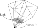
Figure 4. Building a vertex link from triangles

Let $V$ be a vertex of some triangulation $\mathcal{T}$. Then the link of $V$ is the frontier of a small regular neighbourhood of $V$. In a 3-manifold triangulation, each vertex link is either a disc (for a boundary vertex $V\in\partial\mathcal{T}$) or a sphere (for an internal vertex $V\notin\partial\mathcal{T}$). The link can be presented as a normal surface built from triangles only (see Figure 4), and if $\mathcal{T}$ is a one-vertex triangulation then this normal surface contains precisely one triangle of each type.

Figure 5. A disc bounded by a trivial knot

Haken’s original unknot recognition algorithm is based on the observation that any trivial knot must bound an embedded disc in $\mathbb{R}^{3}$ (see Figure 5). In the knot complement $\overline{K}$, this corresponds to a properly embedded disc in $\overline{K}$ that meets the boundary torus $\partial\overline{K}$ in a non-trivial curve (i.e., a curve that does not bound a disc in $\partial\overline{K}$). Moreover, we have:

Theorem 1 (Haken).

Let $K$ be a knot and let $\mathcal{T}$ be a triangulation of the complement $\overline{K}$. Then $K$ is trivial if and only if $\mathcal{T}$ contains a normal disc whose boundary is a non-trivial curve in $\partial\mathcal{T}$.

3. The algorithm

In this paper we describe the new algorithm at a fairly high level. For details of the underlying data structures, we refer the reader to the thoroughly documented source code for the software package Regina [14], in which this algorithm is implemented.

At the highest level, the new algorithm operates as follows.

Algorithm 2 (Unknot recognition).

To test if an input knot $K$ is trivial, given a knot diagram of $K$:

1. Build a triangulation of the knot complement $\overline{K}$.

2. Make this into a one-vertex triangulation $\mathcal{T}$ of $\overline{K}$ without increasing the number of tetrahedra. Let the number of tetrahedra in $\mathcal{T}$ be $n$.

3. Search for a connected normal surface $S$ in $\mathcal{T}$ which is not the vertex link and has positive Euler characteristic.

   • If no such $S$ exists, then the knot $K$ is non-trivial.

   • If $S$ is a disc whose boundary is a non-trivial curve in $\partial\mathcal{T}$, then the knot $K$ is trivial.

   • Otherwise we modify $\mathcal{T}$ by crushing the surface $S$ to obtain a new triangulation $\mathcal{T}^{\prime}$ of $\overline{K}$ with fewer than $n$ tetrahedra, and return to step 2 using this new triangulation $\mathcal{T}^{\prime}$ instead.

To build the initial triangulation of $\overline{K}$ in step 1, we use the method of Hass et al. [26, Lemma 7.2] as noted earlier in the preliminaries section. For the subsequent steps, we give details in separate sections below:

• To make a one-vertex triangulation in step 2, we combine the Jaco-Rubinstein crushing procedure (described in Section 3.1) with a combinatorial expansion procedure (described in Section 3.2).

• To find the surface $S$ in step 3, we use techniques from integer and linear programming (described in Section 3.3). This search is the main bottleneck—and hence the most critical component—of the algorithm.

• To crush $S$ in step 3, we once more use the Jaco-Rubinstein procedure (again see Section 3.1).

After presenting these details, in Section 3.4 we prove the algorithm correct and analyse its time complexity. In particular, we show that the search for $S$ in step 3 is the only potential source of exponential time. That is, if the search for $S$ exhibits polynomial time in practice (as we quantify experimentally in Section 4), then this translates to polynomial-time behaviour in practice for the algorithm as a whole.

3.1. The Jaco-Rubinstein crushing procedure

Steps 2 and 3 of the algorithm above make use of the crushing procedure of Jaco and Rubinstein, which modifies a triangulation by “destructively” crushing a normal surface within it. Here we outline this procedure, and then prove in Lemma 5 that (i) in our setting it yields a smaller triangulation of the knot complement $\overline{K}$, and (ii) this smaller triangulation can be obtained in linear time.

Our outline of the crushing procedure is necessarily brief. See the original Jaco-Rubinstein paper [31] for the full details, or [13] for a simplified approach.

Mathematically, the crushing procedure operates as follows. Given a normal surface $S$ within a triangulation $\mathcal{T}$, we first cut $\mathcal{T}$ open along $S$ and then collapse all of the triangles and quadrilaterals of $S$ (which now appear twice each on the boundary) to points, as shown in Figure 6(a). This results in a new cell complex that is typically not a triangulation, but instead is built from a combination of tetrahedra, footballs and/or pillows as illustrated in Figure 6(b). We then flatten each football to an edge and each pillow to a triangular face, as shown in Figure 6(c), resulting in a new triangulation $\mathcal{T}^{c}$ that is the final result of the crushing procedure. In general this final triangulation $\mathcal{T}^{c}$ might be disconnected, might represent a different 3-manifold from $\mathcal{T}$, or might not even represent a 3-manifold at all. We now make two important observations, both due to Jaco and Rubinstein [31]:

(a) Cutting along and then collapsing a surface

(b) Intermediate pieces

(c) Flattening footballs and pillows

Figure 6. The Jaco-Rubinstein crushing procedure

Observation 3.

The tetrahedra in $\mathcal{T}^{c}$ (i.e., those that “survive” the crushing process) correspond precisely to those tetrahedra in $\mathcal{T}$ that do not contain any quadrilaterals of $S$. In particular, unless $S$ is a collection of vertex links, the number of tetrahedra in $\mathcal{T}^{c}$ will be strictly smaller than in $\mathcal{T}$.

Observation 4.

If $S$ is a normal sphere or disc and $\mathcal{T}$ triangulates an orientable 3-manifold $\mathcal{M}$ (with or without boundary), then the result $\mathcal{T}^{c}$ triangulates some new 3-manifold $\mathcal{M}^{c}$ (possibly disconnected or empty) that is obtained from $\mathcal{M}$ by zero or more of the following operations:

1. cutting $\mathcal{M}$ open along spheres and filling the resulting boundary spheres with 3-balls;

2. cutting $\mathcal{M}$ open along properly embedded discs;

3. capping boundary spheres of $\mathcal{M}$ with 3-balls;

4. deleting entire connected components that are any of the 3-ball, the 3-sphere, projective space $\mathbb{R}P^{3}$, the lens space $L_{3,1}$ or the product space $S^{2}\times S^{1}$.

See [13, Theorem 2] for a simplified treatment and proof of Observation 4.

Our result below uses both of these observations to show that crushing does what we need in our setting. Moreover, it shows through amortised complexity arguments that, with the right implementation, crushing can be carried out in linear time.

Lemma 5.

Given a triangulation $\mathcal{T}$ of a knot complement $\overline{K}$ with $n>1$ tetrahedra and a connected normal surface $S$ in $\mathcal{T}$ which is not a vertex link and which has positive Euler characteristic, we can crush $S$ using the Jaco-Rubinstein procedure and convert the result into a new triangulation $\mathcal{T}^{\prime}$ of $\overline{K}$ with strictly fewer than $n$ tetrahedra, all in $O(n)$ time.

Proof.

The only connected surfaces with positive Euler characteristic are the sphere, the disc, and the projective plane. Since $\mathcal{T}$ triangulates a knot complement in $S^{3}$ and $S^{3}$ does not contain an embedded projective plane, we conclude that our surface $S$ is either a sphere or a disc.

We first show how to build a smaller triangulation $\mathcal{T}^{\prime}$ of $\overline{K}$. We begin by crushing $S$ in $\mathcal{T}$ to obtain an intermediate triangulation $\mathcal{T}^{c}$. Since $\overline{K}$ is a knot complement, the list of possible topological changes from Observation 4 becomes much simpler:

1. Any embedded sphere in a knot complement bounds a ball, and so the first operation (cutting along spheres and filling the boundaries with balls) is equivalent to adding new (disconnected) 3-sphere components.

2. The result of cutting along a properly embedded disc $D$ depends on the boundary of this disc. If the boundary of $D$ is trivial on the torus $\partial\overline{K}$, then since $\overline{K}$ is a knot complement it must be true that $D$ and some portion of $\partial\overline{K}$ together bound a 3-ball, and cutting along $D$ simply adds a new 3-ball component. If the boundary of $D$ is non-trivial on $\partial\overline{K}$ then $K$ must be a trivial knot, and cutting along $D$ converts the entire manifold $\overline{K}$ into the 3-ball.

3. The only boundary spheres that might occur will be the boundaries of new 3-ball components created in the previous step. Capping these spheres with 3-balls has the effect of converting these new 3-ball components into new 3-sphere components instead.

4. If we begin with a knot complement, none of the operations above can ever produce the manifolds $\mathbb{R}P^{3}$, $L_{3,1}$ or $S^{2}\times S^{1}$. Therefore the only connected components that we could ever delete are 3-balls and 3-spheres.

In other words, the topological changes introduced in the intermediate triangulation $\mathcal{T}^{c}$ are limited to possibly replacing $\overline{K}$ with a 3-ball (but only if the knot $K$ is trivial), and adding or removing 3-ball and/or 3-sphere components.

It is clear now how to obtain the new triangulation $\mathcal{T}^{\prime}$ of $\overline{K}$. If any connected component of the intermediate triangulation $\mathcal{T}^{c}$ has torus boundary then we can take this component as the new triangulation $\mathcal{T}^{\prime}$. Otherwise we know that $K$ must be the trivial knot, and we can take $\mathcal{T}^{\prime}$ to be the standard one-tetrahedron triangulation of the solid torus [31] (though we could of course just terminate the unknot recognition algorithm immediately). Either way, $\mathcal{T}^{\prime}$ triangulates the same knot complement $\overline{K}$.

Because $S$ is not the vertex link, it contains at least one quadrilateral and so crushing will strictly reduce the number of tetrahedra (recall Observation 3 above). It is clear then that after extracting the component with torus boundary (or building a new one-tetrahedron solid torus), the number of tetrahedra in $\mathcal{T}^{\prime}$ will be strictly less than $n$.

We now show how to obtain this smaller triangulation $\mathcal{T}^{\prime}$ in $O(n)$ time. There are two procedures that we must analyse: (i) the Jaco-Rubinstein crushing procedure (converting $\mathcal{T}\to\mathcal{T}^{c}$), and (ii) extracting the connected component with torus boundary if one exists (converting $\mathcal{T}^{c}\to\mathcal{T}^{\prime}$).

• The crushing procedure (converting $\mathcal{T}\to\mathcal{T}^{c}$):

  It is simple to identify which tetrahedra of $\mathcal{T}$ survive the crushing procedure (those whose corresponding quadrilateral coordinates in $S$ are all zero, as in Observation 3)—the main challenge is to identify in $O(n)$ time how the faces of these surviving tetrahedra are to be glued together.

  Let $\phi$ be some face of a surviving tetrahedron $\Delta$. To identify the new partner face for $\phi$, we trace a path through adjacent tetrahedra in the original triangulation $\mathcal{T}$ as follows. Whenever we enter a tetrahedron that contains quadrilaterals of $S$, we cross to the face on the opposite side of these quadrilaterals (as depicted in Figure 7(a)) and continue through to the next adjacent tetrahedron. If we ever reach a tetrahedron with no quadrilaterals of $S$, then the resulting face $\phi^{\prime}$ is the partner to which $\phi$ is glued. If instead we reach the boundary $\partial\mathcal{T}$, then $\phi$ becomes a boundary face of the new triangulation. See Figure 7(b) for a full illustration.

  

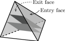
  (a) Crossing to the opposite side of the quadrilaterals

  

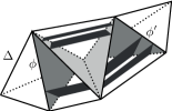
  (b) Moving from $\phi$ to the partner face $\phi^{\prime}$

  Figure 7. Identifying the face gluings after crushing

  To see why following paths in this way correctly identifies the face gluings, we must study the way in which pillows (formed on either side of the quadrilaterals in a tetrahedron) flatten to triangles, as seen earlier in Figure 6(c). Jaco and Rubinstein explain this in their original paper [31], and we do not reiterate the details here. It is important to note that such a path cannot cycle (since the starting tetrahedron $\Delta$ does not contain quadrilaterals), and so we must eventually reach one of the two conclusions described above.

  Regarding time complexity: although any individual path may be long, we note that each tetrahedron of $\mathcal{T}$ can feature at most twice amongst all the paths (once for each of the two directions in which we might cross over the quadrilaterals). Therefore the total length of all such paths is $O(n)$. Each step in such a path takes $O(1)$ time to compute (since all we need to know is which, if any, of the three quadrilateral coordinates is non-zero in the next tetrahedron), and so the gluings in the crushed triangulation $\mathcal{T}^{c}$ can all be computed in total $O(n)$ time.

• Extracting the component with torus boundary (converting $\mathcal{T}^{c}\to\mathcal{T}^{\prime}$):

  Since each tetrahedron is adjacent to at most four neighbours, we can identify connected components of $\mathcal{T}^{c}$ in $O(n)$ time by following a depth-first search through adjacent tetrahedra for each component. This takes $O(t)$ time for each $t$-tetrahedron component, summing to $O(n)$ time overall.

  For each connected component, we “build the skeleton”; that is, group the $4t$ vertices, $6t$ edges and $4t$ faces of the $t$ individual tetrahedra into equivalence classes that indicate how these are identified (or “glued together”) in the triangulation. As before, we do this by following a depth-first search through adjacent tetrahedra for each equivalence class. Each search requires time proportional to the size of the equivalence class, summing to $O(t)$ time for each component and $O(n)$ time overall.

  For components with non-empty boundary, we can test for torus boundary by counting equivalence classes of vertices, edges and faces, and computing the Euler characteristic $\chi=\mathrm{vertices}-\mathrm{edges}+\mathrm{faces}-\mathrm{tetrahedra}$. This is enough to distinguish between components with torus boundary ($\chi=0$) versus sphere boundary ($\chi=1$), which from earlier are the only possible scenarios after crushing. Once again this sums to $O(n)$ time overall. ∎

3.2. Building a one-vertex triangulation

In step 2 of Algorithm 2, we convert our existing triangulation of $\overline{K}$ into a one-vertex triangulation of $\overline{K}$. There are well-known algorithms for producing one-vertex triangulations of a 3-manifold [31, 38], though they have not been studied from a complexity viewpoint. We give a method that combines Jaco-Rubinstein crushing with a tightly-controlled subcomplex expansion technique, and show that it runs in small polynomial time.

Before we formally state and prove this result, we introduce some terminology.

Definition.

Let $\mathcal{E}$ be a subcomplex of a triangulation $\mathcal{T}$; that is, a union of vertices, edges, triangles and/or tetrahedra of $\mathcal{T}$. Then by the neighbourhood of $\mathcal{E}$, denoted by $\mathop{nbd}(\mathcal{E})$, we mean the closure of a small regular neighbourhood of $\mathcal{E}$. By the link of $\mathcal{E}$, denoted by $\mathop{lk}(\mathcal{E})$, we refer to the frontier of this neighbourhood.

(a) A subcomplex $\mathcal{E}$

(b) The neighbourhood $\mathop{nbd}(\mathcal{E})$

(c) The link $\mathop{lk}(\mathcal{E})$

Figure 8. Neighbourhood and link in a 2-dimensional triangulation

Figure 8 illustrates both concepts in the 2-dimensional setting, using a triangulation of the disc. In our 3-dimensional setting, $\mathop{nbd}(\mathcal{E})$ is always a 3-manifold with boundary, and $\mathop{lk}(\mathcal{E})$ (which generalises the earlier concept of a vertex link) is always a properly embedded surface in $\mathcal{T}$.

Lemma 6.

Given an $n$-tetrahedron triangulation $\mathcal{T}$ of a knot complement $\overline{K}$, we can construct a one-vertex triangulation $\mathcal{T}^{\prime}$ of $\overline{K}$ with at most $n$ tetrahedra in $O(n^{3})$ time.

Proof.

First we count the number of vertices of $\mathcal{T}$. We can do this in $O(n)$ time by partitioning the $4n$ individual tetrahedron vertices into equivalence classes that indicate how they are identified in the overall triangulation, using a depth-first search through the gluings between adjacent tetrahedra.

If $\mathcal{T}$ has only one vertex, then we are finished. Therefore we assume from here on that $\mathcal{T}$ has more than one vertex. It follows immediately that we have $n\geq 2$ tetrahedra, since by a simple enumeration of all one-tetrahedron triangulations, the only one-tetrahedron knot complement is the standard one-tetrahedron, one-vertex triangulation of the solid torus [31].

Our next task is to locate an edge $e$ that joins two distinct vertices of $\mathcal{T}$. If $\mathcal{T}$ contains more than one vertex on the boundary then we choose $e$ to lie entirely in $\partial\mathcal{T}$ (as opposed to cutting through the interior of $\mathcal{T}$); otherwise we choose $e$ to join the single boundary vertex with some internal vertex (as opposed to joining two internal vertices). We can find such an edge in $O(n)$ time simply by iterating through all $6n$ individual tetrahedron edges, and observing how their endpoints sit within the partition of vertices that we made before.

Our plan is to convert this edge $e$ into a normal disc that is not a vertex link, and to do this in $O(n^{2})$ time. Given such a normal disc, Lemma 5 shows that we can crush it in $O(n)$ time to obtain a new triangulation of $\overline{K}$ with strictly fewer tetrahedra. We repeat this process until we arrive at a one-vertex triangulation; since the number of tetrahedra decreases at every stage, the process must terminate after at most $n$ iterations, giving a running time of $O(n^{3})$ overall.

The remainder of this proof shows how, given our edge $e$, we can build a non-vertex-linking normal disc in $O(n^{2})$ time.

From our choice of $e$, the link $\mathop{lk}(e)$ is already a disc; however, it might not be normal. For instance, if $e$ appears twice around some triangle of $\mathcal{T}$, then the link of $e$ will meet this triangle in a “bent” arc (shown in Figure 9), which a normal surface cannot contain.

Figure 9. A non-normal edge linking surface

Our strategy then is to expand $e$ to a subcomplex $\mathcal{E}$ of $\mathcal{T}$ whose link $\mathop{lk}(\mathcal{E})$ is a normal surface, and to show that some component of this link is the disc that we seek. To do this, we initialise $\mathcal{E}$ to the single edge $e$ and repeat the following expansion steps for as long as possible:

• If any triangle has either two or all three of its edges in $\mathcal{E}$, we expand $\mathcal{E}$ to include the entire triangle (as illustrated in Figure 10);

• If any tetrahedron has all four of its triangular faces in $\mathcal{E}$, we expand $\mathcal{E}$ to include the entire tetrahedron.

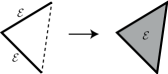
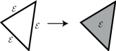
Figure 10. Expanding the subcomplex $\mathcal{E}$

We now present a series of claims that together show that some component of $\mathop{lk}(\mathcal{E})$ is a non-vertex-linking normal disc. After this, we conclude the proof by showing how this disc is constructed in $O(n^{2})$ time.

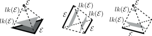
Figure 11. Building the link $\mathop{lk}(\mathcal{E})$ as a normal surface

Claim A: Once the expansion is finished, the link $\mathop{lk}(\mathcal{E})$ is normal.

To show this, we explicitly construct $\mathop{lk}(\mathcal{E})$ by inserting the following triangles and quadrilaterals into each tetrahedron $\Delta$ of $\mathcal{T}$ (see Figure 11 for illustrations):

• If $\mathcal{E}$ contains the entire tetrahedron $\Delta$, then we do not place any triangles or quadrilaterals in $\Delta$.

• Otherwise, $\mathcal{E}$ contains at most one triangular face of $\Delta$ (since two or more faces would cause the expansion process to consume $\Delta$ completely). If $\mathcal{E}$ does contain a face of $\Delta$, then we place a normal triangle beside this face.

• If $\mathcal{E}$ does not contain any faces of $\Delta$, it might still contain either one edge of $\Delta$, or two opposite edges of $\Delta$ (any more would again cause further expansion). If $\mathcal{E}$ contains such edge(s), then we place a normal quadrilateral beside each edge.

• If $\mathcal{E}$ contains any additional vertices of $\Delta$ that are not yet accounted for, we place a triangle next to each such vertex.

When connected together, these triangles and quadrilaterals form the link $\mathop{lk}(\mathcal{E})$, thereby establishing claim A.

Claim B: The neighbourhood $\mathop{nbd}(\mathcal{E})$ is a 3-ball, possibly with punctures, and $\mathop{nbd}(\mathcal{E})$ meets the boundary $\partial\mathcal{T}$ in a non-empty connected region.

We prove this by induction, showing that claim B holds true at each stage of the expansion process.

• At the beginning of the expansion process we have $\mathcal{E}=e$. Here our claim is true because we chose $e$ to join two distinct vertices, and because we chose $e$ to meet $\partial\mathcal{T}$ in either (i) just one endpoint, or (ii) the entire edge. Either way, $\mathop{nbd}(e)$ is just a 3-ball that meets $\partial\mathcal{T}$ in a disc.

• Suppose some triangle of $\mathcal{T}$ has two of its edges in $\mathcal{E}$. The resulting expansion step “grows” both $\mathcal{E}$ and $\mathop{nbd}(\mathcal{E})$ to include the entire triangle (see Figure 12(a)). This does not change the topology of $\mathop{nbd}(\mathcal{E})$, which remains a 3-ball possibly with punctures.

  If the third edge of the triangle is internal to $\mathcal{T}$ then the intersection $\mathop{nbd}(\mathcal{E})\cap\partial\mathcal{T}$ does not change. If the third edge lies in the boundary of $\mathcal{T}$ then the intersection $\mathop{nbd}(\mathcal{E})\cap\partial\mathcal{T}$ expands but remains connected (we effectively attach a strip surrounding this third edge).

  

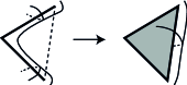
  (a) Growing $\mathcal{E}$ across a triangle

  

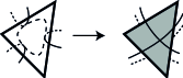
  (b) Expanding $\mathcal{E}$ into a triangle

  Figure 12. How expansion affects the neighbourhood $\mathop{nbd}(\mathcal{E})$

• Suppose some triangle of $\mathcal{T}$ has all three of its edges in $\mathcal{E}$. Here the expansion attaches a thickened disc to $\mathop{nbd}(\mathcal{E})$ (see Figure 12(b)), which converts $\mathop{nbd}(\mathcal{E})$ from a 3-ball with $k$ punctures to a 3-ball with $k+1$ punctures.

  As before, if the triangle is internal to $\mathcal{T}$ then the intersection $\mathop{nbd}(\mathcal{E})\cap\partial\mathcal{T}$ does not change, and if the triangle lies in the boundary of $\mathcal{T}$ then the intersection expands but remains connected.

• Finally, if a tetrahedron has all four of its faces in $\mathcal{E}$, the resulting expansion simply “closes off” one of the punctures in $\mathop{nbd}(\mathcal{E})$ by filling it with a ball.

Inducting over the step-by-step construction of $\mathcal{E}$ now establishes claim B.

Claim C: Some component of the link $\mathop{lk}(\mathcal{E})$ is a disc that is not a vertex link.

Let $I=\mathop{nbd}(\mathcal{E})\cap\partial\mathcal{T}$. By claim B, $\mathop{nbd}(\mathcal{E})$ is bounded by spheres, and so $I$ (which is a non-empty, connected subset of this boundary) must be a sphere with zero or more punctures. Because $\partial\mathcal{T}$ is a torus, $I\neq\partial\mathcal{T}$; therefore the surface $I$ has boundary, and must be a sphere with at least one puncture.

Let $S$ be the particular sphere bounding $\mathop{nbd}(\mathcal{E})$ that contains $I$ as a subset. When combined, the link $\mathop{lk}(\mathcal{E})$ and $I$ together form the entire boundary of $\mathop{nbd}(\mathcal{E})$; therefore $\mathop{lk}(\mathcal{E})$ is the disjoint union of (i) zero or more spheres (excluding $S$), and (ii) one or more discs (which “plug the punctures” left by $I$ on the sphere $S$). If all of these latter discs are vertex links, then all of the punctures in $I$ must also be filled with discs on $\partial\mathcal{T}$ (see Figure 13); however, this would make $\partial\mathcal{T}$ a sphere (not a torus), and so at least one of these discs must not be a vertex link. This establishes claim C.

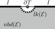
Figure 13. A vertex linking component of $\mathop{lk}(\mathcal{E})$

Conclusion: By claims A and C, some component of $\mathop{lk}(\mathcal{E})$ is the non-vertex-linking normal disc that we seek. All that remains is to show that we can construct this disc in $O(n^{2})$ time.

To build the subcomplex $\mathcal{E}$ from the original edge $e$ takes $O(n^{2})$ time: each expansion step can be tested and performed in $O(n)$ time, and since $\mathcal{T}$ contains $O(n)$ edges, triangles and tetrahedra there are $O(n)$ expansion steps in total.

Building the normal surface $\mathop{lk}(\mathcal{E})$ now takes $O(n)$ time, since (from Claim A) we simply insert $O(1)$ triangles and/or quadrilaterals in each tetrahedron. Moreover, this normal surface contains $O(n)$ triangles and quadrilaterals in total, and so in $O(n)$ time we can extract the connected components of $\mathop{lk}(\mathcal{E})$, compute their Euler characteristics, and identify one such component that is a disc but not a vertex link. This concludes the proof of Lemma 6. ∎

3.3. Searching for positive Euler characteristic

We now give the details for step 3 of Algorithm 2, in which we search through our triangulation for a connected normal surface which is not the vertex link and has positive Euler characteristic. This search sits at the heart of the algorithm, and is its major bottleneck.

Assumptions.

Throughout this section, $\mathcal{T}$ is a one-vertex, $n$-tetrahedron triangulation of a knot complement $\overline{K}$.

In principle, our search treats the Euler characteristic $\chi\colon\thinspace\mathbb{R}^{7n}\to\mathbb{R}$ as a linear objective function, and maximises $\chi$ over the space of admissible points in $\mathbb{R}^{7n}$ using branch-and-bound techniques. If the surface we are seeking exists then the maximum $\chi$ will be unbounded (because the matching equations, quadrilateral constraints and $\chi$ are all homogeneous, and so admissible points with $\chi>0$ can be scaled arbitrarily). If the surface we are seeking does not exist then the maximum $\chi$ will be zero (because $\mathbf{0}\in\mathbb{R}^{7n}$ is always admissible). In practice, since we only need to distinguish between a zero or positive maximum, we formulate our search purely in terms of branching and feasibility tests.

We begin this section with Lemmata 7 and 8, which set up constraints for our search: Lemma 7 shows we can ensure our surface is connected by setting as many coordinates as possible to zero, and Lemma 8 shows we can ensure our surface is not the vertex link by setting at least one triangle coordinate to zero. We follow with a description of Algorithm 9, which lays out the structure of the search, and then we discuss the details of the branching scheme, prove correctness, and analyse the running time.

Recall from the preliminaries section that, if $S$ is a normal surface in $\mathcal{T}$, then $\mathbf{v}(S)$ denotes the vector representation of $S$ in $\mathbb{R}^{7n}$. Recall also that a point $\mathbf{x}\in\mathbb{R}^{7n}$ is admissible if it satisfies $\mathbf{x}\geq 0$, the matching equations $A\mathbf{x}=0$, and the quadrilateral constraints.

Lemma 7.

Let $S$ be a normal surface in $\mathcal{T}$ with positive Euler characteristic, and suppose there is no normal surface $S^{\prime}$ in $\mathcal{T}$ with positive Euler characteristic with the following properties: (i) whenever the $i$th coordinate of $\mathbf{v}(S)$ is zero then the $i$th coordinate of $\mathbf{v}(S^{\prime})$ is likewise zero; and (ii) there is some $i$ for which the $i$th coordinate of $\mathbf{v}(S)$ is non-zero but the $i$th coordinate of $\mathbf{v}(S^{\prime})$ is zero.

Then the smallest positive rational multiple of $\mathbf{v}(S)$ whose coordinates are all integers represents a connected normal surface with positive Euler characteristic.

Proof.

Let $\mathcal{C}$ denote the polyhedral cone in $\mathbb{R}^{7n}$ defined by $\mathbf{x}\geq 0$ and $A\mathbf{x}=0$. We first show that the vector $\mathbf{v}(S)$ lies on an extreme ray of $\mathcal{C}$ (in the language of normal surface theory, such an $S$ is called a vertex normal surface).

Suppose that $\mathbf{v}(S)$ does not lie on an extreme ray of $\mathcal{C}$. Since $\mathbf{v}(S)$ is admissible we have $\mathbf{v}(S)\in\mathcal{C}$, and so we can express $\mathbf{v}(S)$ as a finite non-negative linear combination $\mathbf{v}(S)=\lambda_{1}\mathbf{e}_{1}+\ldots+\lambda_{k}\mathbf{e}_{k}$, where each $\mathbf{e}_{i}$ lies on a different extreme ray of $\mathcal{C}$, each $\lambda_{i}>0$, and there are $k\geq 2$ terms. Because $\mathcal{C}$ is a rational cone, we can take each $\mathbf{e}_{i}$ to be an integer vector. Since $\mathcal{C}$ lies in the non-negative orthant, it follows that whenever the $i$th coordinate of $\mathbf{v}(S)$ is zero then the $i$th coordinate of each $\mathbf{e}_{i}$ must likewise be zero. In particular, since $\mathbf{v}(S)$ satisfies the quadrilateral constraints, each $\mathbf{e}_{i}$ also satisfies the quadrilateral constraints, and so each $\mathbf{e}_{i}=\mathbf{v}(S_{i})$ for some normal surface $S_{i}$.

Recall that the Euler characteristic $\chi$ is a homogeneous linear function on $\mathbb{R}^{7n}$. Since $\chi(\mathbf{v}(S))>0$, we have $\chi(\mathbf{e}_{p})>0$ for some summand $\mathbf{e}_{p}$; i.e., the corresponding surface $S_{p}$ has positive Euler characteristic. Take any other summand $\mathbf{e}_{q}$ where $q\neq p$. Since the inequalities that define $\mathcal{C}$ are all of the form $x_{i}\geq 0$, the extreme rays of $\mathcal{C}$ are defined by which coordinates are zero and which are non-zero; in particular, there must be some coordinate which is non-zero in $\mathbf{e}_{q}$ but zero in $\mathbf{e}_{p}$. This coordinate is therefore non-zero in $\mathbf{v}(S)$ but zero in $\mathbf{v}(S_{p})$, and so the surface $S_{p}$ satisfies all of the properties of $S^{\prime}$ in the lemma statement, yielding a contradiction.

Therefore $\mathbf{v}(S)$ lies on an extreme ray of $\mathcal{C}$. Let $\mathbf{u}$ be the smallest positive rational multiple of $\mathbf{v}(S)$ with integer coordinates. It is clear that, like $\mathbf{v}(S)$, $\mathbf{u}$ is also admissible with $\chi(\mathbf{u})>0$; that is, $\mathbf{u}$ represents some normal surface $U$ with positive Euler characteristic. All that remains to show is that $U$ is connected.

If $U$ is not connected, we can express it as the disjoint union of non-empty normal surfaces $U=X\cup Y$, whereupon $\mathbf{u}=\mathbf{v}(X)+\mathbf{v}(Y)$. Since $\mathbf{u}$ lies on an extreme ray of $\mathcal{C}$, it must be that both $\mathbf{v}(X)$ and $\mathbf{v}(Y)$ are smaller integer multiples of $\mathbf{u}$, in contradiction with the definition of $\mathbf{u}$. ∎

Lemma 8.

A connected normal surface $S$ in $\mathcal{T}$ is the vertex link if and only if the vector $\mathbf{v}(S)\in\mathbb{R}^{7n}$ has none of its $4n$ triangle coordinates equal to zero.

Proof.

This is an immediate consequence of the fact that $\mathcal{T}$ is one-vertex. The vertex link itself has all triangle coordinates equal to one, and any other surface whose triangle coordinates are all positive must be the disconnected union of the vertex link with one or more other surfaces. ∎

Algorithm 9.

To find a connected normal surface $S$ which is not the vertex link and which has positive Euler characteristic:

1. Search for an admissible point $\mathbf{p}\in\mathbb{R}^{7n}$ for which $\chi(\mathbf{p})\geq 1$, and for which at least one of the $4n$ triangle coordinates is zero. If no such $\mathbf{p}$ exists then the surface $S$ does not exist either.

2. Construct a system $\mathcal{L}$ of linear constraints, initially defined by $\mathbf{x}\geq 0$, $\chi(\mathbf{x})\geq 1$, and the matching equations $A\mathbf{x}=0$. Using the point $\mathbf{p}$ located in the previous step:

   1. For each coordinate $i=1,\ldots,7n$ with $p_{i}=0$, add the additional constraint $x_{i}=0$ to the system $\mathcal{L}$.

   2. Then, for each coordinate $i=1,\ldots,7n$ with $p_{i}\neq 0$, add the constraint $x_{i}=0$ to $\mathcal{L}$ and test whether $\mathcal{L}$ is feasible (i.e., has any solutions). If so, keep the constraint $x_{i}=0$ in $\mathcal{L}$; if not, remove it again.

3. Let $\mathbf{q}$ be a solution to the final system $\mathcal{L}$, and let $\lambda\mathbf{q}$ be the smallest positive rational multiple of $\mathbf{q}$ whose coordinates are all integers. Then $\lambda\mathbf{q}$ is an integer vector in $\mathbb{R}^{7n}$ that represents the desired surface $S$.

In summary: step 1 contains the bulk of the work in locating a solution if one exists, and requires worst-case exponential time. If a solution is found then steps 2 and 3 refine it in polynomial time by setting as many additional coordinates to zero as possible, which ensures that the final normal surface is connected (as in Lemma 7) without violating the quadrilateral constraints.

We analyse this algorithm shortly (see Lemma 10, which proves correctness and bounds the time complexity). First, however, we describe in detail the branching scheme used to search for the point $\mathbf{p}$ in step 1. Specifically, we are searching for a (rational) point $\mathbf{x}\in\mathbb{R}^{7n}$ that satisfies:

1. $\mathbf{x}\geq 0$;

2. the matching equations $A\mathbf{x}=0$;

3. the quadrilateral constraints;

4. $\chi(\mathbf{x})\geq 1$; and

5. at least one of the $4n$ triangle coordinates of $\mathbf{x}$ is equal to zero.

For convenience, let $x^{\triangle}_{i}$ denote the $i$th triangle coordinate of $\mathbf{x}$ ($1\leq i\leq 4n$), and let $x^{\square}_{t,k}$ denote the quadrilateral coordinate that counts the $k$th type of quadrilateral in the $t$th tetrahedron ($1\leq t\leq n$, $1\leq k\leq 3$).

Conditions (i), (ii) and (iv) are just linear constraints over $\mathbb{R}^{7n}$, and can be used seamlessly with linear programming. The remaining conditions (iii) and (v) are combinatorial, and cause more difficulties. We could formulate them as integer constraints, but the resulting integer programming problems are impractical for off-the-shelf solvers (they induce extremely large coefficients, and require exact arithmetic) [15]. Here we enforce these combinatorial constraints using branching:

• Triangle branching:
  We must make an initial decision on which triangle coordinate will be zero. To avoid redundancy, we select the first such coordinate; that is, we choose some $i\in\{1,\ldots,4n\}$ for which $x^{\triangle}_{1},\ldots,x^{\triangle}_{i-1}\geq 1$ and $x^{\triangle}_{i}=0$. This gives $4n$ branches, one for each $i$.

• Quadrilateral branching:
  For each $t=1,\ldots,n$, we must decide which quadrilateral coordinate in the $t$th tetrahedron will be non-zero, if any. That is, we choose between branches (a) $x^{\square}_{t,1}=x^{\square}_{t,2}=x^{\square}_{t,3}=0$; (b) $x^{\square}_{t,1}\geq 1$ and $x^{\square}_{t,2}=x^{\square}_{t,3}=0$; (c) $x^{\square}_{t,2}\geq 1$ and $x^{\square}_{t,1}=x^{\square}_{t,3}=0$; or (d) $x^{\square}_{t,3}\geq 1$ and $x^{\square}_{t,1}=x^{\square}_{t,2}=0$.

Here we replace all strict inequalities $x_{i}>0$ with non-strict inequalities $x_{i}\geq 1$: this makes the linear programming simpler, and does not affect the existence of solutions because any solution $\mathbf{x}$ can be rescaled to some solution $\lambda\mathbf{x}$ with all coordinates $\geq 1$.

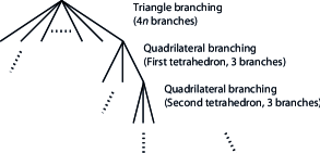
Figure 14. The combinatorial search tree

We arrange these branches into a combinatorial search tree, as illustrated in Figure 14: the triangle branch is chosen first, and then the $n$ quadrilateral branches are chosen in some order (which we describe shortly). To reduce the total amount of branching, we merge quadrilateral branches (a) and (b) into the single branch (a*) $x^{\square}_{t,1}\geq 0$ and $x^{\square}_{t,2}=x^{\square}_{t,3}=0$, so there are only three (not four) branches at each quadrilateral decision.

To run step 1 of Algorithm 9, we begin at the root of this search tree and traverse it in a depth-first fashion. At all stages we maintain a system $\mathcal{N}$ of linear constraints corresponding to the branches that have been chosen:

• At the root of the tree we initialise $\mathcal{N}$ to the constraints $\mathbf{x}\geq 0$, the matching equations $A\mathbf{x}=0$, and $\chi(\mathbf{x})\geq 1$.

• Each time we follow a new branch down, we extend $\mathcal{N}$ by adding additional constraints to describe the branch that was chosen. For instance, when following a triangle branch we would add constraints of the form $x^{\triangle}_{1},\ldots,x^{\triangle}_{i-1}\geq 1$ and $x^{\triangle}_{i}=0$, and when following quadrilateral branch (d) for some tetrahedron we would add the constraints $x^{\square}_{t,3}\geq 1$ and $x^{\square}_{t,1}=x^{\square}_{t,2}=0$.

• Conversely, each time we backtrack and follow a branch up, we remove these additional constraints from $\mathcal{N}$.

Crucially, each time we enter a node in the search tree we test the system $\mathcal{N}$ for feasibility (i.e., whether it has a solution). If the system is not feasible, then we backtrack immediately (since the branches chosen thus far are inconsistent, and cannot lead to a desired admissible point $\mathbf{p}\in\mathbb{R}^{7n}$). If we ever reach a leaf node of the tree—that is, a node at which we have followed a triangle branch plus quadrilateral branches for all $n$ tetrahedra—then any solution to the system $\mathcal{N}$ is the admissible point $\mathbf{p}\in\mathbb{R}^{7n}$ that we require, at which point we can terminate the search and move immediately to step 2 of Algorithm 9.

We emphasise the underlying branch-and-bound motivations behind this search. If we treat $\chi$ as a linear objective function to maximise, then our feasibility tests at each node play the role of linear relaxations—in the absence of constraints for decisions not yet made, they test whether the maximum $\chi$ could possibly be positive in the subtree below the current node.

As is common in branch-and-bound, the order in which we make individual branching decisions can have an enormous impact on the overall running time. With this in mind, we now describe important enhancements to the vertical layout of the search tree, i.e., the order in which we make our $n$ quadrilateral decisions. Figure 14 depicts these decisions as ordered by tetrahedron number; however, we can dynamically reorder these decisions to take full advantage of the interaction between different constraints. Experimentation suggests that the following optimisations are crucial to the polynomial-time behaviour that we observe in practice in Section 4.

• After choosing an initial triangle branch, if the triangle coordinate that we set to zero was in the $i$th tetrahedron, then we immediately branch on quadrilateral coordinates in the same ($i$th) tetrahedron.

  This is because setting a triangle and two quadrilateral coordinates to zero in the same tetrahedron is an extremely powerful constraint, and immediately eliminates several other “nearby” quadrilateral and triangle coordinates from surrounding tetrahedra.

• For subsequent quadrilateral decisions, we greedily branch on the tetrahedron that yields the fewest feasible child nodes. That is, for each unused tetrahedron we build the three constraint systems $\mathcal{N}$ that would result at each of the three child nodes if we branched next on that tetrahedron, and we count how many of these three systems are feasible. We then branch on quadrilateral coordinates in whichever tetrahedron minimises this count.

  Essentially, this greedy approach allows us to lock in additional “forced” constraints as quickly as possible. Moreover, if there is some tetrahedron in which none of the three quadrilateral branches yield a feasible child node, our approach detects this and allows us to backtrack immediately. A drawback of this greedy method is that it requires a linear number of feasibility tests at each node of the search tree, but this only affects the running time by a polynomial factor.

Lemma 10.

Algorithm 9 (which implements the search in step 3 of Algorithm 2) is correct in either finding a connected normal surface $S$ which is not the vertex link and has positive Euler characteristic, or in showing that no such surface exists. Moreover, the algorithm runs in time $O(3^{n}\times\mathrm{poly}(n))$.

Proof.

Recall that step 1 of Algorithm 9 searches for an admissible point $\mathbf{p}\in\mathbb{R}^{7n}$ for which $\chi(\mathbf{p})\geq 1$, and for which at least one of the $4n$ triangle coordinates is zero.

Suppose we fail to find such a point $\mathbf{p}$ in step 1. If there were some connected normal surface $S$ which is not the vertex link and has positive Euler characteristic, then (by Lemma 8) the vector $\mathbf{p}=\mathbf{v}(S)\in\mathbb{R}^{7n}$ would satisfy our search criteria. Therefore the algorithm is correct in concluding that no such surface $S$ exists.

Suppose we do find such a point $\mathbf{p}$ in step 1. Consider now the point $\mathbf{q}$ that we construct in steps 2 and 3 of the algorithm. It is clear that $\mathbf{q}$ exists (i.e., the final system $\mathcal{L}$ is feasible), since the initial system $\mathcal{L}$ has $\mathbf{p}$ as a solution, each additional constraint added in step 2(a) is again satisfied by $\mathbf{p}$, and each additional constraint added in step 2(b) is explicitly tested for feasibility.

We now claim that $\mathbf{q}$ is admissible. This is true because the conditions $\mathbf{q}\geq 0$ and $A\mathbf{q}=0$ are built into the system $\mathcal{L}$; moreover, by step 2(a) we know that each coordinate that is zero in $\mathbf{p}$ is also zero in $\mathbf{q}$, and so because $\mathbf{p}$ satisfies the quadrilateral constraints then $\mathbf{q}$ must also.

We next show that $\mathbf{q}$ scales to a rational vector. Let $\mathcal{P}$ be the rational polyhedron in $\mathbb{R}^{7n}$ defined by the system $\mathcal{L}$. From the structure of the inequalities that define $\mathcal{L}$, we see that each facet of $\mathcal{P}$ is obtained by intersecting $\mathcal{P}$ with a supporting hyperplane of the form (i) $x_{i}=0$, or (ii) $\chi(\mathbf{x})=1$. From step 2 we see that any intersection of $\mathcal{P}$ with a hyperplane $x_{i}=0$ either includes all of $\mathcal{P}$ or is the empty set; either way we cannot obtain a facet. Therefore $\mathcal{P}$ has only one facet (the intersection with $\chi(\mathbf{x})=1$), and it follows that $\mathcal{P}$ is a one-dimensional ray. Since $\mathcal{L}$ is a rational system we conclude that the solution $\mathbf{q}$ scales down to a rational point (the vertex of $\mathcal{P}$ at the beginning of this ray).

It follows that in step 3 the multiple $\lambda\mathbf{q}$ is well-defined, and represents an admissible integer vector with $\chi(\lambda\mathbf{q})>0$. We therefore have $\lambda\mathbf{q}=\mathbf{v}(S)$ for some normal surface $S$ in $\mathcal{T}$ with positive Euler characteristic. Because some triangle coordinate of $\mathbf{p}$ is zero, step 2(a) ensures that some triangle coordinate of $\mathbf{v}(S)$ is zero, and it follows from Lemma 8 that $S$ is not the vertex link.

We now use Lemma 7 to show that this surface is connected. Suppose there were some normal surface $S^{\prime}$ with positive Euler characteristic where (i) for every coordinate of $\lambda\mathbf{q}=\mathbf{v}(S)$ which is zero, the corresponding coordinate of $\mathbf{v}(S^{\prime})$ is likewise zero; and (ii) there is some $i$ for which the $i$th coordinate of $\lambda\mathbf{q}=\mathbf{v}(S)$ is non-zero but the $i$th coordinate of $\mathbf{v}(S^{\prime})$ is zero. Then in step 2(b) of the algorithm, for this particular value of $i$, the constraint $x_{i}=0$ would have given a feasible system (having $\mathbf{v}(S^{\prime})$ as a solution). Therefore $x_{i}=0$ would have been a condition in the final system $\mathcal{L}$, and $\mathbf{q}$ could not have been a solution—a contradiction. Therefore $S$ satisfies the conditions of Lemma 7, and so (because our scaling factor $\lambda$ realises the smallest possible integer multiple) the surface $S$ must be connected.

We now have that $S$ is a connected normal surface which is not the vertex link and which has positive Euler characteristic. This concludes the proof that the output of Algorithm 9 is correct.

To finish, we analyse the time complexity of the algorithm. First we observe that every feasibility test that appears in the algorithm involves a linear number of constraints, each with integer coefficients of size $O(1)$. In particular:

• The system of matching equations $A\mathbf{x}=0$ contains at most $6n$ equations, each of the form $x^{\triangle}_{i}+x^{\square}_{j,k}=x^{\triangle}_{u}+x^{\square}_{v,w}$.

• Recall from the preliminaries section that there are many choices for our linear Euler characteristic function $\chi$. To ensure that this function has constant sized integer coefficients, we choose the formulation $\chi(\mathbf{x})=\chi_{2}(\mathbf{x})-\chi_{1}(\mathbf{x})+\chi_{0}(\mathbf{x})$, where:

  • $\chi_{2}(\mathbf{x})$ is the sum of all coordinates of $\mathbf{x}$;

  • $\chi_{1}(\mathbf{x})=\sum_{F}\chi_{1}^{F}(\mathbf{x})$, where $F$ ranges over all triangular faces $F$ of the triangulation $\mathcal{T}$, and where each $\chi_{1}^{F}(\mathbf{x})$ is computed by choosing an arbitrary tetrahedron $\Delta_{F}$ that contains $F$, and summing the six coordinates of $\mathbf{x}$ that correspond to normal discs in $\Delta_{F}$ that meet $F$;

  • $\chi_{0}(\mathbf{x})=\sum_{e}\chi_{0}^{e}(\mathbf{x})$, where $e$ ranges over all edges of $\mathcal{T}$, and each $\chi_{0}^{e}(\mathbf{x})$ is likewise computed by choosing an arbitrary tetrahedron $\Delta_{e}$ that contains $e$ and summing the four coordinates of $\mathbf{x}$ that correspond to normal discs in $\Delta_{e}$ that meet $e$.

  If some face $F$ appears multiple times within the tetrahedron $\Delta_{F}$ (i.e., two faces of $\Delta_{F}$ are identified together), then we restrict our attention to just one of these appearances when computing $\chi_{1}^{F}(\mathbf{x})$; likewise with $\chi_{0}^{e}(\mathbf{x})$.

  We note that this choice of Euler characteristic function is a valid one: if the vector $\mathbf{x}$ represents a normal surface $S$ then $\chi_{2}(\mathbf{x})$, $\chi_{1}(\mathbf{x})$ and $\chi_{0}(\mathbf{x})$ count the number of discs, edges and vertices respectively in $S$, and so $\chi(\mathbf{x})$ is indeed the Euler characteristic of $S$.

  Regarding the coefficients of this function: since each coordinate of $\mathbf{x}$ may appear in at most four distinct terms $\chi_{1}^{F}(\mathbf{x})$ and at most four distinct terms $\chi_{0}^{e}(\mathbf{x})$, the formulation above expresses $\chi(\mathbf{x})$ as a linear function with integer coefficients all in the range $-3,\ldots,+5$.

This establishes that every feasibility test that appears in the algorithm involves a linear number of constraints each with constant sized coefficients. It follows that every such test can be solved in polynomial time using linear programming techniques.

We can now measure the time complexity of each step of the algorithm:

• For step 1 we simply count nodes: there are $4n$ branches for the initial triangle decision and three branches for each of the $n$ quadrilateral decisions, giving $4n\cdot 3^{n}$ leaf nodes in the worst case. Each feasibility test can be run in polynomial time as noted above, yielding an overall running time of $O(3^{n}\times\mathrm{poly}(n))$.

• Step 2 runs in polynomial time because throughout its evolution the system $\mathcal{L}$ always contains $O(n)$ constraints, we only modify it $O(n)$ times, and for each modification we run a single feasibility test which can be performed in polynomial time as before.

• For step 3 we must show that we can perform the necessary arithmetic on $\mathbf{q}$ in polynomial time. For this it suffices to show that the coordinates of our smallest integer multiple $\lambda\mathbf{q}$ each have just $O(n)$ bits.

  By following the same argument as used in Lemma 7, we find that $\mathbf{q}$ lies on an extreme ray of the polyhedral cone $\mathcal{C}$ defined by $\mathbf{x}\geq 0$ and $A\mathbf{x}=0$. This can also be seen directly: by removing the non-homogeneous constraint $\chi(\mathbf{x})\geq 1$ from the final system $\mathcal{L}$ we extend our one-dimensional solution set to a homogeneous ray in $\mathbb{R}^{7n}$, and by removing the additional constraints $x_{i}=0$ that were added in step 2 we further enlarge this to the full cone $\mathcal{C}$, with our original solution set now on an extreme ray of $\mathcal{C}$.

  We finish by invoking a result of Hass et al. [26, Lemma 6.1], which shows that any extreme ray of $\mathcal{C}$ can be expressed as an integer vector with all coordinates bounded by $\exp(O(n))$—that is, by $O(n)$ bits.

This establishes an overall running time of $O(3^{n}\times\mathrm{poly}(n))$ for Algorithm 9. ∎

We pause to make some final observations on step 1 of Algorithm 9, where we find the point $\mathbf{p}\in\mathbb{R}^{7n}$ using our branching scheme.

• The quadrilateral constraints are special forms of SOS 1 constraints: an SOS 1, or special ordered set of type 1, is a set of variables at most one of which may be non-zero [6]. Thus, in effect, step 1 of Algorithm 9 solves a family of SOS 1 constrained problems using customised branching rules.

• The linear programs that we solve in step 1 of Algorithm 9 do not involve any explicit objective function—we are simply interested in testing feasibility. One could also introduce an explicit objective function in the hope that, if the point $\mathbf{p}$ does exist, then we might find it more quickly. For instance, we could minimise the sum of triangle coordinates (in the hope that one of the $4n$ triangle coordinates might be zero), or minimise the sum of quadrilateral coordinates (in the hope that the quadrilateral constraints might be satisfied).

  However, since such heuristics do not guarantee to satisfy the relevant combinatorial constraints, they are primarily useful only in the cases where $\mathbf{p}$ does exist—that is, where the input knot is trivial and/or the triangulation of the knot complement is “inefficient” (i.e., it can be simplified by crushing). We note that such inputs are often already “easy”, in the sense that they can typically be resolved (or at least reduced) using fast local simplification techniques instead, as mentioned in the introduction.

3.4. Proofs of correctness and running time

Our final task in this section is to tie everything together: we prove that the full unknot recognition algorithm is correct (Theorem 11) and describe its worst-case time complexity (Theorem 12).

Theorem 11 (Correctness).

Algorithm 2 is correct in determining whether the input knot $K$ is trivial or non-trivial.

Proof.

All that remains is to show that the claims made in step 3 of the algorithm (after searching for the normal surface $S$) are correct.

By Theorem 1, it is clear that if no surface $S$ is found then $K$ is non-trivial, and if $S$ is a disc with non-trivial boundary then $K$ is trivial. Otherwise the algorithm tells us to crush $S$, whereupon Lemma 5 shows that the new triangulation $\mathcal{T}^{\prime}$ represents the same knot complement $\overline{K}$ with strictly fewer than $n$ tetrahedra, as claimed. ∎

Theorem 12 (Running time).

Let $c$ be the number of crossings in the input knot diagram for Algorithm 2. With the exception of the search in step 3 (where we search for the normal surface $S$), every step of Algorithm 2 runs in time polynomial in $c$. In contrast, the search in step 3 runs in time $O(3^{n}\times\mathrm{poly}(n))$, where $n\in O(c)$ is the number of tetrahedra in the triangulation $\mathcal{T}$. Every step (including this search) is repeated at most $O(c)$ times.

Proof.

Following Hass et al. [26, Lemma 7.2], step 1 of the algorithm takes $O(c\log c)$ time and builds a triangulation of $\overline{K}$ with $n\in O(c)$ tetrahedra. By Lemma 6, the conversion in step 2 to a one-vertex triangulation then takes $O(c^{3})$ time.

Lemma 10 shows that the search in step 3 runs in time $O(3^{n}\times\mathrm{poly}(n))$. Following this search, the only significant actions are (i) testing whether the boundary of $S$ is non-trivial in $\partial\mathcal{T}$, and (ii) potentially crushing the surface $S$.

Because $\mathcal{T}$ is a one-vertex triangulation, the boundary torus $\partial\mathcal{T}$ contains just two triangles, and the boundary of $S$ follows a non-trivial curve on $\partial\mathcal{T}$ if and only if it is not a trivial loop encircling the (unique) vertex. Therefore we can test $S$ for non-trivial boundary in $O(n)$ time just by examining the coordinates of $\mathbf{v}(S)$. Finally, Lemma 5 shows that we can crush the surface $S$ in $O(n)$ time also.

Each iteration through these steps results in either termination or a reduction in the number of tetrahedra, and so we repeat these steps at most $n\in O(c)$ times. ∎

4. Experimental performance

Here we describe the results of extensive testing of the new unknot recognition algorithm over all $2977$ prime knots with $\leq 12$ crossings.

The algorithm has been implemented in C++ using the open-source computational topology software package Regina [10, 14], and is now built directly into Regina as of version 4.94. We briefly describe some aspects of the implementation, and then describe the experimental data and results.

4.1. Implementation

Although it is possible to test the feasibility of a system of linear constraints in polynomial time (for instance, using interior point methods [23, 33]), we use a variant of the simplex method due to its ease of implementation and its excellent performance in practical settings (as discussed further in Section 6). Specifically, we use the revised dual simplex method [36] with an implementation that exploits the sparseness of the matching equations $A\mathbf{x}=0$.

For a pivoting rule, we use Dantzig’s classical method of choosing the exiting variable with largest magnitude negative value in the tableaux [18]. Although this method is fast and works well to reduce the total number of pivots, it can lead to cycling. We therefore use Brent’s algorithm to detect cycling [8], and when it occurs we switch to Bland’s rule instead [7], which exhibits weaker performance but does not cycle. We note that cycling was detected for some experimental inputs, and so these cycle-breaking techniques are indeed necessary in practice.

All computations use exact integer and rational arithmetic, provided by the GNU multiple precision arithmetic library [22]. To limit the overhead, we work in native integers wherever possible but test for overflow on all arithmetical operations, and only switch to exact arithmetic when necessary. This behaviour, which improves performance surprisingly well, is inspired by (but far less sophisticated than) the lazy evaluation methods used for exact arithmetic in the CGAL computational geometry library [1, 9].

4.2. Experimental results

Our experimental data set consists of all $2977$ prime knots with $\leq 12$ crossings, as taken from the KnotInfo database [17]. This is intended as an exhaustive and “punishing” data set, where simplification tools cannot solve the problems (since the inputs are non-trivial knots), and where our branching search needs to conclusively determine that certain normal surfaces do not exist (so there is no chance for early termination).

As is common in computational topology, our first step before running any other algorithms is to simplify the input triangulations using a suite of local moves; we use the ready-made (and polynomial time) suite from Regina [12].

The resulting triangulations are large, with up to $n=50$ tetrahedra. It is a testament to the strength of the simplification suite that for all $2977$ inputs we only require a single pass through Algorithm 9 (the branching search)—we never need to crush away “junk” discs or spheres and run the search again (as in step 3 of Algorithm 2). Similarly, we find that in practice the simplification suite always produces a one-vertex triangulation immediately, with no need for the complex operations described in Lemma 6.

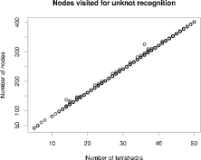
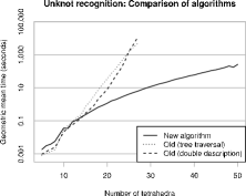
Figure 15. Performance summary for unknot recognition

The first plot of Figure 15 counts how many nodes the new algorithm visits in the branching search tree (as described in Section 3.3); this measure is crucial because it determines how many linear programming problems we solve, and is the source of the worst-case exponential running time. The results are unequivocally linear: in every case the number of nodes lies between $8n$ and $10n$, and for all but 24 of the inputs the figure is precisely $8n+1$ (the smallest possible, indicating that we never need to branch on quadrilateral coordinates at all). This linear growth in the number of nodes corresponds to a polynomial running time, and explains the exceptional performance of the algorithm.

The second plot of Figure 15 measures running times, comparing the new algorithm against prior state-of-the-art algorithms that rely on an enumeration of candidate normal discs. These prior algorithms use two different enumeration techniques: one based on the double description method [11], and one based on a more recent tree traversal method [16]. These prior algorithms are also implemented in Regina, and their code is heavily optimised; see [12] for an overview of each.

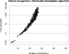
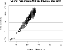
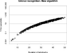
Figure 16. Detailed running times for unknot recognition on the first 2977 prime knots

All running times are single-threaded (measured on a 2.93 GHz Intel Core i7); note that the time axis in the plot is logarithmic. The summary plot in Figure 15 aggregates all running times for each number of tetrahedra $n$ using the geometric mean (which benefits the older algorithms, since they have much wider variability). Figure 16 shows the individual running times for every input under each algorithm.

The results are striking. When viewed on this log scale, the linear profiles of the older algorithms indicate a clear exponential-time behaviour. Moreover, for these older algorithms we could only use the first $515$ input knots (as sorted by increasing $n$), because running times became too large to proceed any further—a linear regression on $\log(\mathrm{time})$ suggests that for the largest case with $n=50$ the older tree traversal algorithm would take $\sim 6000$ years, and the older double description method would take $\sim 40,000$ years. In contrast, the new algorithm solved all $2977$ input cases (including the largest case with $n=50$) in under 5 minutes each.

5. 3-sphere recognition and prime decomposition

Looking beyond unknot recognition, we can adapt our new algorithm for other topological problems, such as 3-sphere recognition and prime decomposition. We briefly sketch the key ideas here.

Given a triangulation $\mathcal{T}$ that represents a closed orientable 3-manifold, 3-sphere recognition asks whether this manifold is topologically equivalent to the 3-sphere, and prime decomposition breaks this 3-manifold into a collection of “prime factors” (which combine to make the original manifold using the topological operation of connected sum).

For both problems, early algorithms were mathematical breakthroughs but algorithmically cumbersome and impractical to implement [32, 42]. They have since enjoyed great improvements in both implementability and efficiency, but like unknot recognition they still require worst-case exponential time. See [12] for a modern formulation of these algorithms as they appear today.

For both algorithms, the central operations—and their exponential-time bottlenecks—are steps that search for normal or “octagonal almost normal” spheres within a triangulation $\mathcal{T}$. An octagonal almost normal surface is like a normal surface, but in addition to triangles and quadrilaterals we require precisely one octagonal piece in precisely one tetrahedron.

We can adapt Algorithm 9 (our new search based on branching and feasibility tests) for these tasks. To locate normal spheres, we can essentially use Algorithm 9 as it stands; to locate almost normal spheres, we use a variant that works with a different coordinate system (which supports octagonal pieces). These new search procedures can be dropped directly into modern 3-sphere recognition and prime decomposition implementations [12].

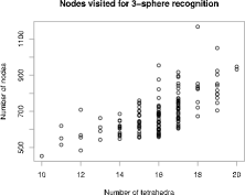
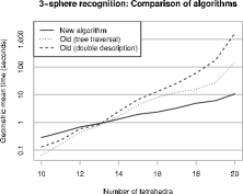
Figure 17. Performance summary for 3-sphere recognition

As before, we empirically test our new algorithm for 3-sphere recognition over a comprehensive and “punishing” data set. This time our test inputs are the first $150$ homology spheres in the Hodgson-Weeks census [27]; again, since none of the inputs are 3-spheres, these are difficult cases to solve: simplification tools cannot solve the problem alone, and there is no opportunity for early termination of our branching search.

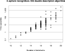
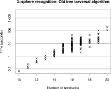
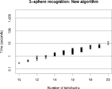
Figure 18. Detailed running times for 3-sphere recognition on the first 150 homology spheres

The triangulations of these homology spheres have up to $n=20$ tetrahedra. Figure 17 shows the number of nodes visited in the search tree for each input, and summarises the performance of the old and new algorithms. Figure 18 shows detailed running times for each input case.

The results for 3-sphere recognition are less clear-cut than for unknot recognition, and no longer exhibit a polynomial-time profile; we expect this is due to the introduction of almost normal surfaces. Nevertheless, the results are still extremely pleasing. The new algorithm, though slower for small cases, becomes markedly faster than the prior algorithms as $n$ increases. For the final case ($n=20$), the new algorithm runs over $15$ times faster than the prior tree traversal algorithm and roughly $223$ times faster than the prior double description algorithm. Furthermore, as is evident from Figure 18, the new algorithm exhibits much less variability in running times.

We do not test the prime decomposition algorithm separately. This is essentially because the prime decomposition algorithm appears as a sub-component of 3-sphere recognition (which we have already tested above); see [12, 31] for details.

6. Discussion

Although our new algorithm for unknot recognition remains exponential time in theory, the observed polynomial growth in practice is extremely pleasing, and indeed very exciting—this moves the study of unknot recognition into a new phase, where we can now solve it conclusively and quickly “in practice”, albeit without theoretical guarantees on the running time. This is reminiscent of the simplex method for linear programming, an algorithm that requires exponential time in the worst case but which, despite the existence of polynomial-time alternatives [23, 33], still enjoys widespread use because of its extremely fast “typical” behaviour in practice.

We have a good understanding of why the simplex method works well in practice: it has been shown to be polynomial time in settings such as average, generic and smoothed complexity [43, 44, 45]. In contrast, there are no such results for unknot recognition; more generally, average, generic and smoothed results are extremely scarce in the study of topological algorithms on 3-dimensional triangulations (the setting for this and many other knot algorithms). Reasons include:

• Combinatorial models of random triangulations produce an overwhelming amount of “junk”: the probability that a random pairwise gluing of faces from $n$ tetrahedra yields a 3-manifold triangulation tends to zero as $n\to\infty$ [20], and there is no known polynomial-time algorithm for sampling a random 3-manifold triangulation [41].

• “Walking” through the space of 3-manifold triangulations is difficult because the diameter of this space could be extremely large: for knot complements the best known bounds involve exponentially high towers of exponentials [39].

In Section 5 we showed how to adapt this new unknot recognition algorithm to the problems of 3-sphere recognition and prime decomposition. Looking further, these techniques have potential to extend to an even broader range of topological problems: promising candidates include 0-efficiency algorithms [31], and the difficult but important problem of finding incompressible surfaces [30].

Of course knots and their complements can grow significantly larger than 12 crossings and 50 tetrahedra, and it is difficult to know whether the consistent polynomial-time behaviour seen in our experiments is maintained as $n$ grows. As an initial exploration into this, we have run the same experiments over the 20-crossing dodecahedral knots $D_{f}$ and $D_{s}$ [4]. These are larger knots that exhibit remarkable properties [40], and that lie well beyond the scope of the KnotInfo database.

For both $D_{f}$ and $D_{s}$ we see the same polynomial-time profile as in our earlier experiments. The knot complements have $n=72$ and $n=73$ tetrahedra (so the algorithm works in vector spaces of dimension $504$ and $511$ respectively), and for both knots Algorithm 2 visits precisely $8n+1$ nodes in the search tree (the smallest possible, as discussed in Section 4.2). Both running times are under half an hour.

It seems reasonable to believe that pathological inputs should exist that force Algorithm 2 to traverse a genuinely exponential search tree (just as, for the simplex method, it is possible to build pathological linear programs that require an exponential number of pivots [34]). However, it remains a considerable ongoing challenge to find them.

References

- [1] Cgal, Computational Geometry Algorithms Library, http://www.cgal.org/.
- [2] Colin C. Adams, The knot book: An elementary introduction to the mathematical theory of knots, W. H. Freeman & Co., New York, 1994.
- [3] Ian Agol, Thurston norm is polynomial time certifiable, slides previously available from http://homepages.math.uic.edu/~agol/coNP/coNP01.html, 2002.
- [4] I. R. Aitchison and J. H. Rubinstein, Combinatorial cubings, cusps, and the dodecahedral knots, Topology ’90 (Columbus, OH, 1990), Ohio State Univ. Math. Res. Inst. Publ., vol. 1, de Gruyter, Berlin, 1992, pp. 17–26.
- [5] M. V. Andreeva, I. A. Dynnikov, and K. Polthier, A mathematical webservice for recognizing the unknot, Mathematical Software: Proceedings of the First International Congress of Mathematical Software, World Scientific, 2002, pp. 201–207.
- [6] E. M. L. Beale and J. A. Tomlin, Special facilities in a general mathematical programming system for nonconvex problems using ordered sets of variables, Proceedings of the Fifth International Conference on Operational Research (J. Lawrence, ed.), Tavistock Publications, 1970, pp. 447–454.
- [7] Robert G. Bland, New finite pivoting rules for the simplex method, Math. Oper. Res. 2 (1977), no. 2, 103–107.
- [8] Richard P. Brent, An improved Monte Carlo factorization algorithm, BIT 20 (1980), no. 2, 176–184.
- [9] Hervé Brönnimann, Christoph Burnikel, and Sylvain Pion, Interval arithmetic yields efficient dynamic filters for computational geometry, Discrete Appl. Math. 109 (2001), no. 1-2, 25–47.
- [10] Benjamin A. Burton, Introducing Regina, the 3-manifold topology software, Experiment. Math. 13 (2004), no. 3, 267–272.
- [11] by same author, Optimizing the double description method for normal surface enumeration, Math. Comp. 79 (2010), no. 269, 453–484.
- [12] by same author, Computational topology with Regina: Algorithms, heuristics and implementations, Geometry and Topology Down Under (Craig D. Hodgson, William H. Jaco, Martin G. Scharlemann, and Stephan Tillmann, eds.), Contemporary Mathematics, no. 597, Amer. Math. Soc., Providence, RI, 2013.
- [13] by same author, A new approach to crushing 3-manifold triangulations, Discrete Comput. Geom. 52 (2014), no. 1, 116–139.
- [14] Benjamin A. Burton, Ryan Budney, William Pettersson, et al., Regina: Software for 3-manifold topology and normal surface theory, http://regina.sourceforge.net/, 1999–2014.
- [15] Benjamin A. Burton and Melih Ozlen, Computing the crosscap number of a knot using integer programming and normal surfaces, ACM Trans. Math. Software 39 (2012), no. 1, 4:1–4:18.
- [16] by same author, A tree traversal algorithm for decision problems in knot theory and 3-manifold topology, Algorithmica 65 (2013), no. 4, 772–801.
- [17] Jae Choon Cha and Charles Livingston, KnotInfo: Table of knot invariants, http://www.indiana.edu/~knotinfo, accessed June 2011.
- [18] George B. Dantzig, Linear programming and extensions, Princeton University Press, Princeton, N.J., 1963.
- [19] Nathan M. Dunfield and Anil N. Hirani, The least spanning area of a knot and the optimal bounding chain problem, SCG ’11: Proceedings of the Twenty-Seventh Annual Symposium on Computational Geometry, ACM, 2011, pp. 135–144.
- [20] Nathan M. Dunfield and William P. Thurston, Finite covers of random 3-manifolds, Invent. Math. 166 (2006), no. 3, 457–521.
- [21] I. A. Dynnikov, Recognition algorithms in knot theory, Uspekhi Mat. Nauk 58 (2003), no. 6(354), 45–92.
- [22] Torbjörn Granlund et al., The GNU multiple precision arithmetic library, http://gmplib.org/, 1991–2010.
- [23] L. G. Hačijan, A polynomial algorithm in linear programming, Dokl. Akad. Nauk SSSR 244 (1979), no. 5, 1093–1096.
- [24] Wolfgang Haken, Theorie der Normalflächen, Acta Math. 105 (1961), 245–375.
- [25] Joel Hass, New results on the complexity of recognizing the 3-sphere, Oberwolfach Rep. 9 (2012), no. 2, 1425–1426.
- [26] Joel Hass, Jeffrey C. Lagarias, and Nicholas Pippenger, The computational complexity of knot and link problems, J. Assoc. Comput. Mach. 46 (1999), no. 2, 185–211.
- [27] Craig D. Hodgson and Jeffrey R. Weeks, Symmetries, isometries and length spectra of closed hyperbolic three-manifolds, Experiment. Math. 3 (1994), no. 4, 261–274.
- [28] Jim Hoste, The enumeration and classification of knots and links, Handbook of Knot Theory, Elsevier B. V., Amsterdam, 2005, pp. 209–232.
- [29] William Jaco, David Letscher, and J. Hyam Rubinstein, Algorithms for essential surfaces in 3-manifolds, Topology and Geometry: Commemorating SISTAG, Contemporary Mathematics, no. 314, Amer. Math. Soc., Providence, RI, 2002, pp. 107–124.
- [30] William Jaco and Ulrich Oertel, An algorithm to decide if a -manifold is a Haken manifold, Topology 23 (1984), no. 2, 195–209.
- [31] William Jaco and J. Hyam Rubinstein, 0-efficient triangulations of 3-manifolds, J. Differential Geom. 65 (2003), no. 1, 61–168.
- [32] William Jaco and Jeffrey L. Tollefson, Algorithms for the complete decomposition of a closed -manifold, Illinois J. Math. 39 (1995), no. 3, 358–406.
- [33] N. Karmarkar, A new polynomial-time algorithm for linear programming, Combinatorica 4 (1984), no. 4, 373–395.
- [34] Victor Klee and George J. Minty, How good is the simplex algorithm?, Inequalities, III (Proc. Third Sympos., Univ. California, Los Angeles, Calif., 1969), Academic Press, New York, 1972, pp. 159–175.
- [35] Greg Kuperberg, Knottedness is in , modulo GRH, Adv. Math. 256 (2014), 493–506.
- [36] C. E. Lemke, The dual method of solving the linear programming problem, Naval Res. Logist. Quart. 1 (1954), 36–47.
- [37] W. B. Raymond Lickorish, An introduction to knot theory, Graduate Texts in Mathematics, no. 175, Springer, New York, 1997.
- [38] Sergei V. Matveev, Complexity theory of three-dimensional manifolds, Acta Appl. Math. 19 (1990), no. 2, 101–130.
- [39] Aleksandar Mijatović, Simplical structures of knot complements, Math. Res. Lett. 12 (2005), no. 5-6, 843–856.
- [40] Walter D. Neumann and Alan W. Reid, Arithmetic of hyperbolic manifolds, Topology ’90 (Columbus, OH, 1990), Ohio State Univ. Math. Res. Inst. Publ., vol. 1, de Gruyter, Berlin, 1992, pp. 273–310.
- [41] Vic Reiner and John Sullivan, Triangulations: Minutes of the open problem session, Oberwolfach Rep. 9 (2012), no. 2, 1478–1481.
- [42] J. Hyam Rubinstein, An algorithm to recognize the -sphere, Proceedings of the International Congress of Mathematicians (Zürich, 1994), vol. 1, Birkhäuser, 1995, pp. 601–611.
- [43] Steve Smale, On the average number of steps of the simplex method of linear programming, Math. Programming 27 (1983), no. 3, 241–262.
- [44] Daniel Spielman and Shang-Hua Teng, Smoothed analysis of algorithms: Why the simplex algorithm usually takes polynomial time, Proceedings of the Thirty-Third Annual ACM Symposium on Theory of Computing, ACM, 2001, pp. 296–305.
- [45] A. M. Vershik and P. V. Sporyshev, Estimation of the mean number of steps in the simplex method, and problems of asymptotic integral geometry, Dokl. Akad. Nauk SSSR 271 (1983), no. 5, 1044–1048.