Spin dynamics of hard-soft magnetic multi-layer systems: effect of Exchange, Dipolar and Dzyaloshinski-Moriya interactions

Abstract

We investigate the effect of coupling (intensity and nature), applied field, and anisotropy on the spin dynamics of a multi-layer system composed of a hard magnetic slab coupled to a soft magnetic slab through a nonmagnetic spacer. The soft slab is modeled as a stack of several atomic layers while the hard layer, of a different material, is either considered as a pinned macroscopic magnetic moment or as an atomic multi-layer system. We compute the magnetization profile and hysteresis loop of the multi-layer system by solving the Landau-Lifshitz equations for the net magnetic moment of each (atomic) layer. We study the competition between the intra-layer anisotropy and exchange interaction, applied magnetic field, and the inter-slab exchange, dipolar or Dzyaloshinski-Moriya interaction. Comparing the effects on the magnetization profile of the three couplings shows that despite the strong effect of the exchange coupling, the dipolar and Dzyaloshinski-Moriya interactions induce a slight (but non negligible) deviation in either the polar or azimuthal direction thus providing more degrees of freedom for adjusting the spin configuration in the multi-layer system.

I Introduction

Although the “nano-rush” tends to dominate the realm of technological applications, especially magnetic recording, multi-layer magnetic systems benefit from a growing interest in this area mainly due to their high performance (E. F. Kneller and R. H. Hawig, 1991; R. H. Victora, X. Shen, 2005; D. Suess, T. Schrefl, R. Dittrich, M. Kirschner, F. Dorfbauer, G. Hrkac, J. Fidler, 2005). On the other hand, magnetic multi-layer systems and thin films benefit from the acquired long-standing experience and know-how both in growth and characterization leading to a good control of the relevant intrinsic parameters (dimensionality and anisotropy). Moreover, there are many well-established techniques for precise measurements, such as FMR (K.B. Urquhart, B. Heinrich, J.F. Cochran, A.S. Arrott, and Myrtle, 1988; B. Heinrich and J.F.C. Cochran, 1993; B. Heinrich, 1994; Farle, 1998; G. Woltersdorf and Ch. H. Back, 2007), BLS (J.F. Cochran, 1994; C. Mathieu et al., 1998), and the ever developing optical techniques (E. Beaurepaire, J.-C. Merle, A. Daunois, and J.-Y. Bigot, 1996; B. Koopmans, M. van Kampen, J. T. Kohlhepp, and W. J. M. de Jonge, 2000; M. van Kampen, C. Jozsa, J. T. Kohlhepp, P. LeClair, W. J. M. de Jonge, and B. Koopmans, 2002; J. Stöer and H. C. Siegmann, 2006), to cite a few.

The magnetization dynamics of laterally confined elements of alternating magnetic and nonmagnetic layers exhibits a large variety of interesting phenomena for both applications and fundamental research. In this context, theory has to play its usual role of providing reasonable models for interpreting the observed phenomena and suggesting new experiments. An issue of particular interest in this context concerns the coupling in multi-layer systems (P. Bruno, 1995). The inter-layer coupling determines the mechanisms of transport and propagation of a stimulus applied at one end of the structure and the mechanism of the adjustment of magnetic configurations in metallic multi-layer systems by an external magnetic field. In the context of perpendicular magnetic recording with exchange-spring media, improved write-ability is achieved by appropriately tuning the coupling between the soft and hard magnetic layers R. H. Victora, X. Shen (2005); J. P. Wang, W. K. Shen, J. M. Bai, R. H. Victora, J. H. Judy, and W. L. Song (2005); D. Suess, T. Schrefl, S. Faehler, M. Kirschner, G. Hrkac, F. Dorfbauer, and J. Fidler (2005); D. Suess, T. Schrefl, M. Kirschner, G. Hrkac, F. Dorfbauer, O. Ertl, and J. Fidler (2005); K. C. Schuermann, J. D. Dutson, S. Z. Wu, S. D. Harkness, B. Valcu, H. J. Richter, R. W. Chantrell, and K. O’Grady (1993); A. Berger, N. Supper, Y. Ikeda, B. Lengsfield, A. Moser, and E. E. Fullerton (2008). Therefore, it is of paramount importance to fathom the nature of interaction acting at the interface and the role it plays in conveying any perturbation through the multi-layer system. There is a great amount of published work investigating the inter-layer coupling and its effects on the magnetic properties E. W. Hill, S. L. Tomlinson, J.-P. Li (1993); Vargas and Altbir (2000); K. Xia, W. Zhang, M. Lu, and H. Zhai (1997); B. Heinrich et al. (2003); G. N. Kakazei, Yu. G. Pogorelov, M. D. Costa, V. O. Golub, J. B. Sousa, P. P. Freitas, S. Gardoso, and P. E. Wigen (1926); B. Skubic et al. (2006); G. Woltersdorf and Ch. H. Back (2007); M. Madami et al. (2008); L. Sun et al. (2011). For instance, in Ref. G. Woltersdorf and Ch. H. Back, 2007 the authors investigated the magnetization dynamics due to spin currents in magnetic double layers and argued that transport in this structure is governed by a kind of long-range interaction called the dynamic exchange coupling. The microscopic mechanism underlying this effective coupling and the way it affects the collective behavior of magnetic hybrid structures require further investigation. While the RKKY coupling provides an interpretation of experiments on very thin conducting spacers assuming a high degree of perfection (C. Lacroix, B. Dieny, J. P. Gavigan, and D. Givord, 1990), rough surfaces may induce strong stray fields and thereby dipolar coupling in multi-layer systems. For a magnetic bi-layer several configurations are considered in Refs. Vargas and Altbir, 2000; Y. Wang, P. M. Levy, and J. L. Fry, 1990; D. Altbir, M. Kiwi, R. Ramírez, and I. K. Schuller, 1995; D. M. Edwards, R. P. Erickson, J. Mathon, R. B. Muniz, and M. Villeret, 1995. In particular, in Ref. Vargas and Altbir, 2000 the calculations confirm the fact that in the absence of roughness the dipolar coupling between two perfectly flat infinite planes vanishes and that for planes of finite dimensions the dipolar coupling may give rise to a ferromagnetic or an anti-ferromagnetic coupling. On the other hand, one cannot exclude the Dzyaloshinski-Moriya interaction, which is an anti-symmetrical exchange interaction and mainly stems from a combination of low symmetry and spin-orbit coupling (I. Dzyaloshinsky, 1958; T. Moriya, 1960). In the presence of disorder, especially at the interface of thin films or multi-layer systems, the Dzyaloshinski-Moriya interaction has been shown to play an important role since local symmetry is broken by surface effects. Indeed, it leads to large anisotropy and may even change the magnetic order, see Ref. (I. Dzyaloshinsky, 1958; T. Moriya, 1960; A. Crépieux and C. Lacroix, 1998; T. Moriya, 1960). In particular, it has been shown that the Dzyaloshinski-Moriya interaction is induced by spin-orbit coupling between two ferromagnetic layers separated by a paramagnetic layer (K. Xia, W. Zhang, M. Lu, and H. Zhai, 1997).

In the present work, we bring a new contribution that attempts to further clarify the role of three inter-slab couplings, namely exchange, dipolar and Dzyaloshinski-Moriya, in the spin dynamics and magnetization profile (MP). It is also essential to compare these interactions with respect to their efficiency in the realignment of the spin configurations and eventually the magnetization reversal. More precisely, we investigate the effect of coupling (intensity and nature), applied field, and anisotropy on the spin dynamics of a multi-layer system composed of a hard magnetic slab coupled to a soft magnetic slab through a nonmagnetic spacer. The soft slab is modeled as an array of several atomic layers while the hard layer, of a different material, is either considered as a pinned macroscopic magnetic moment or as an array of atomic planes. We compute the magnetization profile and hysteresis loop of the whole system by solving the (coupled) Landau-Lifshitz equations for the net magnetic moment of each (atomic) layer.

This paper is organized as follows. After the introduction we define the system we study in section II. In section III we deal analytically and numerically with the rigid interface. Section IV deals with the soft interface. It presents the results for the effects of applied field, inter-slab couplings, and their comparison. It ends with the results of hysteresis loops. We finally summarize the main results in the conclusion and give a few perspectives for future investigations.

II Statement of the problem

We consider the coupling between two slabs: one is a sufficiently thin hard magnetic system (HMS) with strong out-of-plane anisotropy and, on top of it, a thick soft magnetic system (SMS) with in-plane anisotropy. The SMS slab will be modeled as a multi-layer system of atomic planes of e.g. Fe, whereas the HMS slab will be modeled either as i) a single macroscopic magnetic moment in which case we have a rigid interface (RI), see Fig. 1(a) or as ii) a multi-layer system of atomic planes of e.g. FePt, and in this case we get a relaxed or soft interface (SI), see Fig. 1(b). In both cases, i.e. SMS /HMS-RI or SMS/HMS-SI we have an exchange-spring system with a characteristic MP that depends on various physical parameters such as the SMS-HMS coupling, the anisotropy and exchange coupling within each slab, and the applied field. Accordingly, in this work, we will investigate the effects of these parameters on the MP in the whole system and on the hysteresis loop for the two configurations. In particular, we will consider and compare the effects of three kinds of inter-slab couplings, which are exchange, dipole-dipole and Dzyaloshinski-Moriya. For later reference, we denote by EI-ES, DDI-ES, and DMI-ES the exchange-spring system where SMS and HMS are respectively coupled by exchange interaction (EI), dipole-dipole interaction (DDI), or Dzyaloshinski-Moriya interaction (DMI).

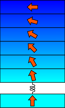
(a) Rigid interface

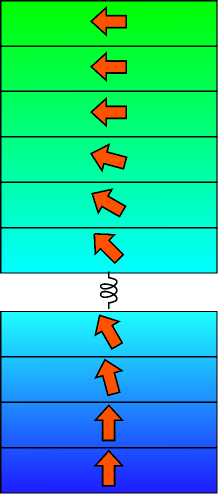
(b) Soft interface

Figure 1: Scheme of a hard/soft coupled bi-layer system

In Ref. (A. F. Franco, J. M. Martinez, J. L. Déjardin, and H. Kachkachi, 2011) the relatively simpler case was considered where both the SMS and HMS were represented by their respective net magnetic moments. The relaxation processes of the corresponding magnetic dimer were then studied. In particular, the relaxation rates related with the reversal of its magnetization were computed. Moreover, the effects of the three couplings mentioned above were investigated for different configurations of the anisotropy easy axes, and at finite temperature. In the present work, we are interested in the exchange-spring effect and in the MP at equilibrium and at zero temperature. Therefore, the main objective here is to investigate how the magnetic structure/state of the SMS adapts to a change in the physical parameters, especially at the interface.

III Rigid interface : numerical versus analytical calculations

III.1 Magnetization profile of the multi-layer system

The exact solution for the MP has been obtained for the system with RI, in the absence of the external magnetic field (de Sousa et al., 2010). For definiteness, the SMS-HMS lies on the $xy$ plane and the out-of-plane anisotropy in the HMS slab points in the $z$ direction. We denote the (net) magnetic moments of HMS by $\bm{\mathbf{\sigma}}$, and the $\mathcal{N}_{s}$ magnetic moments of the SMS by $\mathbf{s}_{i},i=1...,\mathcal{N}_{s}$. Therefore, there is a total of $\mathcal{N}_{s}+1$ magnetic moments in the system pictured here as an open chain of coupled magnetic moments. Indeed, it is assumed that all atomic magnetic moments of each sub-layer $i$ in the SMS are parallel to each other so that their magnetic state can be represented by the net (normalized) magnetic moment $\mathbf{s}_{i}$. Hence, we do not include boundary effects in this study. For the HMS, $\bm{\mathbf{\sigma}}$ represents the net magnetic moment of the whole slab. The system setup is shown in Fig. 2.

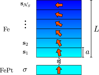
Figure 2: Setup of the SMS/HMS system with rigid interface.

If we denote by $\mathbf{e}_{h}$ the anisotropy easy axis (along the $z$ axis) of HMS and $\mathbf{e}_{s}$ the anisotropy easy axis, taken here along the $x$ axis, of the SMS, the total energy of the system can be written as

$$E=E_{\mathrm{SMS}}+E_{\mathrm{HMS}}+E_{\mathrm{Int}},$$

with

$$E_{\mathrm{SMS}} =-D_{s}\sum_{i=1}^{\mathcal{N}_{s}}\left(\mathbf{s}_{i}^{x}\right)^{2}-J_{s}\sum_{i=1}^{\mathcal{N}_{s}-1}\mathbf{s_{i}}\cdot\mathbf{s}_{i+1}$$

being the energy of the SMS slab. The first term is the in-plane anisotropy with constant $D_{\mathrm{s}}$ (s stands for soft), the second term is intra-SMS nearest-neighbor exchange coupling, of intensity $J_{s}$. Similarly, the energy of the HMS slab contains the out-of-plane anisotropy contribution and the exchange coupling. However, in the present case of a RI, the energy coupling is dropped since we assume that all atomic magnetic moments within the slab are already tightly bound together by the exchange coupling. On the other hand, the anisotropy contribution is also dropped because it is assumed to be strong enough to pin the macroscopic magnetic moment $\bm{\mathbf{\sigma}}$ in the $z$ direction.

Finally, the interaction between the two slabs will be denoted in the sequel by $\lambda$ and will be of three different origins : exchange, dipolar or Dzyaloshinski-Moriya. In the present case, $\lambda$ is the exchange coupling and will be set to $J_{0}$, so that

$$E_{\mathrm{Int}}=-\lambda\bm{\mathbf{\sigma}}\cdot\mathbf{s}_{1}=-J_{0}\bm{\mathbf{\sigma}}\cdot\mathbf{s}_{1}.$$

The analytical solution of the problem requires an additional simplification that consists in setting $J_{0}=J_{s}\equiv J$. Therefore, we can write the energy (in units of exchange coupling) as

$$\mathcal{E}\equiv\frac{E}{J} = -d_{s}\sum_{i=1}^{\mathcal{N}_{s}}\left(\mathbf{s}_{i}^{x}\right)^{2}-\sum_{i=1}^{\mathcal{N}_{s}-1}\bm{s}_{i}\cdot\mathbf{s}_{i+1}-\bm{\mathbf{\sigma}}\cdot\mathbf{s}_{1}$$ (1)

where we have introduced the dimensionless parameter $d_{s}\equiv D_{s}/J_{s}$.

Then, we introduce the coordinate $z$ of each atomic sub-layer along the $z$ direction, such that $z=0$ and $z=L$ represent the sub-layers at the interface and the top of the SMS slab, with $L$ being the thickness of the SMS slab and $a$ that of its atomic sub-layers, i.e. $L=a(\mathcal{N}_{s}-1)$. Note that $i=0$ represents the HMS slab and a slight shift of $0.5a$ in the reference frame between the numerical and the analytical calculations should be taken into account. Indeed, the analytical calculations were performed in the continuum limit. Moreover, the angle deviation with respect to the $z$ axis $\theta_{i}-\theta_{i+1}$ of two adjacent magnetic moments $\bm{s}_{i},\bm{s}_{i+1}$ is supposed to be small. For convenience, we denote $\xi_{i}\equiv\theta_{i}-\theta_{e}$, where $\theta_{e}$ is the equilibrium polar angle of the multilayer system as defined in de Sousa et al. (2010). For typical materials $d_{s}\ll 1$, thus $\theta_{e}\simeq 0$. In such a case one can write down the (finite-difference) equation for $\xi$ from the energy minimization. The solution of this equation can be written as de Sousa et al. (2010)

$$\begin{array}[]{lll}z&=&\int_{0}^{\xi}\!\frac{d\eta}{\sqrt{C_{L}+d_{s}\cos 2\eta}},\\ \\ C_{L}&=&\left(d_{s}\sin 2\xi_{L}\right)^{2}-d_{s}\cos 2\xi_{L},\end{array}$$ (2)

$\xi_{L}$ being the angle deviation of the SMS top sub-layer, i.e. for $z=L$ and is given through the relation

$$L=\intop_{0}^{\xi_{L}}\frac{d\xi}{\sqrt{C_{L}+d_{s}\cos 2\xi}}.$$ (3)

There is a minimal number of sub-layers of the SMS slab, $\mathcal{N}_{s}^{\mathrm{min}}$, or length of the chain, $L^{\mathrm{min}}$, necessary for an onset of noncolinearities of the magnetic moments $s_{i}$. In Ref. de Sousa et al., 2010, $\mathcal{N}_{s}^{\mathrm{min}}$ was found to be given by

$$\mathcal{N}_{s}^{\mathrm{min}}\simeq\frac{\pi}{2\sqrt{2d_{s}}}.$$ (4)

This yields, for instance, $\mathcal{N}_{s}^{\mathrm{min}}\simeq 11$ for $d_{S}=0.01$.

III.2 Magnetization profile of the exchange spring: numerical solution

In order to obtain the MP for the system described above, we solve the set of coupled Landau-Lifshitz equations (LLE)

$$\frac{1}{\gamma}\frac{d\mathbf{s}_{i}}{dt}=\mathbf{s}_{i}\times\mathbf{h}_{i}^{\mathrm{eff}}-\alpha\mathbf{s}_{i}\times\left(\mathbf{s}_{i}\times\mathbf{h}_{i}^{\mathrm{eff}}\right),$$ (5)

where $\mathbf{h}_{i}^{\mathrm{eff}}=-\delta\varepsilon/\delta\mathbf{s}_{i}$ is the (dimensionless) effective field comprising the anisotropy and exchange contributions, together with the interaction at the interface. $\alpha$ is the phenomenological damping parameter, set here to $0.01$. In these zero-temperature calculations, damping is used to drive the system into the equilibrium state, i.e. the state of minimal energy. We start from a state of homogeneous magnetization along the HMS anisotropy axis and allow the system to relax towards a minimum that yields the MP of the system.

In Fig. 3 we plot the angle deviation $\xi^{\mathrm{s}}_{L}$ of the magnetic moment of the top SMS sub-layer against the number of sub-layers in the SMS slab. The results for three values of the in-plane anisotropy $d_{s}$ show a good agreement between our numerical results and Eq. (3).

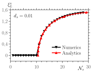
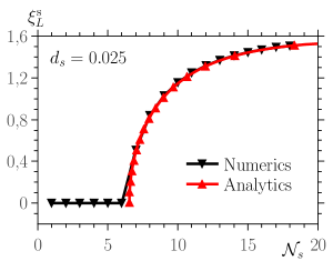
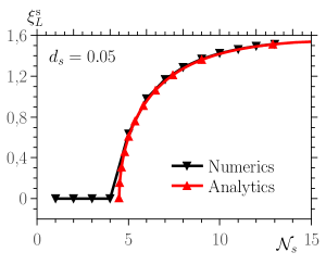
Figure 3: Comparison between analytical and numerical calculations of the magnetization of the top sub-layer $\xi_{L}^{\mathrm{s}}$ for various values of the SMS in-plane anisotropy, $d_{s}=0.01$ (left), $d_{s}=0.025$ (middle), $d_{s}=0.05$ (right).

One can also see how $\mathcal{N}_{\mathrm{min}}$ depends on $d_{s}$ through Eq. (4). For a weak $d_{s}$ the system behavior is dominated by the fixed magnetic moment of the HMS slab through the interface exchange coupling. Adding more sub-layers to the SMS slab attenuates this effect since the interface interaction is counter-balanced by the anisotropy and intra-layer interaction of each SMS sub-layer, leading eventually to a deviation of the magnetic moment of the top SMS sub-layer for $\mathcal{N}\geq\mathcal{N}_{\mathrm{min}}$. On the other hand, when $d_{s}$ increases, the contribution of each SMS sub-layer to the energy of the whole system increases, thus leading to a smaller $\mathcal{N}_{\mathrm{min}}$.

IV Soft interface

In the previous section, we defined a model for a system with rigid interface and energy given by Eq. (1). The agreement with the previously published analytical work validates the numerical approach used here, which can now be employed to deal with more complex systems that are difficult to tackle analytically.

More precisely, we extend the previous model by replacing the macroscopic magnetic moment $\bm{\mathbf{\sigma}}$ of the HMS, that was pinned along the anisotropy direction, by $\mathcal{N}_{h}$ sub-layers each with an out-of-plane (in the $z$ direction) uniaxial anisotropy of intensity $D_{h}$. Moreover, in the present case we apply an external magnetic field $H$ at an angle $\theta_{H}$ with respect to the $z$ axis. Now, within the HMS slab, and similarly to the SMS slab, each sub-layer of index $k$ carries a magnetic moment $\bm{\sigma}_{k}$ with $k=1,\ldots,\mathcal{N}_{h}$, see Fig. 4.

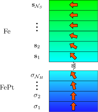
Figure 4: Setup of the SMS/HMS system with soft interface.

The energy of this model then reads

$$E=E_{\mathrm{SMS}}+E_{\mathrm{HMS}}+E_{\mathrm{Int}},$$

with

$$E_{\mathrm{SMS}} =-\mu_{s}H\sum_{i=0}^{\mathcal{N}_{s}}\mathbf{s}_{i}\cdot\mathbf{e}_{H}-D_{s}\sum_{i=1}^{\mathcal{N}_{s}}\left(\mathbf{s}_{i}^{x}\right)^{2}-J_{s}\sum_{i=1}^{\mathcal{N}_{s}-1}\mathbf{s}_{i}\cdot\mathbf{s}_{i+1}$$

which is the energy (1) to which we have added the Zeeman contribution.

$$E_{\mathrm{HMS}} =-\mu_{h}H\sum_{k=1}^{\mathcal{N}_{h}}\bm{\mathbf{\sigma}}_{k}\cdot\mathbf{e}_{H}-D_{h}\sum_{k=1}^{\mathcal{N}_{h}}\left(\sigma_{k}^{z}\right)^{2}-J_{h}\sum_{k=1}^{\mathcal{N}_{h}-1}\bm{\mathbf{\sigma}}_{k}\cdot\bm{\mathbf{\sigma}}_{k+1}.$$

$\mu_{s}$ and $\mu_{h}$ are the atomic magnetic moments of the soft and hard materials, respectively.

The interaction contribution is a function of $\mathbf{s}_{1}$ and $\bm{\sigma}_{\mathcal{N}_{h}}$ and its form depends on the nature of the coupling between the two slabs, i.e. the top layer of the HMS slab and the bottom layer of the SMS slab. Here again, we use the same normalization as in Eq. (1) and divide by the exchange coupling $J_{s}$ within the SMS slab, and introduce the following dimensionless parameters (with obvious notation).

Hence, for the interaction energy we write

$$\mathcal{E}_{\mathrm{Int}}=\lambda\mathcal{F}\left(\mathbf{s}_{1},\bm{\sigma}_{\mathcal{N}_{h}}\right)$$

where for exchange we have

$$\mathcal{E}_{\mathrm{Int}}=-\lambda_{\mathrm{EI}}\bm{\sigma}_{\mathcal{N}_{h}}\cdot\mathbf{s}_{1},\quad\lambda_{\mathrm{EI}}\equiv\frac{J_{hs}}{J_{s}},$$ (6)

for DMI

$$\mathcal{E}_{\mathrm{Int}}=-\lambda_{\mathrm{DMI}}\mathbf{e}_{{\rm DMI}}\cdot\left(\bm{\sigma}_{\mathcal{N}_{h}}\times\mathbf{s}_{1}\right),\quad\lambda_{\mathrm{DMI}}\equiv\frac{D}{J_{s}},$$ (7)

and for DDI

$$\mathcal{E}_{\mathrm{Int}}=\lambda_{\mathrm{DDI}}\bm{\sigma}_{\mathcal{N}_{h}}\cdot\mathbf{\mathcal{D}}_{12}\mathbf{s}_{1},\quad\lambda_{\mathrm{DDI}}\equiv\frac{\mu_{0}}{4\pi}\frac{\mu_{s}^{2}/d^{3}}{J_{s}}$$ (8)

with

$$\mathbf{\mathcal{D}}_{12}\equiv 3\left(\leftarrow\cdot\mathbf{e}_{z}\mathbf{e}_{z}\cdot\rightarrow\right)-1.$$ (9)

being the DDI tensor.

$h\equiv\mu_{s}H/J_{s}$ is the reduced magnetic field; $J_{hs}\equiv J_{h}/J_{s}$ is the inter-layer exchange interaction between the HMS and SMS, $D$ is the magnitude of the DM vector, and $d$ is the distance between the SMS and HMS. Furthermore, we assume that the magnetic moment of each sub-layer, within each slab, has the same magnitude.

Now, we are ready to discuss the results of several numerical studies investigating the effects of the applied magnetic field $h$, the in-plane anisotropy $d_{s}$ of the SMS slab, and the nature of the inter-slab coupling and its intensity. In each case we compute the magnetization profile, namely the angle deviation with respect to the vertical ($z$) axis of each layer as we move upwards from the bottom layer of the HMS slab to the top layer of the SMS slab. We also compute in each situation the angle deviation of the bottom layer of the HMS $\xi_{h}^{1}$ and the top layer of the SMS slab $\xi_{s}^{L}$, as a function of the applied field.

The parameters used for the calculations are $d_{h}=0.02$, $j_{h}=1.44$ and $\mathcal{N}_{h}=10$. Note that the change from HMS to SMS occurs when the sub-layer index $n$ passes from the top HMS layer to the bottom SMS layer, with $n=0,...,\mathcal{N}_{h}+\mathcal{N}_{s}-1$ being the sub-layer index that labels the sub-layers of the whole system (SMS+HMS). $\mathcal{N}_{s}=41$ for the calculations presented in section IV.1 and $\mathcal{N}_{s}=11$ for those presented in sections IV.2.1 to IV.2.3. In order to better understand the effects of each variable we set to zero all those that we are not studying, with only two exceptions, namely $d_{s}$, which takes the value of $0.01$ for all the profile plots and various values for $\xi_{L}^{\mathrm{s}}$ and $\xi_{1}^{\mathrm{h}}$ variation. $\lambda_{\mathrm{EI}}=1.44$ for calculations with varying $h$ and $\theta_{H}$, but zero otherwise, except when we study the effect of a varying exchange inter-slab coupling. The values of the parameters considered here are typical of the Fe/FePt multi-layer systems [see Ref. de Sousa et al., 2010 and references therein].

IV.1 Effects of the applied field and in-plane anisotropy

The angle deviations, $\xi_{1}^{{\rm h}}$ for the HMS bottom layer and $\xi_{L}^{{\rm s}}$ for the top layer of the SMS slab, are computed for various values of the applied field $h$ with a direction $\theta_{H}=0$ and $\lambda_{\mathrm{EI}}=1.44$; the results are shown in Fig. 5.

(a)

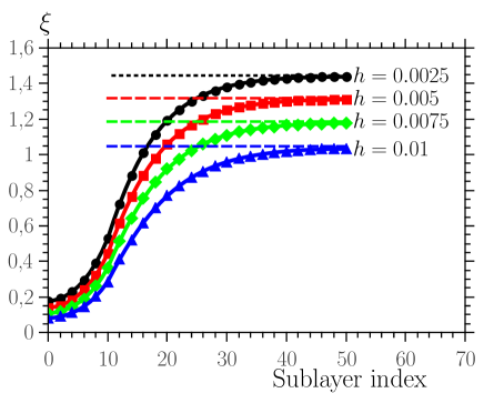
(b)

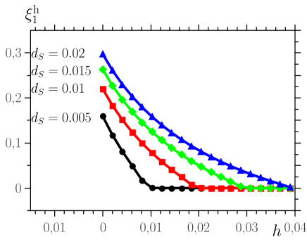
(c)

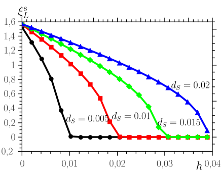
(d)

Figure 5: (a) System setup with inter-slab exchange interaction and applied field along the $z$ axis; (b) variation of the MP; (c) the deviation of the magnetic moment of the bottom HMS sub-layer $\xi_{1}^{\mathrm{h}}$ and (d) of the top SMS sub-layer $\xi_{L}^{\mathrm{s}}$ with the magnitude of the applied magnetic field with $\theta_{H}=0$. $\mathcal{N}_{h}=10$ and $\mathcal{N}_{s}=41$.

It is clear that the external field competes with the anisotropy and tends to align all the magnetic moments of the system parallel to its direction. Indeed, with enough layers in the SMS slab, $\xi_{L}^{{\rm s}}$ can be obtained from the Stoner–Wohlfarth equation

$$h\sin\left(\theta-\theta_{h}\right)-d_{s}\sin 2\theta=0.$$ (10)

In the specific case of $\theta_{h}=0$, we get $\theta=\arccos\left(h/2d_{s}\right)$, in agreement with the asymptotes (dashed lines) in Fig. 5(b). Indeed, Figs. 5(c) and 5(d) show that there is a critical value of the field, i.e. $h_{c}=2d_{s}$, at which all magnetic moments are aligned along the direction of the field, i.e. $\theta_{H}=0$. In this case, as the applied field is along the HMS anisotropy, $h_{c}$ is not affected by the latter. Hence, for a system with a sufficient number of layers in the SMS slab, $h_{c}$ will depend only on $d_{s}$. In general, however, $h_{c}$ should depend on $d_{h}$, $d_{s}$, and the applied field orientation. In cases where the system has less layers than the necessary number to attain the asymptotic value of $\xi_{1}^{{\rm h}}$ and $\xi_{L}^{\mathrm{s}}$ given by the SW equation (10), the magnitude of $h_{c}$ should decrease.

(a)

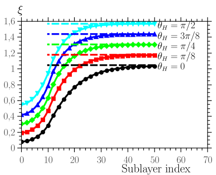
(b)

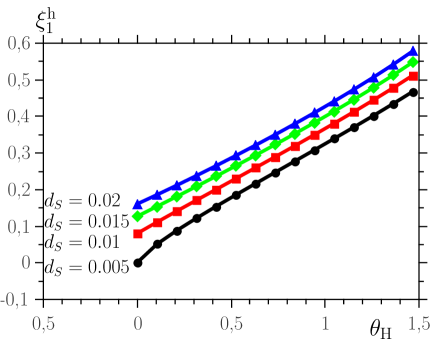
(c)

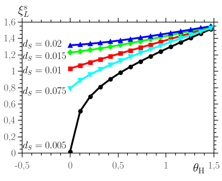
(d)

Figure 6: (a) System setup with inter-slab exchange interaction and applied field of varying direction; (b) variation of the MP; (c) deviation of the magnetic moment of the bottom HMS sub-layer $\xi_{1}^{\mathrm{h}}$ and (d) of the top SMS sub-layer $\xi_{L}^{\mathrm{s}}$ with the field direction $\theta_{H}$. $h=0.01$, $\mathcal{N}_{h}=10$ and $\mathcal{N}_{s}=41$.

Fig. 6 shows the same plots for a variable field orientation and the SMS intra-plane anisotropy $d_{{\rm s}}$, for $h=0.01$ and $\lambda_{\mathrm{EI}}=1.44$. We see that as the field is turned towards the SMS easy axis, the MP obviously shifts upwards with no noticeable change in shape, reaching a deviation at the top sub-layer that is again given by the numerical solution of the SW equation (Fig. 6(b) - dashed lines). Figs. 6(c) and 6(d) suggest that beyond a given $\theta_{H}$ the increase in the deviation is almost linear with a slope that depends on the anisotropy $d_{s}$. This implies a constant rate of change of $\xi_{1}^{{\rm h}}$ as it is mainly affected by $d_{h}$ (constant here), whereas the rate of change of $\xi_{L}^{{\rm s}}$ varies with $d_{s}$.

IV.2 Effect of inter-slab coupling

Now, we investigate the effect of the inter-slab coupling, considering successively EI, DDI, and DMI. In the end we compare their effects on the magnetization profile.

IV.2.1 Exchange interaction

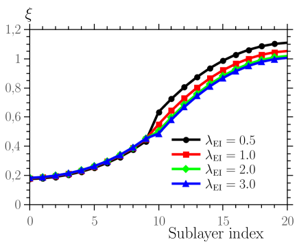
(a)

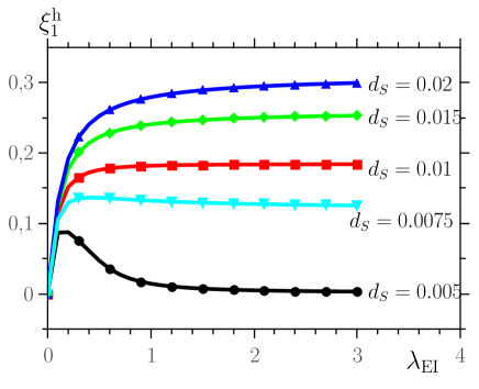
(b)

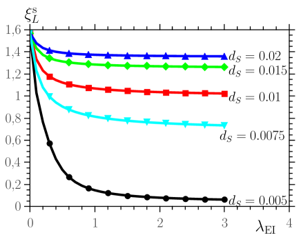
(c)

Figure 7: (a) Variation of MP and (b) deviation of the magnetic moment of the bottom HMS sub-layer $\xi_{1}^{\mathrm{h}}$ and (c) of the top SMS sub-layer $\xi_{L}^{\mathrm{s}}$ with the inter-slab EI $\lambda_{\mathrm{EI}}$. $\mathcal{N}_{h}=10$ and $\mathcal{N}_{s}=11$.

The results in Fig. 7(a) show that due to the strong anisotropy of the HMS slab, varying the inter-slab exchange coupling only affects the sub-layers in the SMS slab that starts here at $n=11$. On the other hand, the inter-slab exchange coupling competes with the intra-slab exchange coupling $J_{s}$ and anisotropy $D_{s}$ of the SMS slab. Thus the weaker $\lambda_{\mathrm{EI}}$ the stronger is the deviation.

Figs. 7(b) and 7(c) show the deviation $\xi_{1}^{{\rm h}}$ and $\xi_{L}^{{\rm s}}$ as functions of $\lambda_{\mathrm{EI}}$, respectively. As it could be expected, with increasing EI we achieve higher $\xi_{1}^{{\rm h}}$ and lower $\xi_{L}^{{\rm s}}$ deviations. As we effectively increase the rigidity of the interface, the HMS deviation at the interface thereby increases, whereas that of the SMS decreases. This change in deviation is then conveyed through all the sub-layers by means of the intra-layer EI, leading to the observed changes in $\xi_{1}^{{\rm h}}$ and $\xi_{L}^{{\rm s}}$. For low values of $d_{s}$, the $\xi_{1}^{{\rm h}}$ increase is much slower than the $\xi_{L}^{{\rm s}}$ decrease. However, as $d_{s}$ approaches $d_{h}=0.02$, the two become comparable as the two systems are close to being identical.

IV.2.2 Dipolar Interaction

In the present work we consider the system setup where the dipolar coupling is assumed to induce a ferromagnetic coupling between the two magnetic slabs.

(a)

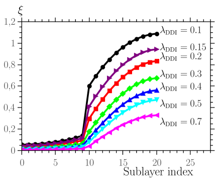
(b)

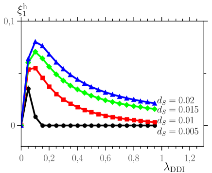
(c)

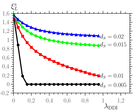
(d)

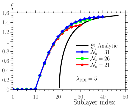
(e)

Figure 8: (a) System setup for a system with inter-slab dipolar interaction with a dipolar vector parallel to the HMS anisotropy; (b) variation of MP; (c) deviation of the magnetic moment of the bottom HMS sub-layer $\xi_{1}^{\mathrm{h}}$ and (d) of the top SMS sub-layer $\xi_{L}^{\mathrm{s}}$ with the inter-slab DDI $\lambda_{\mathrm{DDI}}$. (e) Comparison between RI analytical expressions and strong DDI numerical calculations. $\mathcal{N}_{h}=10$ and $\mathcal{N}_{s}=11$.

In Fig. 8(b) are plotted the MP for different values of the DDI inter-slab coupling $\lambda_{\mathrm{DDI}}$. Apart from the obvious shift upwards as $\lambda_{\mathrm{DDI}}$ decreases, there is an abrupt change at the interface especially for small $\lambda_{\mathrm{DDI}}$, mainly due to the fact that the in-plane anisotropy $d_{s}$ has a stronger effect than DDI.

Figs. 8(c) and 8(d) show that the system tends towards an asymptote as $\lambda_{\mathrm{DDI}}$ increases. In our case, since the DDI vector is parallel to the HMS anisotropy (along the $z$ axis), a strong enough interaction aligns the magnetic moments at the interface (and all the magnetic moments in the HMS) in the direction $\theta=0$, thus driving the system into an effective RI state. As such, the asymptote can be found by calculating $\xi_{L}^{{\rm s}}$ using the analytical expressions (de Sousa et al., 2010), i.e. Eqs. (2) and (3). Indeed, Fig. 8(e), where the MP is plotted for different values of $\mathcal{N}_{s}$ with very strong DDI ($\lambda_{\mathrm{DDI}}\sim 5$), shows a perfect agreement. Furthermore, if we examine the analytic curve (black line) near $n=20$ we observe a regime where a slight variation in $\mathcal{N}_{\mathrm{s}}$ induces a large change in $\xi_{L}^{\mathrm{s}}$, indicating that $\mathcal{N}_{s}=10$ is approximately the critical length of the SMS chain. A similar regime starts to be seen for stronger values of DDI in Fig. 8(b). Then, if we take into account that this behavior is not observed for weak DDI, it suggests that the critical length of the chain increases with increasing DDI.

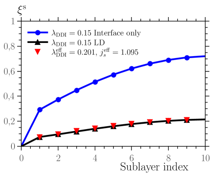
(a) $\mathcal{N}_{s}=10$

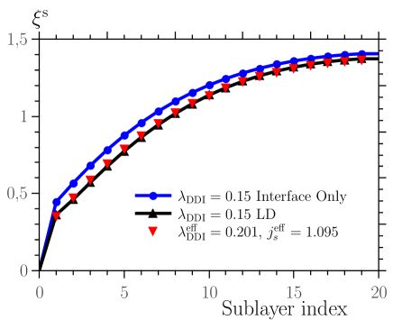
(b) $\mathcal{N}_{s}=20$

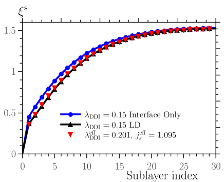
(c) $\mathcal{N}_{s}=30$

Figure 9: Comparison between different MP for a RI system with DDI at the interface only and with an effective value for both $\lambda_{\mathrm{DDI}}$ and $j_{s}$. $\lambda_{\mathrm{DDI}}=0.15$, $\lambda_{\mathrm{DDI}}^{\mathrm{eff}}=0.201$, $j_{s}^{\mathrm{eff}}=1.095$.

DDI is a long-ranged interaction that can penetrate through the SMS leading a priori to a coupling of the HMS interface with every SMS sub-layer, and vice-versa, with a strength $\xi\sim d^{-3}$ where $d$ is the distance between two magnetic moments. We also show in Fig. 8 that with $\lambda_{\mathrm{DDI}}$ at the interface with the bond $\mathbf{e}_{\mathrm{DDI}}$ along the $z$ axis, we can approximate the configuration of our system by a RI. Upon taking long distance interaction into account, the HMS interface will be coupled with every SMS sub-layer, but the SMS interface will only be coupled with the HMS at the interface, due to the latter being in a RI configuration. We call this a long distance (LD) configuration. Fig. 9 shows a comparison between the MP for $\lambda_{\mathrm{DDI}}=0.15$ only at the interface and LD configuration. The effect of the coupling penetration is a global decrease in the deviation of the magnetic moments of the SMS sub-layers. A similar behavior can be obtained with the effective couplings $\lambda_{\mathrm{DDI}}^{\mathrm{eff}}=0.201$ and $j_{s}^{\mathrm{eff}}=1.095$ with interaction only at the interface. This means that the effect of LD configuration is equivalent to that of an interaction which is limited to the interface, but with the re-normalized couplings $\lambda_{\mathrm{DDI}}^{\mathrm{eff}}$ and $j_{s}^{\mathrm{eff}}$. Figs. 9 (a)-(c) show that $\lambda_{\mathrm{DDI}}^{\mathrm{eff}}$ and $j_{s}^{\mathrm{eff}}$ do not change with the number of SMS sub-layers. However, Fig. 10 shows that they do depend on $\lambda_{\mathrm{DDI}}$.

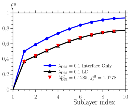
(a) $\lambda_{\mathrm{DDI}}=0.1$, $\lambda_{\mathrm{DDI}}^{\mathrm{eff}}=0.1285$, $j_{S}^{\mathrm{eff}}=1.0778$

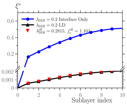
(b) $\lambda_{\mathrm{DDI}}=0.2$, $\lambda_{\mathrm{DDI}}^{\mathrm{eff}}=0.2815$, $j_{S}^{\mathrm{eff}}=1.104$

Figure 10: Comparison between MP for a RI system with DDI at the interface only, LD regime, and for the case with an effective values for $\lambda_{\mathrm{DDI}}$ and $j_{s}$ yielding the same MP as for the LD regime. $\mathcal{N}_{s}=10$.

IV.2.3 DM Interaction

As discussed in the introduction, it is relevant in the present study to investigate the effect of DMI on the dynamics of the MD, on the same footing as the (symmetrical) effective exchange coupling and anisotropic dipolar coupling. DM interaction may be induced by spin-orbit coupling between two ferromagnetic layers separated by a paramagnetic layer K. Xia, W. Zhang, M. Lu, and H. Zhai (1997); A. Crépieux and C. Lacroix (1998). It plays an important role in the presence of roughness and disorder at the interface of multi-layer systems. For a simple cubic lattice, on the (1 0 0) surface the DMI vector $\bm{D}$ lies in the layer plane and thus induces a perpendicular anisotropy. In the present work, we consider two situations where the DMI vector $\bm{D}$ lies either along the $x$ direction (thus in the $xy$ plane) or along the $z$ direction (i.e. normal to the $xy$ plane).

DM vector in the $x$ Direction

According to Eq. (7), the DMI tends to orientate the magnetic moments in such a way that they are normal to each other and perpendicular to the vector $\mathbf{D}$. Fig. 11(b) shows that with $\mathbf{D}$ along the $x$ axis, the HMS magnetic moments at the interface align along their easy axis $\mathbf{e}_{z}$, as it is perpendicular to the vector $\mathbf{D}$ and there are no other fields that could lead to a deviation from it. Therefore, all magnetic moments of the HMS slab will stick up along the direction $\theta=0$. On the other hand, the SMS magnetic moment at the interface, because it has to be perpendicular both to the HMS magnetic moment ($z$ axis) and the vector $\mathbf{D}$ ($x$ axis), lies in the $xy$ plane. However, in the SMS slab there is a competition between the DMI and the anisotropy $d_{s}$ in the $xy$ plane leading to a variable azimuthal angle $\varphi^{\mathrm{s}}$ as can be seen in Fig. 11 (c). With weaker DMI the anisotropy has a stronger effect and the SMS magnetization at the interface lies near the $x$ axis. As DMI increases the magnetization turns towards the $y$ axis as it has now to be perpendicular to the vector $\mathbf{D}$.

(a)

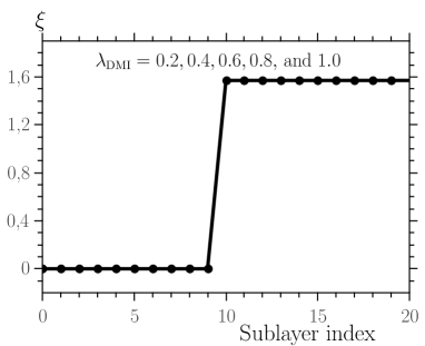
(b)

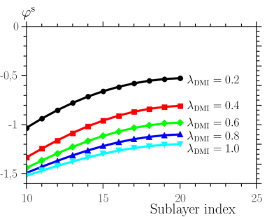
(c)

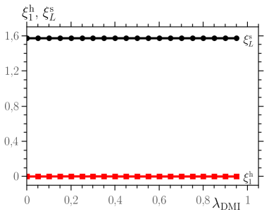
(d)

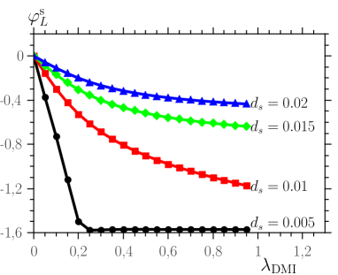
(e)

Figure 11: (a) System setup with inter-slab DMI interaction with a vector $\mathbf{D}$ perpendicular to the HMS easy axis; (b) variation of the polar MP ($\xi$); (c) azimuthal MP ($\varphi$), (d) the polar and (e) azimuthal deviations of the magnetic moments at the bottom HMS sub-layer $\xi_{1}^{\mathrm{h}}$ and the top SMS sub-layer $\xi_{L}^{\mathrm{s}}$ with the inter-slab DMI $\lambda_{\mathrm{DDI}}$, for various values of $d_{s}$.

In Fig. 11(d) we see that the HMS magnetization stays along the $z$ axis ($\xi_{1}^{\mathrm{h}}=0$) while that of the SMS slab remains in the $xy$ plane ($\xi_{L}^{\mathrm{s}}=\pi/2$) for values of $d_{s}=0.005,0.01,0.015$ and $0.02$. This means that the SMS magnetic moment at the interface is not affected by a varying SMS anisotropy in this setup. However, as is seen in Fig. 11(e) the $\varphi^{\mathrm{s}}$ dependence on the SMS-HMS coupling is affected by the anisotropy, exhibiting higher deviations for lower values of the anisotropy. Indeed, it is more favorable for the interaction to win the competition and drive the SMS interface magnetization onto the $y$ axis. For a strong enough interaction the SMS magnetization at the interface is pinned along the $y$ axis and the system can be modeled as a rigid magnet where the magnetization of the SMS varies in-plane with no out-of-plane component. In this situation, the top SMS magnetization can be calculated using Eq. (3) with now the angle variation $\xi_{L}$ referring to $\varphi_{L}^{\mathrm{s}}$ instead, because $\xi^{\mathrm{s}}$ is fixed at $\pi/2$.

Fig. 12 shows the MP similar to the one shown in Figs. 11 (b) and (c), but in this case we force the HMS magnetic moments to have a deviation $\xi^{\mathrm{h}}=\pi$, opposite to that of Fig. 11 (b), and we let the system evolve. This causes the orientation of the SMS magnetic moments to switch as well, thus demonstrating that for a system with this specific setup, it can be used as a “magnetic switch” since switching only the magnetic moment of the HMS slab induces a switching of the SMS magnetic moment. This is also true the other way round as is the case in exchange-spring systems where one attempts to achieve the reversal of the hard layer by smaller DC fields upon acting on the soft layer.

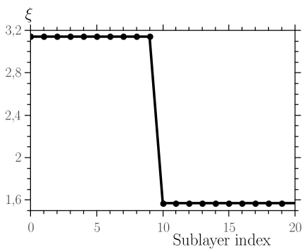
(a)

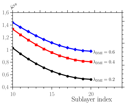
(b)

Figure 12: Magnetic “switch” behavior in the (a) out-of-plane ($\xi$) and (b) in-plane ($\varphi$) directions of the system with DMI at the interface and vector $\mathbf{D}$ along the $x$ axis. $\mathcal{N}_{h}=10$ and $\mathcal{N}_{s}=11$.

DM vector in the z Direction

Similarly to the previous case, the DMI will align the magnetic moment of one of the layers at the interface along the anisotropy axis of the corresponding slab, whereby its magnetization will not vary with the interaction. In the present case of $\bm{D}\parallel\bm{e}_{z}$, however, it is the SMS magnetic moment that remains constant because its anisotropy axis is normal to the vector $\mathbf{D}$. On the other hand, the HMS (net) magnetic moment becomes pinned in the $yz$ plane, implying that the angles $\varphi$ for both layers will remain constant and equal to $\varphi^{\mathrm{h}}=\pi/2$ and $\varphi^{\mathrm{s}}=0$. As such, the deviation at the interface for the HMS slab will vary according to the competition between the HMS anisotropy and the DMI, see Fig. 13(b). Hence, changes in the SMS anisotropy will not affect the MP of the system. Indeed, calculations of the $\xi_{1}^{h}$ and $\xi^{s}_{L}$ for various values of $d_{s}$ were performed and the same results, shown in Fig. 13(c), were obtained for all of them, thus confirming that the system is not affected by varying the value of the SMS anisotropy.

(a)

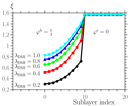
(b)

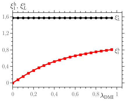
(c)

Figure 13: (a) System setup with inter-slab DMI interaction with a vector $\mathbf{D}$ parallel to the HMS anisotropy; (b) variation of the MP; (c) deviations of the magnetic moments at the bottom HMS sub-layer $\xi_{1}^{\mathrm{h}}$ and the top SMS sub-layer $\xi_{L}^{\mathrm{s}}$ with the inter-slab DMI $\lambda_{\mathrm{DDI}}$. $\mathcal{N}_{h}=10$ and $\mathcal{N}_{s}=11$.

For larger values of DMI the system can be viewed as an “inverted” rigid magnet, where the SMS and the HMS (net) magnetic moments at the interface are pinned in-plane. The out-of-plane variation of the HMS magnetic moment results from the competition between the HMS intra-slab exchange interaction and anisotropy. In this situation, the variation in the HMS magnetization can be calculated by using Eq. (3), upon substituting $d_{h}$ for $d_{s}$.

IV.2.4 Comparison between the inter-slab couplings

In Fig. 14 we present different magnetic profiles for typical values of the EI ($\lambda_{EI}=1.44$), DDI ($\lambda_{\mathrm{DDI}}/\lambda_{EI}\approx 10^{-2}$) and DMI ($\lambda_{\mathrm{DMI}}/\lambda_{EI}\approx 0.1$), as can be found in Refs. (Levy and Fert, 1981; A. Crépieux and C. Lacroix, 1998; de Sousa et al., 2010). Figs. 14 (left, right) present the MP in the polar ($\xi$) and azimuthal ($\varphi$) directions, respectively. In the polar MP the black curve with circles is the MP with only EI at the interface and serves as a reference. The red curve with squares is the MP obtained as we add DDI. Compared to the EI strength, the DDI is two orders of magnitude weaker and thereby its contribution to the alignment of the magnetic moments at the interface is very small. Nonetheless, it tends to align the interface along the $z$ axis and this effect propagates throughout all sub-layers by the in-plane exchange interaction, causing a global decrease in the MP. The dark blue curve (triangles up) represents the MP for DDI only. We see that the weak DDI is not sufficient to overcome the anisotropy of each sub-layer, leading only to a slight deviation near the interface but away from the latter each slab remains parallel to its easy axis. We observe an increased (induced) deviation in the SMS as compared to that of the HMS. This is due to the stronger anisotropy of the HMS enhanced by the DDI-induced anisotropy in the $z$ direction, making the out-of-plane direction more favorable at the interface than the in-plane direction. On the other hand, for the reasons given earlier, the DMI with its vector $\bm{D}$ along the $x$ axis, leads to a similar result with each slab aligned along its own easy axis even near the interface.

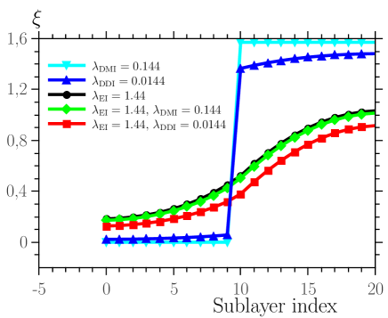
(a)

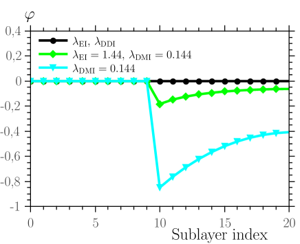
(b)

Figure 14: Effect of EI, DDI and DMI ($x$ direction) on the magnetic profile of a exchange spring, with $j=1.44$, $\lambda_{DDI}=0.0144$ and $\delta=0.144$. $\mathcal{N}_{h}=10$ and $\mathcal{N}_{s}=11$.

The MP in the azimuthal direction shown in Fig. 14 (right) compares the three inter-slab couplings. The EI and DDI are two interactions that do not induce an azimuthal rotation and the corresponding MP always lies in the same plane ($\varphi=0$). The green curve (with diamonds) is the MP obtained after adding DMI with its vector $\mathbf{D}$ in the $x$ direction. In Fig. 14 we see that the DMI induces a slight decrease in the deviation $\varphi^{\mathrm{s}}$ because the DMI tends to align the magnetic moments of the SMS slab along the $y$ axis, as is seen previously in Fig. 11(e). Even though the magnitude of this interaction was not high enough to overcome the anisotropy and internal exchange, it induced a deviation at the interface in the azimuthal direction. This deviation is, however, constrained by the EI at the interface and the anisotropies of the slabs. The light blue curve (triangles down) represents the MP for DMI with no exchange at the interface. As it could be expected, the magnetic moments of the HMS are all aligned along the $z$ axis (recall that $\mathbf{D}$ is along the $x$ axis), while those of the SMS slab are all in the $xy$ plane with a higher $\varphi$ deviation at the interface than in the previous case. This is obviously due to the fact that now the DMI competes only with the anisotropy of the SMS slab.

IV.2.5 Hysteresis loops

Here we present a succinct study of the hysteresis loop for different values of the interaction. It helps us to understand how the switching mechanism of the multi-layer system changes with the nature and strength of the inter-slab coupling. All the hysteresis curves presented are plots of the normalized magnetization $M_{z}/M_{s}$ versus reduced applied magnetic field $h$, along the HMS anisotropy axis ($z$ axis). $\mathcal{N}_{h}=12$ and $\mathcal{N}_{s}=16$. We start in a state of zero magnetization (i.e. the magnetic moments of all sub-layers are on the plane with no applied field) and iterate the LLE (5) until we reach the state of minimal energy. Next, we increase the applied field slightly and wait for the system to reach the new equilibrium state. We keep increasing the applied field until we reach saturation of the magnetization. Then, we ramp the field down and up again thus closing the hysteresis loop. Obviously, for each value of $h$, we wait until the state of minimal energy is reached.

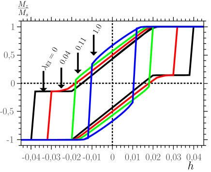
(a)

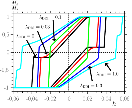
(b)

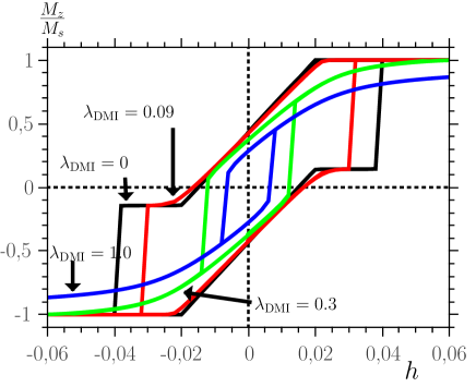
(c)

Figure 15: (a) Effect of EI, (b) of DDI, and (c) of DMI (along the $z$ axis) at the HMS-SMS interface on the hysteresis cycle and switching mechanisms of the HMS/SMS-SI multi-layer systems with $\mathcal{N}_{h}=12$ and $\mathcal{N}_{s}=16$.

Figure 15 (a) shows hysteresis cycles for different values of EI. Let us denote by $h_{s}^{c}$ the SMS switching field, by $h_{h}^{c}$ the HMS switching field, and by $h_{\mathrm{sat}}$ the saturation field of the whole multi-layer system. With no interaction ($\lambda_{\mathrm{EI}}=0$) and for $h=0$ the equilibrium state is that where the magnetic moments (of HMS and SMS) are oriented along their respective easy axes, i.e. $\theta_{k}=0$ and $\theta_{i}=\pi/2$ for all $k\in\mathrm{HMS},i\in\mathrm{SMS}$. The net magnetization of the system is that given by the HMS net magnetic moment projected on the $z$ axis. When $h$ is increased the magnetic moments of the SMS start to rotate towards the applied field in a reversible process until the system reaches saturation ($\theta_{k}=\theta_{i}=0$ for all $k,i$) at $h=h_{\mathrm{sat}}$. As we ramp down the field across zero until it reaches the SMS anisotropy field ($h_{s}^{c}=2d_{s}=0.02$), the SMS magnetic moments switch towards the field direction $\theta_{i}=\pi$ for all $i\in\mathrm{SMS}$. Further increase of the applied field (in the opposite direction) induces a slight reversible deviation of the HMS magnetization. In Fig. 15 (a) this corresponds to the plateau (on the $\lambda_{\mathrm{EI}}=0$ curve) from $h=-0.02$ to $h\simeq-0.04$, until $h$ reaches the HMS anisotropy field $h_{h}^{c}=h_{\mathrm{sat}}\simeq 2d_{h}=0.04$. At this value of the field, the HMS magnetic moments coherently switch from $\theta_{k}\approx 0$ to $\theta_{k}=\pi$, thus achieving negative saturation. Along the lower branch the system follows the same switching process from $\theta=\pi$ to $\theta=0$.

For nonzero but weak coupling, $\lambda_{\mathrm{EI}}=0.04$, the system follows the same behavior, but neither the HMS nor the SMS goes through a coherent rotation because of the inter-slab interaction. The SMS saturation field $h_{s}^{c}$ is now higher because its magnetization is stabilized by the interaction with the HMS. On the other hand, $h_{h}^{c}=h_{\mathrm{sat}}$ decreases because the molecular field of the already reversed SMS acts against the HMS anisotropy field. For stronger EI ($\lambda_{\mathrm{EI}}=0.11,1$) the plateau disappears completely ($h_{s}^{c}=h_{h}^{c}=h_{\mathrm{sat}}$), indicating that once the SMS magnetic moments reach a certain deviation, the EI induces a cascade effect in the HMS that causes the switching of the latter. The same observations of nonuniform magnetization switching leading to a smaller coercive field were made for magnetic recording exchange-spring media J. P. Wang, W. K. Shen, J. M. Bai, R. H. Victora, J. H. Judy, and W. L. Song (2005); A. Berger, N. Supper, Y. Ikeda, B. Lengsfield, A. Moser, and E. E. Fullerton (2008). Finally, an increase of the EI increases the remanent magnetization. The coercive field increases as long as $h_{\mathrm{sat}}>h_{s}^{c}$. As soon as the EI becomes strong enough to observe the cascade effect ($h_{\mathrm{sat}}=h_{s}^{c}$), the coercive field becomes a decreasing function of EI. Now, since the inter-layer exchange coupling decreases for an increasing spacer thickness, the coercive field passes by a minimum when the latter increases, again in agreement with what has been observed in Refs. J. P. Wang, W. K. Shen, J. M. Bai, R. H. Victora, J. H. Judy, and W. L. Song, 2005; A. Berger, N. Supper, Y. Ikeda, B. Lengsfield, A. Moser, and E. E. Fullerton, 2008.

Weak ($\lambda_{\mathrm{DDI}}=0,0.03$) or medium ($\lambda_{\mathrm{DDI}}=0.1,0.3$) DDI has a similar behavior to that of the EI, as can be seen in Fig. 15 (b). There is some difference, however, between the EI and DDI regarding the evolution of the hysteresis cycle as the inter-slab coupling is varied. While increasing EI decreases $h_{\mathrm{sat}}$, the DDI induces an increase of $h_{\mathrm{sat}}$ with increasing $\lambda_{\mathrm{DDI}}$. Indeed, DDI whose bond is along the $z$ axis induces an additional anisotropy at the interface along this axis and thereby tends to stabilize the magnetization in this direction. For $\lambda_{\mathrm{DDI}}=1.0$ the induced anisotropy field is stronger than the HMS anisotropy field. This implies that it is possible for the magnetic moments of the HMS that are far from the interface to switch before those at the interface. When the applied field becomes in excess of the induced-anisotropy field a complete switching is achieved. Finally, both the remanent magnetization and coercive field increase with DDI.

The effect of the DMI along the $z$ axis on the hysteresis cycle is shown in Fig. 15 (c). A similar behavior to those exhibited by EI and DDI for weak interaction ($\lambda_{\mathrm{DMI}}=0.09$) is observed. Again, we observe a progressive rotation of the SMS magnetization before the applied field becomes strong enough to induce a reversal of the HMS magnetization. As we discussed earlier, with no applied field the DMI along the $z$ axis induces a variation in the deviation of the magnetic moments of the HMS, while pinning the SMS (net) magnetic moment along the $x$ axis. The slight deviation induced in the magnetic moments of the HMS leads to a reduced HMS switching field $h_{h}^{c}=h_{\mathrm{sat}}$. Further increase of the interaction ($\lambda_{\mathrm{DMI}}=0.3,1$) induces again a cascade effect in the HMS that causes both slabs to switch in the same field ($h_{s}^{c}=h_{h}^{c}$). However, we have to note that unlike EI and DDI, the HMS/SMS switching field is not equal to $h_{\mathrm{sat}}$. This is again due to the deviation induced in the HMS magnetic moments by DMI. Both the remanent magnetization and the coercive field decrease with increasing DMI.

We can see that each kind of interaction induces a specific “single magnetic moment”-like behavior for strong coupling $\lambda$. A strong EI tends towards a system with no anisotropy, whereby the area of the loop tends to vanish, reaching saturation with very low applied fields in a switch-like behavior. DDI on the other hand tends to induce a square loop, typical of a very high uniaxial anisotropy with easy axis parallel to the applied field. Finally, the DMI tends to narrow the cycle and the magnetization follows the applied field, typical of a system with uniaxial anisotropy perpendicular to the field. Obviously, the perfect “single magnetic moment” behavior is never reached because the inter-slab interaction is present only at the interface and the deviation of the outer sub-layers is limited only by the intra-slab exchange interaction and the applied field.

V Conclusion

We have studied a magnetic multi-layer system composed of a hard magnetic slab with out-of-plane uniaxial anisotropy and a soft magnetic slab with in-plane uniaxial anisotropy, separated by a nonmagnetic spacer. We have considered three cases of inter-slab coupling, namely exchange, dipolar or Dzyaloshinski-Moriya interactions. The soft magnetic slab has been modeled as a stack of atomic (e.g. Fe) layers, while the hard magnetic slab has been modeled either as a macroscopic magnetic moment or as another stack of atomic (e.g. FePt) layers. Each atomic layer is modeled as a macroscopic magnetic moment representing its net magnetic moment, and is coupled to adjacent layers by exchange coupling.

We have investigated the effect of the external magnetic field, the in-plane or out-of-plane anisotropy, and the three interactions on the deviation angle (relative to the hard slab anisotropy easy axis). We have computed the magnetization profile through the whole multi-layer system. Our computing method consists in solving the set of (coupled) Landau-Lifshitz equations for the net magnetic moments of the layers. We first validate this method by comparing the corresponding results to the previously obtained analytical expressions for the case of exchange inter-slab coupling.

For the effect of the applied magnetic field, we found that with sufficient number of layers in the soft slab, the system behaves according to the Stoner–Wohlfarth regime and that there exists a critical field at which the whole system aligns along the applied field.

For exchange and dipolar interactions, there is an asymptotic value that depends on the anisotropy and the intra-layer exchange. For the dipolar interaction with a bond along the hard slab anisotropy, this asymptotic value is given by the analytical expression for rigid interface, where the hard slab is modeled as a single pinned magnetic moment, and only the variation in the soft slab is relevant. The dipolar interaction was next extended through the whole soft slab with a rigid interface. The ensuing effect on the magnetization profile of the soft slab has been recovered by an effective dipolar coupling at the interface only, upon re-scaling the intra-slab exchange coupling. The two corresponding effective coupling parameters depend on the initial dipolar interaction, but not on the number of SMS layers.

For the Dzyaloshinski-Moriya interaction, we found that the magnetic moments of one of the slabs are pinned in a given direction, whereas those of the remaining slab rotate in either the polar angle or the azimuthal angle, depending on the direction of the vector $\mathbf{D}$. Large values of the DM coupling lead to a system with rigid interface, with the magnetic moments at the interface being perpendicular to each other and to the vector $\mathbf{D}$. In addition, a switch-like mechanism can be achieved with this interaction. Indeed, an indirect reversal of the SMS magnetization can be achieved by directly forcing a reversal of the HMS magnetization with the help of a magnetic field. It is obviously also possible to obtain the desired effect for the exchange-spring system by achieving the reversal of HMS via the switching of the SMS magnetization with the help of a smaller magnetic field.

A comparison between the three interactions with typical orders of magnitude has been given. The exchange coupling shows the strongest effect, and when added, the dipolar and Dzyaloshinski-Moriya interactions induce a slight (but non negligible) deviation in either the polar or azimuthal magnetization profile.

Finally, hysteresis cycles for the three different interactions are computed. A typical exchange spring behavior, where the soft slab switches first, followed by the hard slab at a stronger field, is observed for weak interaction in all cases. Strong coupling causes both slabs to switch under the same field. Exchange and Dzyaloshinski-Moriya interactions tend to narrow the cycle, while the dipolar interaction leads to squared cycles. For application purposes such as magnetic recording using vertical exchange-spring media, the Dzyaloshinski-Moriya inter-layer coupling strongly reduces the coercive field while keeping high values of the anisotropy which thus ensure good thermal stability.

A work in progress consists in treating each atomic layer as a two-dimensional lattice with the aim to compute spin correlations as functions of the various energy parameters and to determine the spin-wave spectrum. In the near future, this zero-temperature study will be extended to finite temperature with the aim to investigate thermal effects with special emphasis on the calculation of activation rates of such multi-layer systems and thereby assess their thermal stability.

References

- E. F. Kneller and R. H. Hawig (1991) E. F. Kneller and R. H. Hawig, IEEE Trans. Magn. 27, 3588 (1991).
- R. H. Victora, X. Shen (2005) R. H. Victora, X. Shen, IEEE Trans. Magn. 41, 537 (2005).
- D. Suess, T. Schrefl, R. Dittrich, M. Kirschner, F. Dorfbauer, G. Hrkac, J. Fidler (2005) D. Suess, T. Schrefl, R. Dittrich, M. Kirschner, F. Dorfbauer, G. Hrkac, J. Fidler, J. Magn. Magn. Mater. 290, 551 (2005).
- K.B. Urquhart, B. Heinrich, J.F. Cochran, A.S. Arrott, and Myrtle (1988) K.B. Urquhart, B. Heinrich, J.F. Cochran, A.S. Arrott, and Myrtle, J. Appl. Phys. 64, 5334 (1988).
- B. Heinrich and J.F.C. Cochran (1993) B. Heinrich and J.F.C. Cochran, Adv. Phys 42, 523 (1993).
- B. Heinrich (1994) B. Heinrich, in Ultrathin magnetic structures II, edited by B. Heinrich and J. Bland (Springer-Verlag, Berlin, 1994), p. 195.
- Farle (1998) M. Farle, Rep. Prog. Phys. 61, 755 (1998).
- G. Woltersdorf and Ch. H. Back (2007) G. Woltersdorf and Ch. H. Back, Phys. Rev. Lett. 99, 227207 (2007).
- J.F. Cochran (1994) J.F. Cochran, in Ultrathin magnetic structures II, edited by B. Heinrich and J. Bland (Springer-Verlag, Berlin, 1994), p. 222.
- C. Mathieu et al. (1998) C. Mathieu et al., Phys. Rev. Lett. 81, 3968 (1998).
- E. Beaurepaire, J.-C. Merle, A. Daunois, and J.-Y. Bigot (1996) E. Beaurepaire, J.-C. Merle, A. Daunois, and J.-Y. Bigot, Phys. Rev. Lett. 76, 4250 (1996).
- B. Koopmans, M. van Kampen, J. T. Kohlhepp, and W. J. M. de Jonge (2000) B. Koopmans, M. van Kampen, J. T. Kohlhepp, and W. J. M. de Jonge, Phys. Rev. Lett. 85, 844 (2000).
- M. van Kampen, C. Jozsa, J. T. Kohlhepp, P. LeClair, W. J. M. de Jonge, and B. Koopmans (2002) M. van Kampen, C. Jozsa, J. T. Kohlhepp, P. LeClair, W. J. M. de Jonge, and B. Koopmans, Phys. Rev. Lett. 88, 227201 (2002).
- J. Stöer and H. C. Siegmann (2006) J. Stöer and H. C. Siegmann, Magnetism: from fundamentals to nanoscale dynamics (Springer, Berlin, 2006).
- P. Bruno (1995) P. Bruno, Phys. Rev. B 52, 411 (1995).
- A. Berger, N. Supper, Y. Ikeda, B. Lengsfield, A. Moser, and E. E. Fullerton (2008) A. Berger, N. Supper, Y. Ikeda, B. Lengsfield, A. Moser, and E. E. Fullerton, Appl. Phys. Lett. 93, 122502 (2008).
- J. P. Wang, W. K. Shen, J. M. Bai, R. H. Victora, J. H. Judy, and W. L. Song (2005) J. P. Wang, W. K. Shen, J. M. Bai, R. H. Victora, J. H. Judy, and W. L. Song, Appl. Phys. Lett. 86, 142504 (2005).
- D. Suess, T. Schrefl, S. Faehler, M. Kirschner, G. Hrkac, F. Dorfbauer, and J. Fidler (2005) D. Suess, T. Schrefl, S. Faehler, M. Kirschner, G. Hrkac, F. Dorfbauer, and J. Fidler, Appl. Phys. Lett. 87, 012504 (2005).
- D. Suess, T. Schrefl, M. Kirschner, G. Hrkac, F. Dorfbauer, O. Ertl, and J. Fidler (2005) D. Suess, T. Schrefl, M. Kirschner, G. Hrkac, F. Dorfbauer, O. Ertl, and J. Fidler, IEEE Trans. Magn. 41, 3166 (2005).
- K. C. Schuermann, J. D. Dutson, S. Z. Wu, S. D. Harkness, B. Valcu, H. J. Richter, R. W. Chantrell, and K. O’Grady (1993) K. C. Schuermann, J. D. Dutson, S. Z. Wu, S. D. Harkness, B. Valcu, H. J. Richter, R. W. Chantrell, and K. O’Grady, J. Appl. Phys. 99, 08Q904 (2006).
- E. W. Hill, S. L. Tomlinson, J.-P. Li (1993) E. W. Hill, S. L. Tomlinson, J.-P. Li, J. Appl. Phys. 73, 5978 (1993).
- Vargas and Altbir (2000) P. Vargas and D. Altbir, Phys. Rev. B 62, 6337 (2000).
- K. Xia, W. Zhang, M. Lu, and H. Zhai (1997) K. Xia, W. Zhang, M. Lu, and H. Zhai, Phys. Rev. B 55, 12561 (1997).
- B. Heinrich et al. (2003) B. Heinrich et al., Phys. Rev. Lett. 90, 187601 (2003).
- G. N. Kakazei, Yu. G. Pogorelov, M. D. Costa, V. O. Golub, J. B. Sousa, P. P. Freitas, S. Gardoso, and P. E. Wigen (1926) G. N. Kakazei, Yu. G. Pogorelov, M. D. Costa, V. O. Golub, J. B. Sousa, P. P. Freitas, S. Gardoso, and P. E. Wigen, Z. Phys. 38, 518 (1926).
- B. Skubic et al. (2006) B. Skubic et al., Phys. Rev. Lett. 96, 057205 (2006).
- M. Madami et al. (2008) M. Madami et al., J. Appl. Phys. 104, 063510 (2008).
- L. Sun et al. (2011) L. Sun et al., J. Appl. Phys. 109, 033913 (2011).
- C. Lacroix, B. Dieny, J. P. Gavigan, and D. Givord (1990) C. Lacroix, B. Dieny, J. P. Gavigan, and D. Givord, Thin solid films 193/194, 877 (1990).
- Y. Wang, P. M. Levy, and J. L. Fry (1990) Y. Wang, P. M. Levy, and J. L. Fry, Phys. Rev. Lett. 65, 2732 (1990).
- D. Altbir, M. Kiwi, R. Ramírez, and I. K. Schuller (1995) D. Altbir, M. Kiwi, R. Ramírez, and I. K. Schuller, J. Magn. Magn. Mater. 149, L246 (1995).
- D. M. Edwards, R. P. Erickson, J. Mathon, R. B. Muniz, and M. Villeret (1995) D. M. Edwards, R. P. Erickson, J. Mathon, R. B. Muniz, and M. Villeret, Mater. Sci. Eng. B 31, 25 (1995).
- I. Dzyaloshinsky (1958) I. Dzyaloshinsky, J. Phys. Chem. Solids 4, 241 (1958).
- T. Moriya (1960) T. Moriya, Phys. Rev. Lett. 4, 228 (1960).
- A. Crépieux and C. Lacroix (1998) A. Crépieux and C. Lacroix, J. Magn. Magn. Mater. 182, 341 (1998).
- T. Moriya (1960) T. Moriya, Phys. Rev. 120, 91 (1960).
- A. F. Franco, J. M. Martinez, J. L. Déjardin, and H. Kachkachi (2011) A. F. Franco, J. M. Martinez, J. L. Déjardin, and H. Kachkachi, Phys. Rev. B 84, 134423 (2011).
- de Sousa et al. (2010) N. de Sousa, A. Apolinario, F. Vernay, P. M. S. Monteiro, F. Albertini, F. Casoli, H. Kachkachi, and D. S. Schmool, Phys. Rev. B 82, 104433 (2010).
- Levy and Fert (1981) P. M. Levy and A. Fert, Phys. Rev. B 23, 4667 (1981).