Looking for the rainbow on exoplanets covered by liquid and icy water clouds

Abstract

Aims. Looking for the primary rainbow in starlight that is reflected by exoplanets appears to be a promising method to search for liquid water clouds in exoplanetary atmospheres. Ice water clouds, that consist of water crystals instead of water droplets, could potentially mask the rainbow feature in the planetary signal by covering liquid water clouds. Here, we investigate the strength of the rainbow feature for exoplanets that have liquid and icy water clouds in their atmosphere, and calculate the rainbow feature for a realistic cloud coverage of Earth.

Methods. We calculate flux and polarization signals of starlight that is reflected by horizontally and vertically inhomogeneous Earth–like exoplanets, covered by patchy clouds consisting of liquid water droplets or water ice crystals. The planetary surfaces are black.

Results. On a planet with a significant coverage of liquid water clouds only, the total flux signal shows a weak rainbow feature. Any coverage of the liquid water clouds by ice clouds, however, dampens the rainbow feature in the total flux, and thus the discovery of liquid water in the atmosphere. On the other hand, detecting the primary rainbow in the polarization signal of exoplanets appears to be a powerful tool for detecting liquid water in exoplanetary atmospheres, even when these clouds are partially covered by ice clouds. In particular, liquid water clouds covering as little as 10%–20% of the planetary surface, with more than half of these covered by ice clouds, still create a polarized rainbow feature in the planetary signal. Indeed, calculations of flux and polarization signals of an exoplanet with a realistic Earth–like cloud coverage, show a strong polarized rainbow feature.

1 Introduction

The discovery of the first exoplanet orbiting a main sequence star almost two decades ago (Mayor & Queloz 1995) inaugurated a new era in astronomy. As of today, more than 700 exoplanets have been detected (source: The extrasolar planets encyclopeadia). Telescope instruments and satellite missions, like for example COROT (COnvection, ROtation & planetary Transits) (Baglin et al. 2006), NASA’s Kepler mission (Koch et al. 1998), HARPS (High Accuracy Radial Velocity Planet Searcher) (e.g. Pepe et al. 2004), Super–WASP (Deming et al. 2012), and, in the near future, GPI (Gemini Planet Imager) (Macintosh et al. 2008) on the Gemini observatory (first on the telescope on the southern hemisphere) and SPHERE (Spectro–Polarimetric High–Contrast Exoplanet Research) (e.g. Dohlen et al. 2008; Roelfsema et al. 2011) on ESO’s Very Large Telescope (VLT), to name a few, will rapidly increase the number of detected exoplanets.

The detection methods used and the accuracy of our instruments result in most of the exoplanets detected up to today being giants, even though in recent years the lower mass limit of our detections has been pushed down allowing for the detection of more than 30 super–Earth planets. With an increasing possibility for the detection of the first Earth–like planets in the next decade, an important factor to consider is how ready our models will be to interpret the observations.

An important factor that needs to be taken into account for future efforts to detect signatures of life on other planets is the possible inhomogeneity of the planetary surface and atmosphere (Tinetti et al. 2006, and references therein). The existence of continents, oceans and variable atmospheric patterns (cloud patches etc), as well as their distributions across the planetary surface can have a large impact on the observed signal. For this reason, the models that we use to interpret the observations should be able to handle inhomogeneous planets.

There exist a number of models that deal with the brightness of inhomogeneous exoplanets (Ford et al. 2001; Tinetti 2006; Montañés-Rodríguez et al. 2006; Pallé et al. 2008, to name a few). All of the models show the importance of planetary inhomogeneity and temporal variability on the modelled planetary signal. The pioneering work of Ford et al. (2001) as well as later studies (e.g. Oakley & Cash 2009), show a clear diurnal variability of the modelled Earth–as–an–exoplanet signal due to areas of different albedo passing in and out of the observational field of view.

Among the factors that influence the planetary signal, clouds have a prominent role. Observations of earthshine for example, have shown that clouds can induce a considerable daily variation in the planetary signal. The amount of variability observed differs slightly among the observations ($\sim 10$% for Pallé et al. (2004), $\sim 5$% for Goode et al. (2001) and a few percent for Cowan et al. (2009)). Cloud coverage and variability can also influence to a large degree the interpretation of the observations. Oakley & Cash (2009) for example find that mapping the planetary surface is only possible for cloud coverages smaller than the mean Earth one. Even in the case of giant planets or dwarf stars, clouds play a crucial role in defining the atmospheric thermal profile and eventually spectra (Marley et al. 2010).

At present, the characterization of exoplanets is mainly done using planetary transits with instruments on e.g. the Hubble and Spitzer Space Telescopes (see e.g. Ehrenreich et al. 2007; Deming et al. 2011; Tinetti & Griffith 2010), and for some planets, even with ground–based instrumentation (see e.g. Snellen et al. 2010; Brogi et al. 2012; de Mooij et al. 2012). With the transit method though, during the primary transit, the observed starlight has only penetrated the upper layers of the planetary atmosphere. Cloud layers at lower altitudes could for example block out the signal from lower atmospheric layers or a possible planetary surface. Even with the help of secondary transits, the characterisation of Earth–like exoplanets in the habitable zone of a solar–type star would not be possible, since these planets would yield too weak a signal (Kaltenegger & Traub 2009). Direct observations of reflected starlight from the planet could solve this problem, since then information from the lower atmospheric layers and surface could survive in the observed planetary signal. The combination in these cases of flux and polarization observations could provide us with a crucial tool to break any possible retrieval degeneracies (for example, such as between optical thicknesses and single scattering albedo’s or cloud particle sizes) that flux only measurements may present. A first detection of an exoplanet using polarimetry was claimed by Berdyugina et al. (2008). Subsequent polarization observations by Wiktorowicz (2009) could, however, not confirm this detection. In 2011 Berdyugina et al. (2011) presented another detection of the same planet at shorter wavelengths, which still awaits confirmation by follow–up observations. Telescope instruments like GPI (Macintosh et al. 2008) and SPHERE (e.g. Dohlen et al. 2008; Roelfsema et al. 2011), which have polarimetric arms that have been optimized for exoplanet detection, are expected to detect and characterize exoplanets with polarimetry in the near future.

The power of polarization in studying planetary atmospheres and surfaces has been shown multiple times in the past through observations of Solar System planets (including Earth itself)(see for example Hansen & Hovenier 1974; Hansen & Travis 1974; Mishchenko 1990; Tomasko et al. 2009), as well as by modeling of solar system planets or giant and Earth–like exoplanets (e. g.  Stam 2003; Stam et al. 2004; Saar & Seager 2003; Seager et al. 2000; Stam 2008; Karalidi et al. 2011). Polarization provides us with a unique tool for the detection of liquid water on a planetary atmosphere and surface. Williams & Gaidos (2008) e.g. use polarization to detect the glint of starlight reflected on liquid surfaces (oceans) of exoplanets and Zugger et al. (2010, 2011) conclude that the existence of an atmosphere as thick as Earth’s would hide any polarization signature of the underlying oceans. Probably the most interesting feature to look for in the polarization signal of exoplanets is the rainbow.

The rainbow is a direct indication of the presence of liquid water droplets in a planetary atmosphere (see e.g. Bailey 2007; Karalidi et al. 2011). Its angular position depends strongly on the refractive index of the scattering particles and slightly on their effective radius (see Karalidi et al. 2011, and references therein). Its existence, most pronounced in polarization observations, can be masked by the existence of ice clouds (Goloub et al. 2000). The latter are often located above thick liquid water clouds and can dominate the appearance of the reflected polarization signal for ice cloud optical thicknesses larger than 2 (Goloub et al. 2000).

In Karalidi et al. (2011), we calculated flux and polarization signals for horizontally homogeneous model planets that were covered by liquid water clouds. The polarization signals of these planets clearly contained the signature of the rainbow. The polarization signals of the quasi horizontally inhomogeneous planets (where weighted sums of horizontally homogeneous planets are used to approximate the signal of a horizontally inhomogeneous planet) as presented by Stam (2008) also show the signature of the rainbow. However, to confirm that realistically horizontally inhomogeneous planets, with patchy liquid water clouds, and with patchy liquid water clouds covered by patchy ice clouds, also show the signature of the rainbow, the algorithm for horizontally inhomogeneous planets as described in Karalidi & Stam (accepted) is required. In this paper we will do exactly that: using the algorithm of Karalidi & Stam (accepted) to look for the rainbow on horizontally inhomogeneous planets, that are covered by different amounts of liquid and icy water clouds.

This paper is organized as follows. In Sect. 2, we give a short description of polarized light and our radiative transfer algorithm, and present the model planets and the clouds we use. In Sect. 3, we investigate the influence of the liquid water cloud coverage on the strength of the rainbow feature of a planet in flux and polarization. In Sects. 4 and 5 we investigate the influence of different cloud layers, respectively with different droplet sizes and with different thermodynamic phases (liquid or ice), on the strength of the rainbow feature. An interesting test case for the detection of a rainbow feature is of course the Earth itself. In Sect. 6, we use realistic cloud coverage, optical thickness and thermodynamic phase data from the MODIS satellite instrument to investigate whether the rainbow feature of water clouds would appear in the disk integrated sunlight that is reflected by the Earth. Finally, in Sect. 7, we present a summary of our results and our conclusions.

2 Calculating flux and polarization signals

2.1 Defining flux and polarization

We describe starlight that is reflected by a planet by a flux vector $\pi\@vec{F}$, as follows

$$\pi\@vec{F}=\pi\left[\begin{array}[]{c}F\\ Q\\ U\\ V\end{array}\right],$$ (1)

where parameter $\pi F$ is the total flux, parameters $\pi Q$ and $\pi U$ describe the linearly polarized flux and parameter $\pi V$ the circularly polarized flux (see e.g. Hansen & Travis 1974; Hovenier et al. 2004; Stam 2008). All four parameters depend on the wavelength $\lambda$, and their dimensions are W m^-2m^-1. Parameters $\pi Q$ and $\pi U$ are defined with respect to a reference plane, and as such we chose here the planetary scattering plane, i.e. the plane through the center of the star, the planet and the observer. Parameter $\pi V$ is usually small (Hansen & Travis 1974), and we will ignore it in our numerical simulations. Ignoring $\pi V$ will not introduce significant errors in our calculated total and polarized fluxes (Stam & Hovenier 2005).

The linearly polarized flux, $\pi F_{\mathrm{P}}$ of flux vector $\pi\@vec{F}$ is independent of the choice of the reference plane and is given by

$$\pi F_{\rm P}=\pi\sqrt{Q^{2}+U^{2}},$$ (2)

while the degree of (linear) polarization $P$ is defined as the ratio of the linearly polarized flux to the total flux, as follows

$$P=\frac{F_{\rm P}}{F}=\frac{\sqrt{Q^{2}+U^{2}}}{F}.$$ (3)

For a planet that is mirror–symmetric with respect to the planetary scattering plane, parameter $U$ will be zero. In this case we use the signed degree of linear polarization $P_{\mathrm{s}}=-Q/F$, which includes the direction of polarization: if $P_{\mathrm{s}}>0$ ($P_{\mathrm{s}}<0$), the light is polarized perpendicular (parallel) to the plane containing the incident and scattered beams of light. A planet with patchy clouds will usually not be mirror–symmetric with respect to the planetary scattering plane, and hence $U$ will usually not equal zero.

The flux vector $\pi\@vec{F}$ of stellar light that has been reflected by a spherical planet with radius $r$ at a distance $d$ from the observer ($d\gg r$) is given by (Stam et al. 2006)

$$\pi\@vec{F}(\lambda,\alpha)=\frac{1}{4}\frac{r^{2}}{d^{2}}\@vec{S}(\lambda,\alpha)\pi\@vec{F}_{0}(\lambda).$$ (4)

Here, $\lambda$ is the wavelength of the light and $\alpha$ the planetary phase angle, i. e. the angle between the star and the observer as seen from the center of the planet. Furthermore, $\@vec{S}$ is the 4$\times$4 planetary scattering matrix (Stam et al. 2006) with elements $a_{ij}$ and $\pi\@vec{F}_{0}$ is the flux vector of the incident stellar light. For a solar type star, the stellar flux can be considered to be unpolarized when integrated over the stellar disk (Kemp et al. 1987).

We assume that the ratio of the planetary radius $r$ and the distance to the observer $d$ is equal to one, and that the incident stellar flux $\pi F_{0}$ is equal to $1$ W m^-2 m^-1. The hence normalised flux $\pi F_{\mathrm{n}}$ that is reflected by a planet is thus given by

$$\pi F_{\mathrm{n}}(\lambda,\alpha)=\frac{1}{4}a_{11}(\lambda,\alpha)$$ (5)

(see Stam 2008; Karalidi et al. 2011), and corresponds to the planet’s geometric albedo $A_{\mathrm{G}}$ when $\alpha=0^{\circ}$. The corresponding normalized polarized flux is given by

$$\pi F_{\mathrm{n,P}}(\lambda,\alpha)=\frac{1}{4}\sqrt{a_{21}(\lambda,\alpha)^{2}+a_{31}(\lambda,\alpha)^{2}},$$ (6)

with $a_{21}$ and $a_{31}$ elements of the planetary scattering matrix. Our normalized fluxes $\pi F_{\mathrm{n}}$ can straightforwardly be scaled for any given planetary system using Eq. 4 and inserting the appropriate values for $r$, $d$ and $\pi F_{0}$. The degree of polarization $P$ is independent of $r$, $d$ and $\pi F_{0}$, and will thus not require any scaling.

2.2 The radiative transfer calculations

The code that we use to calculate the total and polarized fluxes of starlight that is reflected by a model planet fully includes single and multiple scattering, and polarization. It is based on the same efficient adding-doubling algorithm (de Haan et al. 1987) used by Stam et al. (2006); Stam (2008). To calculate flux and polarization signals of horizontally inhomogeneous planets, we divide a model planet in pixels with a size such that we can assume that the surface and atmospheric layers are locally plane parallel and horizontally homogeneous. We then use the code for horizontally inhomogeneous planets, as presented in Karalidi & Stam (accepted): the contribution of every illuminated pixel that is visible to the observer to the planet’s total and polarized flux are calculated separately, the polarized fluxes are rotated to the common reference plane, and then all fluxes are summed up to get the disk–integrated planetary total and polarized fluxes. From these fluxes, the disk–integrated degree of linear polarization $P$ is derived (Eq. 3).

As before (Karalidi & Stam accepted), we divide our model planets in plane–parallel, horizontally homogeneous (but vertically inhomogeneous) pixels of $2^{\circ}\times 2^{\circ}$. Our pixels are large enough to be able to ignore adjacency effects, i.e. light that is scattered and/or reflected within more than one pixel (e.g. light that is reflected by clouds in one pixel towards the surface of another pixel). These effects, that make the fluxes emerging from a given type of pixel dependent on the properties of the surrounding pixels, show up for higher spatial resolutions, for example, with pixels that are smaller than about 1$\times$1 km² (Marshak et al. 2008).

2.3 The model planets

All model planets have a vertical inhomogeneous atmosphere on top of a black surface. The assumption of a black surface is a very good approximation for an ocean surface (without the glint), which covers most of the Earth’s surface. We’ll discuss the effects of brighter surfaces on our results where necessary. All model atmospheres have a pressure and temperature profile representative for a mid-latitude atmosphere (McClatchey et al. 1972) (see Fig. 1). We divide each model atmosphere in the same 16 layers. The total gaseous (Rayleigh) scattering optical thickness of the atmosphere is 0.097 at $\lambda=0.550\leavevmode\nobreak\ \mu$m and 0.016 at $\lambda=0.865\leavevmode\nobreak\ \mu$m. We do not include gaseous absorption, which is a good assumption at the wavelengths of our interest.

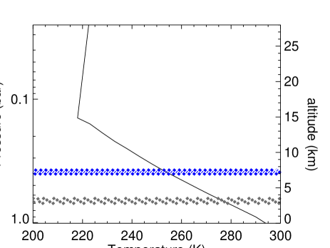
Figure 1: The atmospheric pressure and altitude as functions of the temperature for the model planets. The liquid water clouds are located below 4 km (for example in between 3 km and 4 km as in the gray, dotted area), and the ice clouds between 7 km and 8 km (blue, dashed–dotted area).

The flux and polarization signals of our model planets are fairly insensitive to the pressure and temperature profiles, but they are sensitive to the horizontal and vertical distribution of the clouds, and to the microphysical properties of the cloud particles. We will use two types of clouds: the first type consisting of liquid water droplets, and the second type consisting of water ice particles. The details of these particles will be discussed in Sect. 2.4. The liquid water clouds will be located below an altitude of 4 km (i.e. at pressures lower than 0.628 bars, which corresponds to temperatures higher than 273 K) and the ice clouds above that altitude.

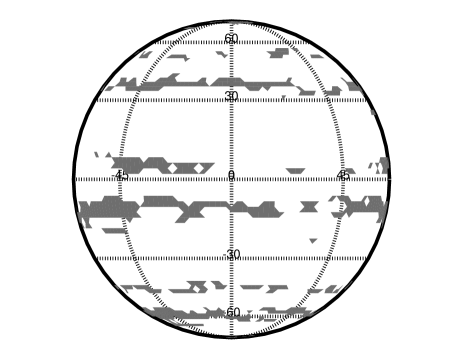
Figure 2: A sample map of our model planets. Here, the planetary atmosphere contains a single layer with clouds that cover $\sim$ 25% of the planet (the dark regions are the clouds).

We create our cloud maps by using an ISCCP yearly cloud map which we filter according to the clouds’ optical thicknesses. Figure 2 shows a sample map for a model planet with a single cloud layer that covers $\sim$25% of the planet. As shown in Karalidi & Stam (accepted), the precise location of clouds can influence in particular the polarized phase function of a planet (i.e. the degree of polarization of the reflected starlight as a function of the planetary phase angle). To avoid changes in $\pi F_{\mathrm{n,P}}$ and $P$ due to the location of clouds when the coverage increases, we increase the cloud coverage of a planet by letting existing clouds grow in size. Cloudy regions thus remain cloudy, while surface patches are getting cloudy.

2.4 The cloud particles

The liquid water cloud particles are spherical, with the standard size distribution given by (Hansen & Travis 1974)

$$n(r)=Cr^{(1-3v_{\rm eff})/v_{\rm eff}}e^{-r/r_{\rm eff}v_{\rm eff}},$$ (7)

with $n(r)\mathrm{d}r$ the number of particles per unit volume with radius between $r$ and $r+\mathrm{d}r$, $C$ a constant of normalization, $r_{\mathrm{eff}}$ the effective radius and $v_{\mathrm{eff}}$ the effective variance of the distribution. Terrestrial liquid water clouds are in general composed of droplets with radii ranging from $\sim 5\leavevmode\nobreak\ \mu$m to $\sim 30\leavevmode\nobreak\ \mu$m (Han et al. 1994). We use either small droplets (type A), with $r_{\mathrm{eff}}=2.0$ $\mu$m and $v_{\mathrm{eff}}=0.1$, or larger droplets (type B) with $r_{\mathrm{eff}}=6.0$ $\mu$m and $v_{\mathrm{eff}}=0.4$ (see also Karalidi et al. 2011). The latter are similar to those used by van Diedenhoven et al. (2007) as average values for terrestrial water clouds. We use a wavelength independent refractive index of 1.335+0.00001$i$ (see Karalidi et al. 2011, and references therein). For a given wavelength, and values of $r_{\mathrm{eff}}$ and $v_{\mathrm{eff}}$, we calculate the extinction cross–section, single scattering albedo and the single scattering matrix using Mie–theory (de Rooij & van der Stap 1984) and normalized according to Eq. 2.5 of Hansen & Travis (1974).

Ice crystals in nature present a large variety of shapes, depending on the temperature and humidity conditions during their growth (Hess 1998). Even though the variety of shapes is large, Magono & Lee (1966) showed that only a small number of classes suffice for the categorization of most natural ice crystals. Until recently most researchers used perfect hexagonal columns and plates in order to model the light scattered by natural ice crystals, including halo phenomena. However, when these particles are oriented, they give rise to halos, which are rarely observed (Macke et al. 1996; Hess 1998). For this reason a number of models were created to model the signal of ice crystals without halo phenomena (Hess & Wiegner 1994; Macke et al. 1996; Hess 1998). In this paper we use an updated version of the model crystals of Hess (1998). Finally, we should mention that the sizes of most atmospheric ice crystals are considerably larger than the visible wavelengths we will use in this paper (Macke et al. 1996). In particular, the crystals we use in this paper range in size from $\sim$6 $\mu$m up to $\sim$2 mm, with a size distribution based on (Heymsfield & Platt 1984).

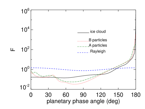
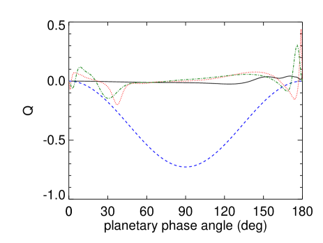
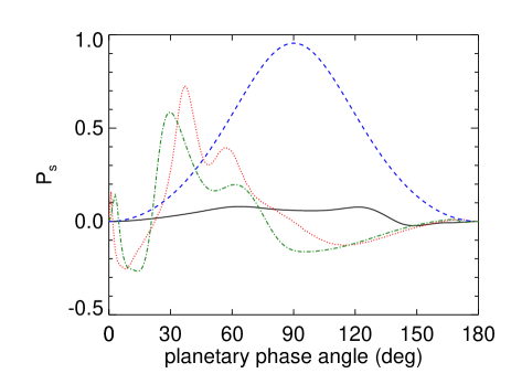
Figure 3: Single scattering phase function $F$, linearly polarized flux $Q$, and degree of linear polarization $P_{\mathrm{s}}$ as functions of the phase angle $\alpha$ ($\alpha=180^{\circ}-\Theta$, with $\Theta$ the single scattering angle). Linearly polarized flux $U$ equals zero, and $P_{\rm s}$ is defined as $-Q/F$. Curves are shown for liquid water droplets type A ($r_{\rm eff}=0.2\leavevmode\nobreak\ \mu$m, $v_{\rm eff}=0.1$), type B ($r_{\rm eff}=6.0\leavevmode\nobreak\ \mu$m, $v_{\rm eff}=0.4$), and water ice particles (Hess & Wiegner 1994; Hess 1998), all calculated at $\lambda=0.550\leavevmode\nobreak\ \mu$m. For comparison, the curves for Rayleigh scattered light are also shown.

Figure 3 shows the total flux, the polarized flux and the degree of linear polarization of light that has been singly scattered by the cloud droplets and the ice particles at a wavelength $\lambda$ equal to 0.550 $\mu$m, when the incident light is unpolarized. The curves for scattering by gas molecules (Rayleigh scattering) have also been added. All curves have been plotted as functions of the phase angle $\alpha$ instead of of the more common single scattering angle $\Theta$ to facilitate the comparison with the signals of the planets. Since for single scattering by the spherical cloud particles or by the ensemble of randomly oriented ice crystals, the scattered light is oriented parallel or perpendicular to the scattering plane (the plane containing the directions of propagation of the incident and the scattered light), we use the signed degree of linear polarization $P_{\rm s}$ in Fig. 3: when $P_{\rm s}$ is larger (smaller) than 0, the direction of polarization is perpendicular (parallel) to the scattering plane. The absolute value of $P_{\rm s}$ equals $P$.

The curves for Rayleigh scattering by gas clearly show the nearly isotropic scattering of the total flux, the symmetry of the polarization phase function and the high polarization values around $\alpha=90^{\circ}$. The curves for the total flux scattered by both types of liquid water droplets have a strong forward scattering peak at the largest values of $\alpha$ (the smallest single scattering angles), which is due to refraction and depends mostly on the size of the scattering particles, and not so much on their shape (Mishchenko et al. 2010). Another characteristic of the flux phase function of the droplets is the primary rainbow, that is due to light that has been reflected once inside the particles. For a given wavelength, the precise location of the rainbow depends on the particle size: for the small type A particles, it is found close to $\alpha=30^{\circ}$, while for the larger type B particles, it is close to $\alpha=40^{\circ}$. The primary rainbow also shows up in the scattered polarized flux and very strongly in the degree of polarization $P_{\mathrm{s}}$. The direction of polarization across the primary rainbow is perpendicular to the planetary scattering plane. The polarized flux and $P_{\mathrm{s}}$ go through zero, thus change direction, a few times between phase angles of 0^∘ and 180^∘. These particular phase angles are usually referred to as neutral points and, like the rainbow, they depend on the particle properties and the wavelength. At 0.550 $\mu$m, the type A particles have neutral points at 5^∘, 20^∘, 76^∘ and 158^∘, and the type B particles at 2^∘, 22^∘, 94^∘, and 160^∘.

The total flux scattered by the ice particles (Hess & Wiegner 1994; Hess 1998) has a smooth appearance without a feature such as the rainbow but with a strong forward scattering peak at the largest values of $\alpha$. The polarized flux and the degree of polarization of the ice particles are also smooth functions of $\alpha$. The neutral point of the ice particles is around $\alpha=140^{\circ}$.

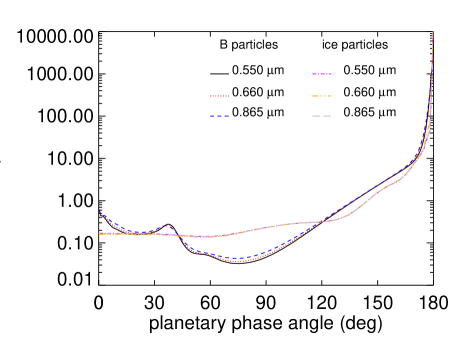
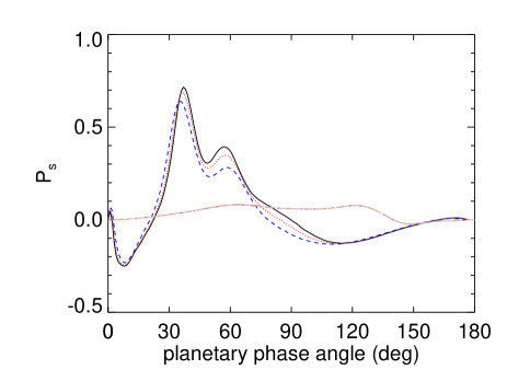
Figure 4: Singly scattered $F$, $Q$, and $P_{\mathrm{s}}$ as functions of $\alpha$ for the liquid water droplets type B and the ice particles at $\lambda=0.550$, $0.660$ and 0.865 $\mu$m. The curves for the ice particles overlap each other.

Fig. 4 shows the degree of linear polarization $P_{\mathrm{s}}$ for the type B liquid water droplets and the ice particles at $\lambda=0.550$, $0.660$ and 0.865 $\mu$m. The ice particles are relatively large, and therefore their scattering properties are virtually insensitive to $\lambda$ across the wavelength region of our interest (the visible). The scattering properties of the liquid cloud particles vary slightly with the wavelength: with increasing $\lambda$, the strengths of the primary and secondary rainbows decreases slightly, and the neutral point around intermediate phase angles shifts towards smaller phase angles. With increasing $\lambda$, the primary rainbow also shifts towards smaller phase angles (larger single scattering angles). As also discussed in Karalidi et al. (2011), the dispersion of the primary rainbow depends on the size of the particles that scatter the incident starlight: in large particles, such as rain droplets, the dispersion shows the opposite behavior, with the primary rainbow shifting towards larger phase angles with increasing $\lambda$. This latter shift gives rise to the well–known primary rainbow seen in the rainy sky with the red bow on top and the violet bow at the bottom.

3 The influence of the liquid water cloud coverage

In this section, we explore the strength of the primary rainbow feature as a function of the liquid water cloud coverage. All clouds have the same optical thickness, i.e. 2.0 (at 0.550 $\mu$m), and the same altitudes of their bottoms and tops, i.e. 3 and 4 km, respectively (see Fig. 1). The clouds consist of type A droplets.

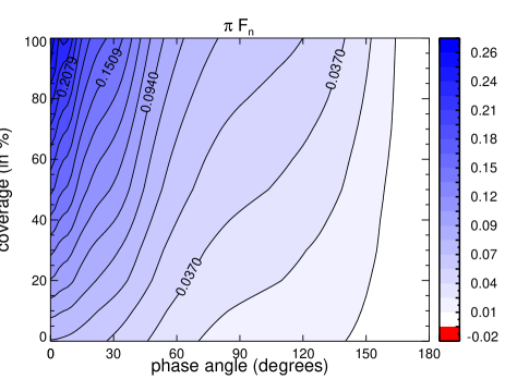
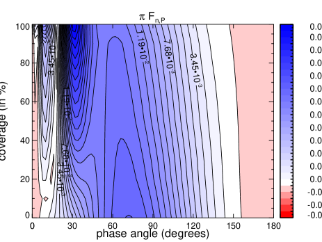
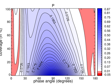
Figure 5: The total flux $\pi F_{\mathrm{n}}$, the polarized flux $\pi F_{\mathrm{n,P}}$, and the degree of polarization $P$ as functions of the phase angle $\alpha$ for liquid water cloud coverages from 0% up to 100%. Wavelength $\lambda$ is 0.550 $\mu$m, the optical thickness of the clouds is 2.0, and their top is at 4 km. The clouds are composed of type A droplets.

Figure 5 shows the total reflected flux $\pi F_{\mathrm{n}}$, the polarized reflected flux $\pi F_{\mathrm{n,P}}$, and the degree of polarization $P$ at 0.550 $\mu$m, as functions of the phase angle $\alpha$ and the percentage of cloud coverage. Horizontal cuts through Fig. 5 at a number of coverages are shown in Fig. 6. Because the model planets are not mirror–symmetric with respect to the planetary scattering plane, we use Eq. 3 to define the degree of polarization instead of the $P_{\mathrm{s}}$ used in the previous section.

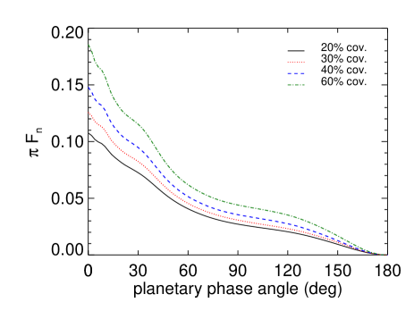
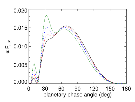
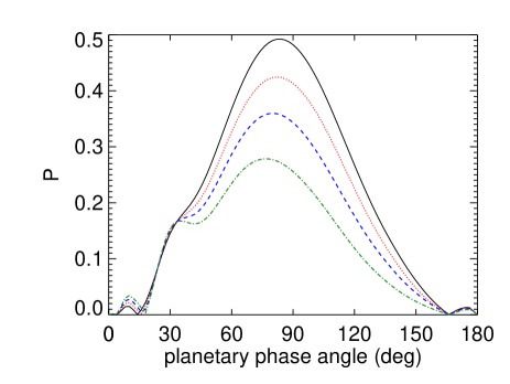
Figure 6: Horizontal cuts through the panels of Fig. 5 for cloud coverages of 20%, 30%, 40%, and 60%.

Clearly, as the cloud coverage increases, the flux and polarization features converge smoothly towards the signals for completely cloudy planets (see also Karalidi et al. 2011, for flux and polarization signals of completely cloudy planets). At small coverages, $P$ has a strong maximum around $\alpha=90^{\circ}$, which is due to scattering by the gas molecules above and between the patchy clouds. The Rayleigh scattering optical thickness above the clouds is 0.06 at $\lambda=0.550\leavevmode\nobreak\ \mu$m, and between the clouds, it is 0.097 (see Sect. 2.3). As expected from the single scattering curves (Fig. 3), the primary rainbow feature is located close to $\alpha=30^{\circ}$. The precise rainbow phase angle depends on the size of the particles and the wavelength, but, as expected, it does not depend on the cloud coverage.

In the total flux $\pi F_{\mathrm{n}}$, the rainbow is difficult to discern regardless of the cloud coverage (Fig. 5), as can also be seen in Fig. 6. In the polarized flux, the rainbow shows up as a local maximum for coverages of about 30% or more. In the degree of polarization, $P$, the rainbow feature is a shoulder on the Rayleigh scattering maximum from a cloud coverage of $\sim$20%. For a cloud coverage larger than about 40%, the rainbow causes a local maximum in $P$, because the Rayleigh scattering maximum decreases with increasing cloud coverage. A reflecting (i.e. non–black) surface underneath our atmosphere would increase the contrast of the (primary) rainbow peak by lowering the intensity of the Rayleigh scattering peak due to the increase of light with a generally low degree of polarization.

At phase angles near 20^∘, $\pi F_{\mathrm{n,P}}$ and $P$ are close to zero, fairly independent of the cloud coverage (see Fig. 6). This phase angle corresponds to a neutral point in the single scattering polarization phase function (Fig. 3). The type A cloud particle’s neutral point near 76^∘ is lost in the Rayleigh scattering contribution to $P$. The neutral point near 5^∘ yields the near–zero polarization region at the smallest phase angles, while the neutral point near 158^∘ and the generally low polarization values at those phase angles (see Fig. 3) show up as the broad low $P$ region at the largest phase angles in Fig. 5. Note that at these largest phase angles, the planet is almost in front of its star, and will be extremely difficult to detect directly anyway.

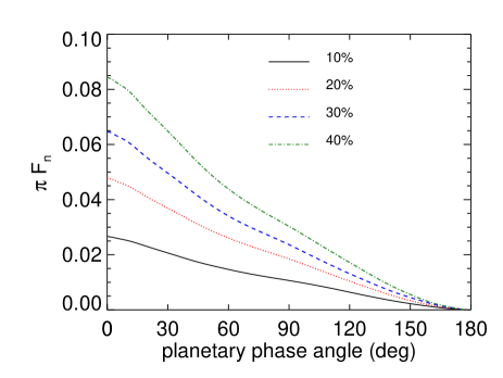
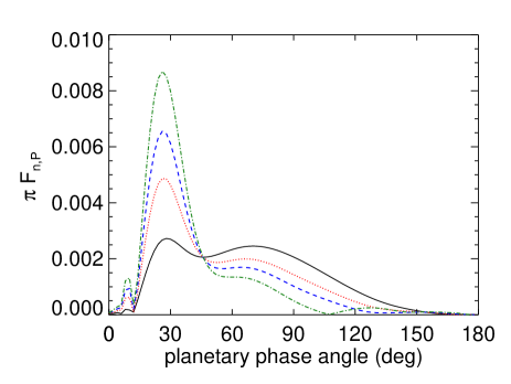
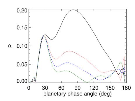
Figure 7: Similar to Fig. 6, except for $\lambda=0.865\leavevmode\nobreak\ \mu$m.

Figure 7 shows the same as Fig. 6, except for $\lambda=0.865\leavevmode\nobreak\ \mu$m. At this wavelength, the Rayleigh scattering optical thickness above the clouds is 0.01, while between the clouds it is 0.016 (see Sect. 2.3). The optical thickness of the clouds at 0.865 $\mu$m is 2.1. The differences in reflected fluxes and the degree of polarization between Fig. 7 and Fig. 6 are due to the difference in Rayleigh optical thickness above and between the clouds and to the difference in scattering properties of the cloud particles at the different wavelengths. Note that the effects of lowering the Rayleigh scattering optical thickness above the clouds are similar to increasing the altitude of the clouds.

At 0.865 $\mu$m, the reflected total flux $\pi F_{\mathrm{n}}$ is a very smooth function of $\alpha$, almost without even a hint of the rainbow. This smoothness is due to the smoother single scattering phase function of the small type A particles at this relatively long wavelength. The degree of polarization shows a very strong rainbow signature, especially for cloud coverages larger than 10%. The reason that the rainbow is so strong is mostly due to the small Rayleigh scattering optical thickness above the clouds, which suppresses the strong polarization maximum around 90^∘. The strength of the rainbow appears to be fairly independent of the percentage of coverage (all clouds have the same optical thickness). Around $\alpha=108^{\circ}$, $P$ is virtually zero for a coverage of 40%. These low values of $P$ (also in the graphs for the 20% and 30% coverage, but then around $\alpha=135^{\circ}$ and 130^∘, respectively) are due to the direction of polarization of the light scattered by the cloud particles (cf. Figs. 3 and 4) that is opposite to that of light scattered by the gas molecules. Because at 0.865 $\mu$m, the Rayleigh scattering optical thickness is small, the single scattering polarization signatures of the ice particles dominate the polarization signature of the planet.

4 The influence of mixed cloud droplet sizes

In the previous section, all clouds were composed of the same type of liquid water cloud droplets. In reality, cloud droplet sizes vary across the Earth. Typically, droplets above continents are smaller than those above oceans, due to different types of condensation nuclei and different amounts of condensation nuclei. In particular, typical cloud particle radii range from about $5\leavevmode\nobreak\ \mu$m to $30\leavevmode\nobreak\ \mu$m, with a global mean value of about $8.5\leavevmode\nobreak\ \mu$m above continental areas, and $11.8\leavevmode\nobreak\ \mu$m above maritime areas (Han et al. 1994). Also within clouds, droplet size distributions will vary, depending e.g. on internal convective updrafts or downdrafts that influence droplet growth through condensation and collisions (see e.g. Stephens & Platt 1987; Spinhirne et al. 1989). Here, we will present the influence of clouds with different liquid water droplet size distributions on the flux and polarization signals of a model planet.

Our model planet has two layers of clouds, with the lower clouds located between 1 and 3 km (0.902 and 0.710 bar) and the upper clouds between 3 and 4 km (0.710 and 0.628 bar) (cf. Fig. 1). The lower clouds are composed of the type B droplets ($r_{\mathrm{eff}}=6.0\mu$m, $v_{\mathrm{eff}}=0.4$) and have a coverage of 42.3%. The upper clouds are composed of the smaller, type A droplets ($r_{\mathrm{eff}}=2.0\mu$m, $v_{\mathrm{eff}}=0.1$) and have a coverage of 16%. The maps for the upper and the lower clouds were generated separately and hence there are regions with only lower clouds, or only upper clouds, or both.

Figure 8: $\pi F_{\mathrm{n}}$, $\pi F_{\mathrm{n,P}}$, and $P$ as functions of $\alpha$ for a planet with a lower, type B liquid water cloud that covers $\sim$42.3% and an upper, type A liquid water cloud layer that covers $\sim$16% of the planet for various values of the cloud optical thicknesses.

Figure 8 shows the reflected total flux $\pi F_{\mathrm{n}}$, the polarized flux $\pi F_{\mathrm{n,P}}$, and the degree of polarization $P$ for our model planet at $\lambda=0.550\leavevmode\nobreak\ \mu$m for different values of the cloud optical thickness, $b$. Because the two types of cloud particles have slightly different locations of the rainbows, the rainbow in the total flux in the presence of two cloud layers appears to be somewhat broadened, as compared to the curves for the fluxes of single layers of clouds (the curves in Fig. 8 where one of the cloud optical thicknesses equals zero).

In $P$, the strength of the rainbow feature appears to depend on the properties of the highest cloud layer: adding a lower cloud layer mainly decreases the strength of the Rayleigh scattering maximum by adding more low polarized light at these phase angles. $P$ is fairly insensitive to the optical thickness of this lower cloud layer (i.e. 2 or 10): increasing the thickness of this cloud slightly increases $\pi F_{\mathrm{n}}$, but also slightly increases $\pi F_{\mathrm{n,P}}$. This latter effect can also be seen in the rainbow feature in the curves for a planet with a single, lower cloud layer: with increasing $b$, $\pi F_{\mathrm{n}}$ increases, but $\pi F_{\mathrm{n,P}}$ increases, too! At larger phase angles ($\alpha>55^{\circ}$ in Fig. 8), increasing $b$ of the lower cloud layer increases $\pi F_{\mathrm{n}}$ but does not increase $\pi F_{\mathrm{n,P}}$ significantly, which can be attributed to the single scattering properties of the cloud droplets (see Fig. 3).

5 The influence of the ice cloud coverage

On Earth, liquid water clouds can be overlaid by water ice clouds. These latter clouds can be entirely separate (such as high-altitude cirrus clouds) or the upper parts of vertically extended clouds that have lower parts consisting of liquid water droplets. The amount of ice cloud coverage on Earth depends strongly on the latitude. Cirrus clouds for example, have an annual mean coverage of $\sim$20% in the tropics, while at northern mid-latitudes the annual mean coverage goes down to $\sim$12%. Globally, cirrus clouds cover $\sim$14% of the Earth’s upper troposphere (Eleftheratos et al. 2007). As mentioned in Sect. 1, water ice particles come in various sizes and shapes that yield single scattering properties that differ from those of liquid water droplets. In particular, light that has been singly scattered by ice cloud particles does not show a rainbow feature between phase angles of 30^∘ and 40^∘ (i.e. between single scattering angles of 140^∘ and 150^∘).

To investigate the influence of water ice clouds on the strength of the rainbow feature of liquid water clouds, we used model planets with two layers of clouds: a lower layer of optical thickness 10, consisting of type B liquid water droplets and an upper layer containing water ice particles Hess & Wiegner (1994); Hess (1998). The lower layer is located between 279 and 273 K (3 and 4 km, or 0.710 and 0.628 bar) and the upper layer between 253 and 248 K (7 and 8 km, or 0.426 and 0.372 bar) (c.f. Fig. 1). The single scattering properties of the water ice particles clouds have been calculated using the code of Hess & Wiegner (1994); Hess (1998). The singly scattered total and polarized flux and the degree of polarization of our ice cloud particles are shown in Fig. 3 for $\lambda=0.550\leavevmode\nobreak\ \mu$m and in Fig. 4 for $\lambda=0.660$ and 0.865$\leavevmode\nobreak\ \mu$m.

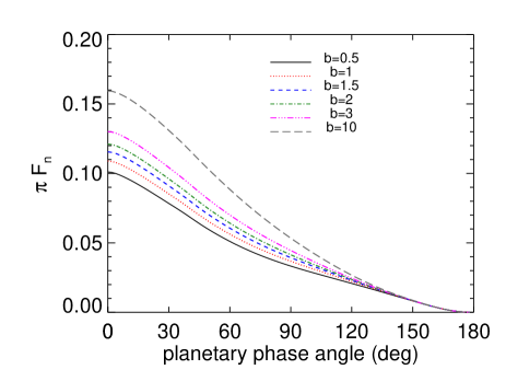
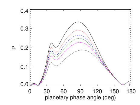
Figure 9: $\pi F_{\mathrm{n}}$ and $P$ as functions of $\alpha$ at $\lambda=0.550\leavevmode\nobreak\ \mu$m, for a planet with a lower liquid water cloud with $b=10$ that covers $\sim$42.3% of the planet and an upper ice cloud layer that covers $\sim$16% of the planet, and $\sim$11% of the liquid water clouds.

Our first model planets have a liquid water cloud layer that covers $\sim$ 42.3% of the surface, and an ice cloud layer that covers $\sim$ 16%. About 4.5% of the liquid water clouds is covered by ice clouds (i.e. $\sim$ 12% of the ice clouds is covering a liquid water cloud). Figure 9 shows $\pi F_{\mathrm{n}}$ and $P$ of our model planets as functions of $\alpha$ for various optical thicknesses of the ice clouds.

Adding a thin ice cloud (with $b=0.5$) to the cloudy planet lowers $\pi F$ at the smallest phase angles (cf. Fig. 8), because the ice particles are less less strong backward scattering than the liquid water droplets (cf. Fig. 3). At intermediate phase angles (around $\alpha=90^{\circ}$), the thin ice clouds brighten the planet, because at those angles, their single scattering phase function is higher than that of the liquid water droplets (cf. Fig. 3). Clearly, with increasing ice cloud optical thickness the reflected flux increases across the whole phase angle range (which is difficult to see at phase angles larger than about 150^∘).

The total flux $\pi F_{\mathrm{n}}$ does not show any evidence of a rainbow feature, not even for the thinnest ice cloud. The degree of polarization $P$, however, clearly shows the signature of the rainbow, even for large optical thicknesses of the ice cloud particles (cf. Fig. 9). The rainbow shows up in $P$ despite the overlaying ice clouds, because the ice particles themselves have a very low polarization signature especially in the phase angle region of the rainbow (see Fig. 3), so the only polarized signals arise from scattering by the liquid cloud particles and the gas molecules (which yields the maximum in $P$ around 90^∘). Increasing the ice cloud optical thickness, decreases $P$ across all phase angles because it increases the amount of mostly unpolarized reflected light.

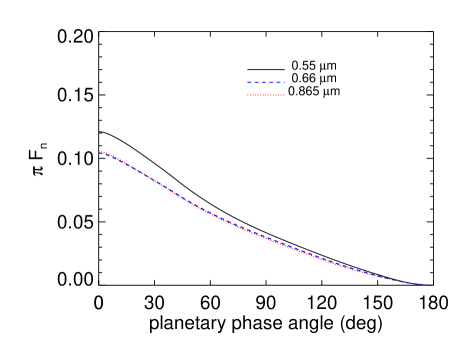
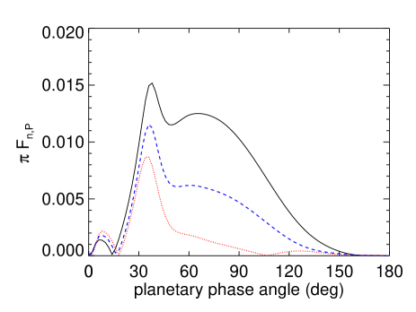
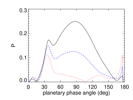
Figure 10: Similar to Fig. 9, except for an ice cloud with $b=2.0$, and for $\lambda=0.550$, 0.660, and 0.865 $\mu$m. The $\pi F_{\rm n}$ curves for 0.660 and 0.865 $\mu$m overlap.

In Fig. 10, we have plotted $\pi F_{\mathrm{n}}$, $\pi F_{\mathrm{n,P}}$ and $P$ for the same model planet as used for Fig. 9, except for an ice cloud optical thickness of 2.0, and for $\lambda=0.660$ and 0.865 $\mu$m. For comparison, the $\lambda=0.550$ $\mu$m curves (see Fig. 9) are also shown. With increasing wavelength, the total reflected flux decreases, mainly because the Rayleigh scattering optical thickness above and between the clouds decreases. The decrease of the Rayleigh scattering optical thickness is also apparent from the decrease of the maximum in $P$ around 90^∘, and the stronger influence of the single scattering polarization phase function of the liquid water cloud droplets. The ice particles leave no obvious feature in the polarization phase function at longer wavelengths, except that they decrease $P$ somewhat as compared to $P$ of a planet with only a liquid cloud (cf. the 40% coverage curve in Fig. 7).

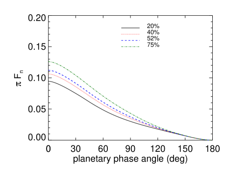
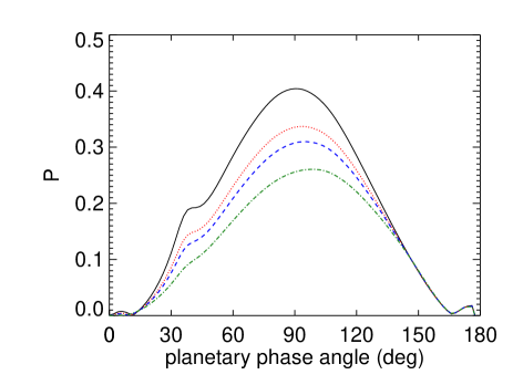
Figure 11: Similar to Fig. 9, except for a lower liquid water cloud that covers $\sim$25% of the planet and an upper ice cloud with $b=4.0$. The ice cloud coverage is varied from 20% to 75% of the water clouds.

To investigate the influence of the ice cloud coverage over liquid water clouds on the reflected flux and polarization, we used a model planet with lower liquid water clouds with $b=10$ and a coverage of $\sim\leavevmode\nobreak\ 25$%, and upper ice clouds with $b=4$ right above the liquid water clouds. Figure 11 shows the planet’s flux and polarization phase functions at $\lambda=0.550\leavevmode\nobreak\ \mu$m for various ice cloud coverages of the liquid water clouds (thus, an ice cloud coverage of 75% of the liquid water clouds, equals an ice cloud coverage of $\sim$16% of the planet).

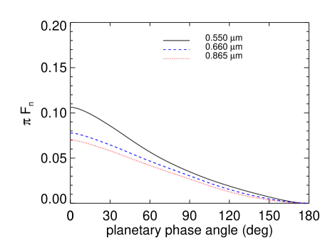
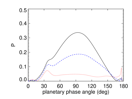
Figure 12: Similar to Fig. 11, for ice clouds covering 40% of the liquid water clouds, and for $\lambda=0.550$, 0.660, and 0.865 $\mu$m.

Even with ice clouds covering as little as 20% of the liquid water clouds (5% of the planet, but only above the liquid water clouds), the total flux phase function fails to show a hint of the rainbow. This was also apparent from Fig. 9, where 11% of the liquid water clouds was covered by an ice cloud. The polarization phase function does show the rainbow feature, but up from an ice cloud coverage of 40% (a coverage of 10% of the planet) in Fig. 9, the feature is increasingly weak such that it disappears into the Rayleigh scattering polarization maximum around 90^∘. At longer wavelengths, such as 0.865 $\mu$m, where the Rayleigh scattering optical thickness above and between the clouds is smaller, the rainbow feature is still clearly visible in $P$ when ice clouds cover 40% of the liquid water clouds. This can be seen in Fig. 12.

6 Looking for the rainbow on Earth

Figure 11 shows us that liquid water clouds on a planet can be detected using polarization measurements of the reflected starlight, even when the liquid water clouds are (partly) covered by water ice clouds. The question arises whether the rainbow would be visible for a distant observer of the Earth. As far as we know, the only polarization observations of the Earth have been done by the POLDER instrument (POLarization and Directionality of the Earth’s Reflectances) a version of which is currently flying onboard the PARASOL satellite (for a description of the instrument, see Deschamps et al. 1994). Locally, POLDER has indeed observed the primary rainbow above liquid water clouds (see Goloub et al. 2000). However, since PARASOL is in a low–Earth–orbit, the POLDER measurements are not representative for polarization observations of the whole (disk–integrated) Earth observed from afar.

Table 1: The cloud optical thicknesses $b$ (at $\lambda=0.550\leavevmode\nobreak\ \mu$m) from the MODIS/Aqua data from April 25, 2011. To avoid having to include too many different values of $b$, we have binned the optical thicknesses as shown below. Ice clouds with $b\geq 20$ are ignored.

Liquid water cloud		Ice water cloud
$b_{\mathrm{MODIS}}$	$b_{\mathrm{model}}$	$b_{\mathrm{MODIS}}$	$b_{\mathrm{model}}$
$0<b<1$	0.5	$0<b<1$	0.5
$1\leq b<10$	5	$1\leq b<2$	1.5
$5\leq b<20$	15	$2\leq b<5$	3
$20\leq b<50$	35	$5\leq b<10$	7.5
$50\leq b<80$	65	$10\leq b<20$	15

In the absence of real polarization observations, we have simulated the total flux and polarization of light reflected by the whole Earth using cloud properties derived from observations by MODIS (Moderate Resolution Imaging Spectroradiometer), onboard NASA’s Aqua satellite. We used MODIS’ cloud coverage (the horizontal distribution of the clouds), cloud thermodynamic phase (liquid or ice), and the cloud optical thickness as measured on April 25th, 2011, to build a model Earth. To limit the number of (time–consuming) calculations, we binned the measured optical thicknesses according to Table 1. Ice clouds with an optical thicknesses larger than 20 (at $\lambda=0.550\leavevmode\nobreak\ \mu$m) were ignored, so as to include only cirrus/cirrostratus ice clouds in our sample (according to the ISCCP categorization) and to avoid deep convection clouds. We assume that the liquid water clouds consist of the type B droplets and for the ice particles, we use the models of Hess & Wiegner (1994) and Hess (1998). Finally, our ice clouds are positioned at altitudes with temperatures lower than 253 K, so that we avoid mixed–phase clouds (in which droplets and crystals exist side–by–side). The surface is assumed to be black as an ocean.

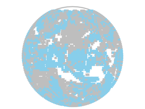
Figure 13: The cloud map of the Earth on April 25th, 2011, based on MODIS/Aqua data. The planet is covered by $\sim$63% liquid water clouds (gray regions) and $\sim$36% ice clouds (blue regions). About 28% of the planet is covered by two layers of clouds.

Figure 13 shows the cloud map of our model Earth. On April 25th, 2011, about 85% of the planet was covered by clouds (liquid and/or ice), about 14% was covered by both liquid and ice clouds, about 63% of the planet was covered by liquid water clouds and about 36% by water ice clouds.

In Fig. 14, we show the calculated $\pi F_{\mathrm{n}}$ and $P$ of our model Earth at $\lambda=0.550\leavevmode\nobreak\ \mu$m and 0.865 $\mu$m. The total reflected flux at $\alpha=0^{\circ}$ equals the planet’s geometric albedo, which is very similar at the two wavelengths and equals $\sim$0.22 at $\lambda=0.55\leavevmode\nobreak\ \mu$m. This value is slightly smaller than the one found in literature for Earth’s geometric albedo (0.33 (Brown 2005)) and is due to our use of a black surface on our planet. It is clear that the total reflected flux does not show a rainbow feature, while the degree of polarization does. The maximum $P$ in the rainbow feature is 0.08 (8% in polarization) at $\lambda$=0.55 $\mu$m, and the absolute difference with the nearby local minimum around $\alpha=50^{\circ}$, is 0.02 in $P$ (an absolute difference of 2% in polarization). At $\lambda=0.865\leavevmode\nobreak\ \mu$m, the rainbow feature is even more pronounced in $P$, with an absolute difference with its surroundings of more than 4 $\%$. Interestingly, $P$ reaches zero around the rainbow feature (which indicates a change of direction of the polarization), which should facilitate measuring the strength of the rainbow feature.

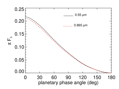
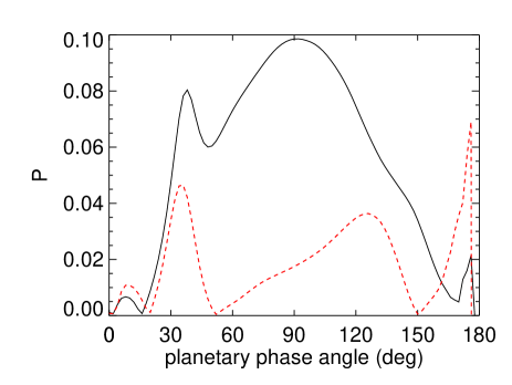
Figure 14: $\pi F_{\mathrm{n}}$ and $P$ as functions of $\alpha$ for the model Earth with clouds as shown in Fig. 13.

Bailey (2007) derived the disk-integrated polarization signature of the partly-cloudy Earth from remote-sensing data and predicted degrees of polarization of $\sim$12.7% to $\sim$15.5% in the rainbow peak at wavelengths between about 0.5 to 0.8 microns. These values are higher than our values of 4% to 8% as shown in Fig. 14. The differences are, however, small when considering the estimations by Bailey (2007) on the influence of multiple scattering and ice clouds on the polarization.

7 Summary and conclusions

The flux and degree of linear polarization of sunlight that is scattered by cloud particles and that is reflected back to space depend on the phase angle. Close to a phase angle of 40^∘, the flux and degree of polarization of unpolarized incident light that is singly scattered by spherical water cloud droplets, shows the enhancement that is known as the primary rainbow. The multiple scattering of light within clouds dilutes the primary rainbow feature both in flux and in polarization. In Earth–observation, with a spatial resolution of a few kilometers, the detection of the polarized rainbow feature is used to discriminate between liquid water clouds and ice clouds (Goloub et al. 2000). Light that is scattered by ice cloud particles, such as hexagonal crystals, does not show the rainbow feature. Knowledge of the cloud properties (thermodynamical phase, optical thickness, microphysical properties etc) are crucial for studies of global climate change on Earth (Goloub et al. 2000).

In Karalidi et al. (2011), we used horizontally homogeneous model planets to investigate the strength of the rainbow feature in flux and polarization for various model atmospheres of terrestrial exoplanets. In that paper, we briefly discussed the influence of a second atmospheric layer containing clouds on top of another one and the implications that that could have on our ability to characterize the planetary atmosphere. We concluded that even when the upper cloud has a relatively small optical thickness, the polarization signal of the planet is mainly determined by the properties of the upper cloud particles. Here, in Sects. 4 and 5 we extended this research on horizontally inhomogeneous exoplanets and for various cloud cases.

We noticed that in case the cloud layers contain clouds of similar nature (for example liquid water clouds) and when the cloud particles present a size stratification with altitude it is the top cloud layer that will define the total planetary signal, as was also the case in Karalidi et al. (2011). On the other hand if the clouds are made out of the same nature and size particles it is the (optically) thickest clouds that will define to a largest extent the planetary signal.

In case the upper cloud layer contains ice clouds, we noticed that the characteristics of the planetary signal can depend on either one of the cloud layers, depending on their overcast and the optical thickness of the ice cloud layer. Using our homogeneous planet code we have seen that for $b_{\mathrm{ice}}\gtrsim 3$ the existence of any lower cloud on the observed planetary pixel will be masked. When the overcast of the two cloud layers is small the existence of the ice cloud layer does not seem to be able to cover the existence of the water cloud layer (i.e. the rainbow), even for high values of the optical thickness (see Fig. 9).

Even in case the ice cloud layer has an optical thickness large enough to mask the existence of the underlying liquid water cloud, the rainbow feature of the liquid water cloud survives for the case the ice cloud layer covers slightly more than half the water clouds (see Fig. 11). So unless our observed exoplanet contains a very large number of ice clouds in its atmosphere, the rainbow of the water clouds will still be visible in the planetary $P$ signal.

An interesting test–case for the detection of the rainbow is our own Earth. To test whether a distant observer would be able to detect a rainbow due to Earth’s liquid water clouds partly covered by water ice clouds, we modeled the Earth’s cloud coverage using MODIS/Aqua data from April 25, 2011. These data contained the location and optical thickness of ice and water clouds across the planet. We binned the cloud optical thicknesses in a limited number (5) of optical thickness values (to avoid too many time–consuming computations), as tabulated in Table 1, and modelled the scattering properties of the liquid water cloud droplets using Mie-scattering and those of the water ice crystals using the models of Hess (1998).

Our calculations for the disk–integrated flux and polarization signals of this model Earth as functions of the planetary phase angle and at $\lambda=0.550\leavevmode\nobreak\ \mu$m and 0.865 $\mu$m, show that the flux does not have the primary rainbow feature. Flux observations as a function of the phase angle would thus not provide an indication of the liquid water clouds on Earth. In the polarization signal, however, the rainbow is clearly visible, especially at the longer wavelengths ($\lambda=0.865\leavevmode\nobreak\ \mu$m). Polarimetry as a function of the planetary phase angle would thus establish the existence of liquid water clouds on our planet.

The results presented in this paper were for a black planetary surface. A bright surface that reflects light with a low degree of polarization would not significantly affect the reflected polarized flux, but it would increase the total flux, and hence decrease the degree of polarization. If a planet were thus covered by a bright surface and few clouds, the rainbow feature would be less strong than presented here (with increasing cloud coverage, the influence of the surface would decrease), although P at other phase angles would also be subdued. For example, comparing our results for a planet with a mean Earth cloud coverage completely covered by a sandy surface with an albedo of 0.243 (at 0.55 $\mu$m), polarization in the rainbow would be about 15.39%, compared to 41.7% for a planet completely covered by a black surface. Detailed calculations for planets with realistically inhomogeneous surfaces and inhomogeneous cloud decks, preferably including the variations of the cloud deck in time, would help to study the effects of the surface reflection. With an ocean surface with waves, one could also expect the glint of starlight to contribute to the reflected flux and polarization (Williams & Gaidos 2008). How often this glint would be visible through broken clouds and its effect on the rainbow of starlight that is scattered by cloud particles, when it is indeed visible, will be subject to further studies.

Summarizing, the primary rainbow of starlight that has been scattered by liquid water clouds should be observable for modest coverages (10% - 20%) of liquid clouds, and even when liquid water clouds are partly covered by water ice clouds. The total flux of the reflected starlight as a function of the planetary phase angle does not show the rainbow feature due to the presence of ice clouds. The degree of linear polarization of this light as a function of the phase angle will usually show the rainbow feature, even when a large fraction (up to $\sim$50%) of the liquid water clouds are covered by ice clouds. Polarimetry of starlight that is reflected by exoplanets, thus provides a strong tool for the detection of liquid water clouds in the planetary atmospheres.

References

- Baglin et al. (2006) Baglin, A., Auvergne, M., Barge, P., et al. 2006, in ESA Special Publication, Vol. 1306, ESA Special Publication, ed. M. Fridlund, A. Baglin, J. Lochard, & L. Conroy, 33
- Bailey (2007) Bailey, J. 2007, Astrobiology, 7, 320
- Berdyugina et al. (2008) Berdyugina, S. V., Berdyugin, A. V., Fluri, D. M., & Piirola, V. 2008, ApJ, 673, L83
- Berdyugina et al. (2011) Berdyugina, S. V., Berdyugin, A. V., Fluri, D. M., & Piirola, V. 2011, ApJ, 728, L6
- Brogi et al. (2012) Brogi, M., Snellen, I. A. G., de Kok, R. J., et al. 2012, Nature, 486, 502
- Brown (2005) Brown, R. A. 2005, ApJ, 624, 1010
- Cowan et al. (2009) Cowan, N. B., Agol, E., Meadows, V. S., et al. 2009, ApJ, 700, 915
- de Haan et al. (1987) de Haan, J. F., Bosma, P. B., & Hovenier, J. W. 1987, A&A, 183, 371
- de Mooij et al. (2012) de Mooij, E. J. W., Brogi, M., de Kok, R. J., et al. 2012, A&A, 538, A46
- de Rooij & van der Stap (1984) de Rooij, W. A. & van der Stap, C. C. A. H. 1984, A&A, 131, 237
- Deming et al. (2011) Deming, D., Knutson, H., Agol, E., et al. 2011, ApJ, 726, 95
- Deming et al. (2012) Deming, D., Fraine, J. D., Sada, P. V., et al. 2012, ApJ, 754, 106
- Deschamps et al. (1994) Deschamps, P.-Y., Breon, F.-M., Leroy, M., et al. 1994, IEEE Transactions on Geoscience and Remote Sensing, 32, 598
- Dohlen et al. (2008) Dohlen, K., Langlois, M., Saisse, M., et al. 2008, in Society of Photo-Optical Instrumentation Engineers (SPIE) Conference Series, Vol. 7014, Society of Photo-Optical Instrumentation Engineers (SPIE) Conference Series
- Ehrenreich et al. (2007) Ehrenreich, D., Hébrard, G., Lecavelier des Etangs, A., et al. 2007, ApJ, 668, L179
- Eleftheratos et al. (2007) Eleftheratos, K., Zerefos, C. S., Zanis, P., et al. 2007, Atmospheric Chemistry & Physics Discussions, 7, 93
- Ford et al. (2001) Ford, E. B., Seager, S., & Turner, E. L. 2001, Nature, 412, 885
- Goloub et al. (2000) Goloub, P., Herman, M., Chepfer, H., et al. 2000, J. Geophys. Res., 105, 14747
- Goode et al. (2001) Goode, P. R., Qiu, J., Yurchyshyn, V., et al. 2001, Geochim. Res. Lett., 28, 1671
- Han et al. (1994) Han, Q., Rossow, W. B., & Lacis, A. A. 1994, Journal of Climate, 7, 465
- Hansen & Hovenier (1974) Hansen, J. E. & Hovenier, J. W. 1974, Journal of Atmospheric Sciences, 31, 1137
- Hansen & Travis (1974) Hansen, J. E. & Travis, L. D. 1974, Space Science Reviews, 16, 527
- Hess (1998) Hess, M. 1998, J. Quant. Spec. Radiat. Transf., 60, 301
- Hess & Wiegner (1994) Hess, M. & Wiegner, M. 1994, Appl. Opt., 33, 7740
- Heymsfield & Platt (1984) Heymsfield, A. J. & Platt, C. M. R. 1984, Journal of Atmospheric Sciences, 41, 846
- Hovenier et al. (2004) Hovenier, J. W., Van der Mee, C., & Domke, H. 2004, Astrophysics and Space Science Library, Vol. 318, Transfer of polarized light in planetary atmospheres : basic concepts and practical methods, Kluwer Academic Publishers (Springer), Dordrecht
- Kaltenegger & Traub (2009) Kaltenegger, L. & Traub, W. A. 2009, ApJ, 698, 519
- Karalidi & Stam (accepted) Karalidi, T. & Stam, D. M. accepted for publication A&A
- Karalidi et al. (2011) Karalidi, T., Stam, D. M., & Hovenier, J. W. 2011, A&A, 530, A69+
- Kemp et al. (1987) Kemp, J. C., Henson, G. D., Steiner, C. T., & Powell, E. R. 1987, Nature, 326, 270
- Koch et al. (1998) Koch, D. G., Borucki, W., Webster, L., et al. 1998, in Presented at the Society of Photo-Optical Instrumentation Engineers (SPIE) Conference, Vol. 3356, Society of Photo-Optical Instrumentation Engineers (SPIE) Conference Series, ed. P. Y. Bely & J. B. Breckinridge, 599–607
- Macintosh et al. (2008) Macintosh, B. A., Graham, J. R., Palmer, D. W., et al. 2008, in Society of Photo-Optical Instrumentation Engineers (SPIE) Conference Series, Vol. 7015, Society of Photo-Optical Instrumentation Engineers (SPIE) Conference Series
- Macke et al. (1996) Macke, A., Mueller, J., & Raschke, E. 1996, Journal of Atmospheric Sciences, 53, 2813
- Magono & Lee (1966) Magono, C. & Lee, C. W. 1966, Journal of the Faculty of Science, Hokkaido University
- Marley et al. (2010) Marley, M. S., Saumon, D., & Goldblatt, C. 2010, ApJ, 723, L117
- Marshak et al. (2008) Marshak, A., Wen, G., Coakley, J. A., et al. 2008, Journal of Geophysical Research (Atmospheres), 113, 14
- Mayor & Queloz (1995) Mayor, M. & Queloz, D. 1995, Nature, 378, 355
- McClatchey et al. (1972) McClatchey, R. A., Fenn, R., Selby, J. E. A., Volz, F., & Garing, J. S. 1972, AFCRL-72.0497 (US Air Force Cambridge research Labs)
- Mishchenko (1990) Mishchenko, M. I. 1990, Icarus, 84, 296
- Mishchenko et al. (2010) Mishchenko, M. I., Rosenbush, V. K., Kiselev, N. N., et al. 2010, ArXiv e-prints
- Montañés-Rodríguez et al. (2006) Montañés-Rodríguez, P., Pallé, E., Goode, P. R., & Martín-Torres, F. J. 2006, ApJ, 651, 544
- Oakley & Cash (2009) Oakley, P. H. H. & Cash, W. 2009, ApJ, 700, 1428
- Pallé et al. (2008) Pallé, E., Ford, E. B., Seager, S., Montañés-Rodríguez, P., & Vazquez, M. 2008, ApJ, 676, 1319
- Pallé et al. (2004) Pallé, E., Goode, P. R., Montañés-Rodríguez, P., & Koonin, S. E. 2004, Science, 304, 1299
- Pepe et al. (2004) Pepe, F., Mayor, M., Queloz, D., et al. 2004, A&A, 423, 385
- Roelfsema et al. (2011) Roelfsema, R., Gisler, D., Pragt, J., et al. 2011, in Society of Photo-Optical Instrumentation Engineers (SPIE) Conference Series, Vol. 8151, Society of Photo-Optical Instrumentation Engineers (SPIE) Conference Series
- Saar & Seager (2003) Saar, S. H. & Seager, S. 2003, in Astronomical Society of the Pacific Conference Series, Vol. 294, Scientific Frontiers in Research on Extrasolar Planets, ed. D. Deming & S. Seager, 529–534
- Seager et al. (2000) Seager, S., Whitney, B. A., & Sasselov, D. D. 2000, ApJ, 540, 504
- Snellen et al. (2010) Snellen, I. A. G., de Kok, R. J., de Mooij, E. J. W., & Albrecht, S. 2010, Nature, 465, 1049
- Spinhirne et al. (1989) Spinhirne, J. D., Boers, R., & Hart, W. D. 1989, Journal of Applied Meteorology, 28, 81
- Stam (2003) Stam, D. M. 2003, in ESA Special Publication, Vol. 539, Earths: DARWIN/TPF and the Search for Extrasolar Terrestrial Planets, ed. M. Fridlund, T. Henning, & H. Lacoste, 615–619
- Stam (2008) Stam, D. M. 2008, A&A, 482, 989
- Stam et al. (2006) Stam, D. M., de Rooij, W. A., Cornet, G., & Hovenier, J. W. 2006, A&A, 452, 669
- Stam & Hovenier (2005) Stam, D. M. & Hovenier, J. W. 2005, A&A, 444, 275
- Stam et al. (2004) Stam, D. M., Hovenier, J. W., & Waters, L. B. F. M. 2004, A&A, 428, 663
- Stephens & Platt (1987) Stephens, G. L. & Platt, C. M. R. 1987, Journal of Applied Meteorology, 26, 1243
- Tinetti (2006) Tinetti, G. 2006, Origins of Life and Evolution of the Biosphere, 36, 541
- Tinetti et al. (2006) Tinetti, G., Meadows, V. S., Crisp, D., et al. 2006, Astrobiology, 6, 881
- Tinetti & Griffith (2010) Tinetti, G. & Griffith, C. A. 2010, in Astronomical Society of the Pacific Conference Series, Vol. 430, Astronomical Society of the Pacific Conference Series, ed. V. Coudé Du Foresto, D. M. Gelino, & I. Ribas, 115–+
- Tomasko et al. (2009) Tomasko, M. G., Doose, L. R., Dafoe, L. E., & See, C. 2009, Icarus, 204, 271
- van Diedenhoven et al. (2007) van Diedenhoven, B., Hasekamp, O. P., & Landgraf, J. 2007, Journal of Geophysical Research (Atmospheres), 112, 15208
- Wiktorowicz (2009) Wiktorowicz, S. J. 2009, ApJ, 696, 1116
- Williams & Gaidos (2008) Williams, D. M. & Gaidos, E. 2008, Icarus, 195, 927
- Zugger et al. (2010) Zugger, M. E., Kasting, J. F., Williams, D. M., Kane, T. J., & Philbrick, C. R. 2010, ApJ, 723, 1168
- Zugger et al. (2011) Zugger, M. E., Kasting, J. F., Williams, D. M., Kane, T. J., & Philbrick, C. R. 2011, ApJ, 739, 55