Bayesian Latent Variable Modeling of Longitudinal Family Data for Genetic Pleiotropy Studies

Abstract

Motivated by genetic association studies of pleiotropy, we propose here a Bayesian latent variable approach to jointly study multiple outcomes or phenotypes. The proposed method models both continuous and binary phenotypes, and it accounts for serial and familial correlations when longitudinal and pedigree data have been collected. We present a Bayesian estimation method for the model parameters, and we develop a novel MCMC algorithm that builds upon hierarchical centering and parameter expansion techniques to efficiently sample the posterior distribution. We discuss phenotype and model selection in the Bayesian setting, and we study the performance of two selection strategies based on Bayes factors and spike-and-slab priors. We evaluate the proposed method via extensive simulations and demonstrate its utility with an application to a genome-wide association study of various complication phenotypes related to type 1 diabetes.

Keywords: Bayesian inference, Genetics, Latent variable, Markov chain Monte Carlo, Path Sampling, Pleiotropy

1 Introduction

Pleiotropy occurs when a single genetic factor influences multiple continuous or binary phenotypes, and it is present in many genetic studies of complex human traits such as diabetes, hypertension and cardiovascular diseases. In genetic studies of complications or secondary manifestations of a disease, it is often believed that there are common genetic risk factors for the different phenotypes. In other cases, the primary and often conceptual phenotype (e.g. disease severity) may not be directly measured or be characterized by one single phenotype, and a set of surrogate response variables must instead be used. These response variables (phenotypes or outcomes) are mutually correlated as they measure the underlying trait from different perspectives. In order to take into account all information and to increase statistical efficiency, it is desirable to model these outcomes jointly.

An added characteristic of many emerging large-scale genetic studies is the collection of repeated measures over time in correlated individuals (family data). For example, the ongoing T2D-GENES (Type 2 Diabetes Genetic Exploration by Next-generation sequencing in multi-Ethnic Samples) consortium study includes longitudinal measures of various T2D-revelant phenotypes (e.g. blood glucose levels and blood pressures) and other covariates (e.g. sex, body mass index and medication history), and these measures are collected for 2,500 individuals from 85 Mexican-American families. Similarly, the DCCT (Diabetes Control and Complications Trial) study includes longitudinal measures of various type 1 diabetes (T1D) complications, which we analyze in this paper.

The longitudinal family studies combine the features of longitudinal studies in independent individuals and studies using single-time-point phenotype measures in families, providing more information about the genetic and environmental factors associated with the traits of interest than cross-sectional studies (Burton et al., 2005). However, joint modeling of multiple phenotypes using longitudinal family data involves non-trivial statistical and computational challenges because of the complex correlations that exist between different phenotypes (the phenotypical correlation), between repeated measures from the same phenotype (the serial correlation) and between individuals within the same family (the familial correlation).

Robust and powerful methods for the study of pleiotropy are under-developed in the literature due to data complexities that include a) the phenotypes of interest can be continuous, discrete or both, b) the joint effect of covariates on the multiple phenotypes is difficult to specify, and c) the familial, serial and other correlations are often present in the data as discussed above. There are a number of approaches proposed for cross-sectional data. For instance, Xu et al. (2003) extended the standard linear combination test to incorporate data-driven weighting factors, Weller et al. (1996) applied the principal component analysis to the multiple traits of interest to obtain independent canonical variables and then conducted univariate quantitative trait locus (QTL) analyses, and Lange and Whittaker (2001) developed a QTL-mapping method based on generalized estimating equations.

Here we propose to use the latent variable (LV) methodology to jointly study multiple correlated phenotypes in the presence of serial and familial correlations. The formulation of a latent variable model (LVM) relies on postulating the effect of a random variable that is not observed by the researchers but is assumed to exert an important influence on the set of observed variables (also known as the manifest variables) and thus induces correlations among them (Bartholomew et al., 2011). In the context of pleiotropy studies, the manifest variables are the multiple observed phenotypes, which jointly inform the latent variable that represents the underlying conceptual disease status or severity.

The LV methodology has been widely used in many scientific fields including economics, psychology and social sciences, and it is becoming increasingly attractive for genetic studies. For example, O’Hara et al. (2010) proposed a LV approach for the analysis of multivariate quantitative trait loci, Tayo et al. (2008) applied a factor analysis (a sub-type of LVM) to find latent common genetic components of obesity traits, and Nock et al. (2009) used the factor analysis for a metabolic syndrome study. Initial applications of LVM focused on reducing the number of manifest variables to a smaller number of latent outcomes. Sammel and Ryan (1996) and Sammel and Ryan (1997) extended the LVM to allow covariates to have effects on both the manifest and latent variables. Roy and Lin (2000) discussed a LV approach for longitudinal data with continuous outcomes.

The proposed LVM consists of two parts. The first part models the relationship between the manifest variables and the LV to characterize the within-subject correlation among the different outcomes. The second part uses a linear mixed effect model to investigate the effect of a genetic marker and other covariates on the LV, accounting for the serial and familial correlations. Direct effects of covariates on the manifest variables are also allowed in the first part of model.

The paper makes a number of original contributions. The proposed LV method generalizes the work of Roy and Lin (2000) to longitudinal family data with binary and continuous responses. The Bayesian formulation can be desirable in practice as it offers a principled way to incorporate prior information, often available in genetic studies, and to perform finite sample likelihood-based inference. However, the Bayesian model raises important computational challenges because the sampling algorithm required to study the posterior is inefficient when it is applied in its standard form. We introduce a novel algorithm that relies on the hierarchical centering and parameter expansion techniques (Gelfand, 1995; Liu and Wu, 1999; Meng and van Dyk, 1999) to improve computational efficiency.

The rest of the paper is organized as follows. Section 2 introduces the details of the LVM and discusses the consequences of naïvely ignoring the family structure in the data. Section 3 presents a Bayesian estimation for the model parameters and a novel MCMC algorithm designed to sample the posterior distribution efficiently. Section 4 discusses phenotype selection and model selection in the Bayesian setting. Section 5 shows results from extensive simulation studies, and Section 6 applies the proposed method to a genetic study of T1D complications. Section 7 concludes with recommendations and further discussions.

2 Latent Variable Model for Longitudinal Family data.

2.1 The Statistical Model

Let $\textbf{Y}_{cit}=(y_{cit1},\ldots,y_{citJ})^{{}^{\prime}}$ be the $J\times 1$ vector of outcomes/phenotypes/manifest variables measured at the $t^{th}$ time on the $i^{th}$ individual from the $c^{th}$ family/cluster for $c=1,2,\ldots,C$, $i=1,2,\ldots,N_{c}$, $t=1,2,\ldots,T$, where C denotes the total number of families, $N_{c}$ is the number of individuals within the $c^{th}$ family, and $T$ is the total number of repeated measurements. Among the $J$ outcomes, $\textbf{Y}^{c}_{cit}=(y^{c}_{cit1},\ldots,y^{c}_{citJ_{1}})^{{}^{\prime}}$ are continuous and $\textbf{Y}^{b}_{cit}=(y^{b}_{citJ_{1}+1},\ldots,y^{b}_{citJ})^{{}^{\prime}}$ are binary. Let $U_{cit}$ be the LV representing the conceptual disease severity which aggregates the partial information brought by each of the $J$ phenotypes.

In the first part of the LVM, a continuous phenotype $y^{c}$ is linked to the latent trait $U$ via a linear mixed model

$$y^{c}_{citj}=\beta_{0j}+W_{cit}^{T}\beta_{j}+\lambda_{j}U_{cit}+b_{cij}+e_{citj},$$ (2.1)

where $e_{citj}\stackrel{{\scriptstyle\text{iid}}}{{\sim}}N(0,\sigma^{2}_{j})$, $W_{cit}$ is a $p_{1}$-dimensional vector of covariates that have direct effects on the phenotype (direct fixed-effect covariates) and $\lambda_{j}$ is the factor loading that represents the effect of the LV on the $j^{th}$ phenotype. When all $\lambda_{j}$s are equal to 1, model (2.1) is reduced to a mixed effect model. The random component $b_{cij}$ captures the family-specific within-subject correlations over time. We assume $b_{cij}\stackrel{{\scriptstyle\text{iid}}}{{\sim}}N(0,\tau^{2}_{j})$, and $e_{citj}$ and $b_{cij}$ are mutually independent for $c=1,\ldots,C$, $i=1,\ldots,N_{c}$, $t=1,\ldots,T$ and $j=1,\ldots,J$.

If a phenotype is binary, a generalized linear mixed model is assumed,

$$\eta_{citj}=\beta_{0j}+W_{cit}^{T}\beta_{j}+\lambda_{j}U_{cit}+b_{cij},$$ (2.2)

with a probit link,

$$E\left[y^{b}_{citj}|U_{cit},b_{cij}\right]=p(y^{b}_{citj}=1|U_{cit},b_{cij})=\Phi(\eta_{citj}).$$ (2.3)

We choose a probit link instead of a logit link to gain computational efficiency. Specifically, we take advantage of the well-known representation of the probit model based on a normally distributed LV. If $\widetilde{y}^{b}_{citj}\sim N(\eta_{citj},1)$ is the Gaussian variable underlying the binary response $y^{b}_{citj}$, then (2.3) is recovered when $y^{b}_{citj}=\mathbf{1}_{\{\widetilde{y}^{b}_{citj}>0\}}$.

The second part of the LVM assess the effect of $X_{cit}$, a $p_{2}-$dimensional vector of variables that of primary interest (e.g. a genetic marker and possibly additional clinical factors), on the latent variable $U$ via a linear mixed model,

$$U_{cit}=X_{cit}^{T}\alpha+Z_{cit}^{T}a_{c}+Q_{cit}^{T}d_{ci}+\epsilon_{cit},$$ (2.4)

where $\epsilon_{cit}\stackrel{{\scriptstyle\text{iid}}}{{\sim}}N(0,\psi^{2})$. Elements in $X$ are also called indirect fixed-effect covariates because their effects on a phenotype of interest $Y$ is induced via the effect of the latent variable $U$ on $Y$ modelled in first part of the LVM above. Pleiotropy is detected if the element of $\alpha$ corresponding to the genetic marker is found to be significant. We assume $a_{c}\in{\bf R}^{q_{1}\times 1}$ are the family-specific random effects and $Z_{cit}$ is the corresponding vector of covariates. Similarly, $d_{ci}\in{\bf R}^{q_{2}\times 1}$ represents the subject-specific random effects with $Q_{cit}$ its associated covariate vector. We assume that $a_{c}\stackrel{{\scriptstyle\text{iid}}}{{\sim}}MVN_{q1}(0,\Sigma_{A})$, $d_{ci}\stackrel{{\scriptstyle\text{iid}}}{{\sim}}MVN_{q2}(0,\Sigma_{D})$ and all random effects are independent of the $\epsilon_{cit}$.

2.2 Model Identification Restrictions

The following modification of equation (2.1)

$$y^{c}_{citj}=\beta_{0j}+W_{cit}^{T}\beta_{j}+\lambda_{j}K^{-1}KU_{cit}+b_{cij}+e_{citj},$$ (2.5)

where $K$ is an arbitrary nonzero number, suggests that, without any restriction on $\lambda$ or the variance of $U_{cit}$, an infinite number of equivalent models can be created. A similar phenomenon appears in the binary phenotype case. In order to avoid unidentifiability, we assume that the variance of $U_{cit}$ is equal to 1 and that $\lambda_{j}$ is non-negative. Because we allow covariate effects in both parts of the LVM, we assume that the two sets of covariates are disjoint and equation (2.4) does not contain the intercept.

2.3 Effects of Ignoring Familial Correlation

Individuals from the same family are genetically related resulting in correlation between their latent disease status. In practice, to reduce the analytic complexity and computation burden, one may choose to assume sample independence and apply existing methods (e.g. Roy and Lin (2000)). However, ignoring the family structure will cause incorrect inference for the model parameters. To see this clearly, we assume a simplified case where the phenotypes of interest are all continuous and there are no repeated measures. The two parts of LVM are reduced to

$$y_{cij}=\beta_{0j}+W_{ci}^{T}\beta_{j}+\lambda_{j}U_{ci}+e_{cij},\>\text{ and }\>\>\>U_{ci}=X_{ci}^{T}\alpha+Z_{ci}^{T}a_{c}+\epsilon_{ci},$$

where $c=1,\ldots,C$, $i=1,\ldots,N_{c}$ and $j=1,\ldots,J$, with independent error terms $e_{cij}\sim N(0,\sigma_{j}^{2})$ and $\epsilon_{ci}\sim N(0,1)$, $\lambda_{j}>0$ and $a_{c}\sim N(0,\Sigma_{A}$).

The variance of the $j^{th}$ response for individual $i$ from family $c$ can be decomposed in terms of the model parameters as:

$$Var(y_{cij})=\sigma^{2}_{j}+\lambda^{2}_{j}Z^{T}_{ci}\Sigma_{A}Z_{ci}+\lambda^{2}_{j}.$$ (2.6)

Suppose we ignore the familial correlation in the data and propose the following model

$$y_{hj}=\beta_{0j}+W_{h}^{T}\beta_{j}+\widetilde{\lambda}_{j}\widetilde{U}_{h}+e_{hj},\>\text{ and }\>\>\>\widetilde{U}_{h}=X_{h}^{T}\widetilde{\alpha}+\epsilon_{h},$$

where $h=1,\ldots,N$ is the individual’s index and $N$ is the total sample size. In this case, the variance of the $j^{th}$ response for individual $h$ is decomposed as

$$Var(y_{hj})=\sigma^{2}_{j}+\widetilde{\lambda}^{2}_{j}.$$ (2.7)

By equating (2.6) and (2.7), we find that $\widetilde{\lambda}^{2}_{j}=(Z^{T}_{ci}\Sigma_{A}Z_{ci}+1)\lambda^{2}_{j}$ and thus it is easy to see that

$$\widetilde{\alpha}=\frac{\lambda_{j}}{\widetilde{\lambda_{j}}}\>\alpha=\frac{1}{\sqrt{(Z^{T}_{ci}\Sigma_{A}Z_{ci}+1)}}\>\alpha<\alpha.$$

Therefore, ignoring familial correlation can lead to significant underestimation of $\alpha$, the effect of a genetic marker on the LV of interest. However, the omission of existing familial correlation leads to overestimation of $\lambda$, the effect of the LV on the phenotypes of interest in the first part of the LVM, as demonstrated in the simulation studies of Section 5.2 below. This is consistent with what’s reported in the statistical genetics literature (e.g. Thornton and McPeek (2010)).

In the longitudinal setting, as seen from equation (2.4), ignoring the familial correlation will also result in biased estimation of $\lambda$ and $\alpha$, as well as the serial correlation $\Sigma_{D}$. Simulation results reported in Section 5 support these conclusions. However, particular to the longitudinal setting, if covariates $Z$ are not present, the error caused by ignoring the familial correlation can be absorbed into the serial correlation and thus only $\Sigma_{D}$ will be incorrectly estimated. Nevertheless, there is still some loss of efficiency in the estimation of $\lambda$ and $\alpha$ in this case.

3 Parameter Estimation via Bayesian Method

Traditional solutions for LVM, including the popular software such as LISREL (Jöreskog and Sörbom, 1996) and MPLUS (Muthen and Asparouhov, 2011), rely on frequentist methods. The development of modern computational algorithms, in particular Markov chain Monte Carlo (MCMC), enables us to use LVM for dependent data within the Bayesian paradigm. The Bayesian approach also offers a principled approach to produce finite sample likelihood-based inference and to incorporate any available prior information which, in a genetic analysis setup, can be considerable.

3.1 Bayesian Model Setup

The data in our model contain the observed continuous or binary outcomes ${\bf Y}$, the direct fixed-effect covariates $W$, the indirect fixed-effect covariates $X$, and the random-effect covariates $Z$ and $Q$. The vector of parameters of interest is $\Theta=({\beta_{0}},{\boldsymbol{\beta}},{\alpha},{\lambda},{\tau}^{2},{\sigma}^{2},\Sigma_{A},\Sigma_{D})^{{}^{\prime}}$ where ${\beta_{0}}=(\beta_{01},\ldots,\beta_{0J})^{{}^{\prime}}$, ${\boldsymbol{\beta}}=(\beta_{1}^{{}^{\prime}},\ldots,\beta_{J}^{{}^{\prime}})^{{}^{\prime}}$ where ${\beta_{j}}=(\beta_{j1},\ldots,\beta_{jp_{1}})^{{}^{\prime}}$, ${\alpha}=(\alpha_{1},\ldots,\alpha_{p_{2}})^{{}^{\prime}}$, ${\lambda}=(\lambda_{1},\ldots,\lambda_{J})^{{}^{\prime}}$, ${\tau}^{2}=(\tau_{1}^{2},\ldots,\tau_{J}^{2})^{{}^{\prime}}$ and ${\sigma}^{2}=(\sigma_{1}^{2},\ldots,\sigma^{2}_{J_{1}})^{{}^{\prime}}$. Therefore, the posterior distribution for the model parameters is

$$p(\Theta|{\bf Y},W,X,Z,Q)\propto p(\Theta)p({\bf Y}|\Theta,W,X,Z,Q).$$

The complexity of the sampling model requires the use of MCMC algorithms for statistical inference. Unfortunately, the commonly used priors in probit and linear mixed effects models along with a run-of-the-mill sampling scheme lead to a torpidly mixing chain. In the next section, we discuss the prior specifications and the algorithmic modifications that we have implemented to improve the MCMC efficiency.

3.2 MCMC sampling

We follow the data augmentation (DA) principle of Tanner and Wong (1987) and sample alternatively from the posterior distribution given the complete data and from the LV’s distribution given the observed data and the parameter values. We first discuss the sampling scheme for the relatively simple case when all the phenotypes are continuous and we then extend the algorithm to binary phenotypes.

3.2.1 Continuous Traits

When all the phenotypes are continuous and the conditional conjugate priors are defined for the model parameters, a standard Gibbs (SG) sampler can be used for MCMC sampling from the posterior distribution. However, due to high dependence between the components of the Markov chain corresponding to the parameter vector $\mathbf{\Theta}$ and the missing and latent data vector $\Omega$, we observe a very slow mixing of the chain. Improvement can be obtained by using hierarchical centering (HC) (Gelfand, 1995). The HC technique moves the parameters up the hierarchy via model reformulation. Specifically, in (2.1) we move $\beta_{0j}$’s up the model hierarchy to be the mean of the random effect $b$ so that the new random effect is $b^{*}_{cij}=\beta_{0j}+b_{cij}$.

Another technique devised to overcome the slow convergence problem of DA algorithms is parameter expansion (PX) (Meng and van Dyk, 1999; Liu and Wu, 1999). The idea behind PX is to introduce auxiliary parameters in the model and average over all their possible values in order to produce inference for the original model of interest. As demonstrated by Meng and van Dyk (1999) and Liu and Wu (1999), the benefits of this apparently circuitous strategy can be highly significant, because the larger parameter space allows the Markov chain to move more freely and breaks the dependence between its components.

In our implementations, we have observed a strong coupling between the updates of the random effect $b_{cij}$ and its variance $\tau^{2}_{j}$, and between the factor loading $\lambda_{j}$ and the latent factor $U$ for all $1\leq j\leq J$. For instance, an update of $\tau^{2}_{j}$ close to zero likely yields a small update of $b_{cij}$ and vice versa. Thus, we introduce auxiliary parameters $\xi_{j}$ and $\psi$ and define the following PX with hierarchical centering model (PX-HC)

$$y^{c}_{citj}=W_{cit}^{T}\beta_{j}+\lambda^{*}_{j}U^{*}_{cit}+\xi_{j}b^{*}_{cij}+e_{citj},\mbox{ with}$$ (3.1)

$$U^{*}_{cit}=X_{cit}^{T}\alpha^{*}+Z_{cit}^{T}a^{*}_{c}+Q_{cit}^{T}d^{*}_{ci}+\epsilon^{*}_{cit},$$ (3.2)

where $b^{*}_{cij}\sim N(\beta^{*}_{0j},\eta^{2}_{j})$, $a^{*}_{c}\stackrel{{\scriptstyle\text{iid}}}{{\sim}}MVN_{q1}(0,\Sigma^{*}_{a})$, $d^{*}_{ci}\stackrel{{\scriptstyle\text{iid}}}{{\sim}}MVN_{q2}(0,\Sigma^{*}_{d})$, and $\epsilon^{*}_{cit}\stackrel{{\scriptstyle\text{iid}}}{{\sim}}N(0,\psi^{2})$. To relate the original parameters to the expanded parameters, the following transformations are used

$$\alpha=\alpha^{*}/\psi,\;\;\;\;\;U_{cit}=U_{cit}^{*}/\psi,\;\;\;\;\;\Sigma_{A}=\Sigma^{*}_{A}/\psi^{2},\;\;\;\;\;\Sigma_{D}=\Sigma^{*}_{D}/\psi^{2},$$

$$\lambda_{j}=\lambda_{j}^{*}\psi,\;\;\;\;\;\beta_{j0}=\beta^{*}_{j0}\xi_{j},\;\;\;\;\;\tau^{2}_{j}=\xi^{2}_{j}\eta^{2}_{j},\;\;\mbox{ for all }1\leq j\leq J.$$

The conjugate priors used for the auxiliary parameters involved in the PX scheme lead to a Gibbs sampler in which each conditional distribution is available in closed form and induce the folded-t (the absolute value of $t$ distribution) prior distributions for the parameters $\tau$ and $\lambda$. More precisely, since $\mbox{Var}(b^{*}_{cij})=\eta^{2}_{j}$ in our PX-HC model and $\mbox{Var}(b_{cij})=\tau^{2}_{j}$ in the original model, we have $\tau_{j}=\lvert{\xi_{j}}\rvert\eta_{j}$. When the conditional conjugate normal and inverse-Gamma prior are applied to $\xi_{j}$ and $\eta^{2}_{j}$, respectively, the resulting prior for $\tau_{j}$ is the folded-t distribution. Similarly, since $\lambda_{j}=\lambda_{j}^{*}\psi$, a half normal prior assigned to $\lambda_{j}^{*}$ and inverse-Gamma prior to $\psi^{2}$ will result in a folded-t prior for $\lambda_{j}$. Other authors have discussed the suitability of folded-t priors in mixed effects and factor analysis models. For instance, Gelman (2006) noted the added flexibility and improved behaviour when random effects are small, and Ghosh and Dunson (2009) suggested the use of $t$ or folded-t priors for the factor loadings in a factor analysis setting.

We consider independent and conjugate priors for the expanded model parameters $\Theta^{*}=({\beta^{*}_{0}},{\boldsymbol{\beta}},{\alpha^{*}},{\lambda^{*}},{\eta}^{2},{\sigma}^{2},\Sigma^{*}_{a},\Sigma^{*}_{d},\psi,{\xi})^{{}^{\prime}}$. For example, we use normal priors for the fixed-effect coefficients. Thus,

$\beta^{*}_{0j}\sim N(0,1000),\;\beta_{j}\stackrel{{\scriptstyle\text{iid}}}{{\sim}}N_{p_{1}}(\mathbf{0},1000*\mathbf{I}_{p_{1}}),\;\eta^{2}_{j}\sim\mbox{Inv-Gamma}\left(\frac{v_{2}}{2},\frac{v_{2}}{2}\right)$, for $1\leq j\leq J$;

$\alpha\sim N_{p_{2}}(\mathbf{0},1000*\mathbf{I}_{p_{2}})$.

For the scale parameters, we specify conditional conjugate priors,

$\sigma_{j}^{2}\sim\mbox{Inv-Gamma}(0.1,0.1)$ for $j=1,\ldots,J$;

$\Sigma^{*}_{a}\sim\mbox{Inv-Wishart}(V_{a},S_{a}^{-1})$ with $V_{a}=q_{1}+1$ and $S_{a}=10*\mathbf{I}_{q1}$;

$\Sigma^{*}_{d}\sim\mbox{Inv-Wishart}(V_{d},S_{d}^{-1})$ with $V_{d}=q_{2}+1$ and $S_{d}=10*\mathbf{I}_{q2}$.

For the auxiliary parameters we have introduced, the priors are

$\psi^{2}\sim\mbox{Inv-Gamma}\left(\frac{v_{1}}{2},\frac{v_{1}}{2}\right),\;\;\xi_{j}\sim N(0,1),\;\;$

where $v_{1}$ and $v_{2}$ are the hyperparameters representing the degrees of freedom (df) of the induced folded-t priors for $\lambda_{j}$ and $\tau^{2}_{j}$, respectively.

For the purpose of phenotype selection, which will be discussed in detail in Section 4.1, we specify a spike-and-slab prior for $\lambda^{*}_{j}$

$$p(\lambda^{*}_{j})=(1-\pi_{j})\delta_{\{0\}}+\pi_{j}\mbox{TN}_{+}(0,1),$$ (3.3)

with the hyperparameter $\pi_{j}\sim\text{Beta}(a,b).$ Notice that the induced prior for $\lambda$ in the original inference model is also a spike-and-slab prior with the spike at zero and the slab distribution equal to a folded-t distribution with $v_{1}$ df.

After defining the conditional conjugate priors for the expanded model, we now can apply the Gibbs sampling to obtain the posterior samples. Details of sampling are described in the Appendix, and the key steps at a given iteration $k-1$ are:

Step 1:

Draw $\Theta^{*(k)}$ from $f(\Theta^{*}|\Omega^{*(k-1)},{\boldsymbol{y}^{c}})$, which involves sampling $(\beta^{{}^{\prime}}_{1},...,\beta^{{}^{\prime}}_{J})^{{}^{\prime}}$, $\beta^{*}_{0}$, $\alpha^{*}$, $\lambda^{*}$, $\eta^{2}$, $\sigma^{2}$, $\Sigma^{*}_{a}$, $\Sigma^{*}_{d}$, $\psi$, $\xi$, and

Step 2:

Draw $\Omega^{*(k)}$ from $f(\Omega^{*}|\Theta^{*(k)},{\boldsymbol{y}^{c}})$, which involves sampling $\Omega^{*}=(U^{*},b^{*},a^{*},d^{*})^{{}^{\prime}}$.

3.2.2 General Traits

Suppose that the phenotypes of interest includes both continuous and binary traits. Without loss of generality, we assume that the first $J_{1}$ phenotypes are continuous and the remaining ones are binary. In order to address concerns involving the MCMC mixing similar to those in the continuous response case, we define the model

$$y^{c}_{citj}=W_{cit}^{T}\beta_{j}+\lambda^{*}_{j}U^{*}_{cit}+\xi_{j}b^{*}_{cij}+e_{citj},\>\>1\leq j\leq J_{1},$$ (3.4)

$$p(y^{b}_{citj}=1)=\Phi(W_{cit}^{T}\beta_{j}+\lambda^{*}_{j}U^{*}_{cit}+\xi_{j}b^{*}_{cij}),\>\>J_{1}+1\leq j\leq J,$$ (3.5)

$$U^{*}_{cit}=X_{cit}^{T}\alpha^{*}+Z_{cit}^{T}a^{*}_{c}+Q_{cit}^{T}d^{*}_{ci}+\epsilon^{*}_{cit},$$ (3.6)

where $b^{*}_{cij}\sim N(\beta^{*}_{0j},\eta^{2}_{j})$, $a^{*}_{c}\stackrel{{\scriptstyle\text{iid}}}{{\sim}}MVN_{q1}(0,\Sigma^{*}_{a})$, $d^{*}_{ci}\stackrel{{\scriptstyle\text{iid}}}{{\sim}}MVN_{q2}(0,\Sigma^{*}_{d})$, $\epsilon^{*}_{cit}\stackrel{{\scriptstyle\text{iid}}}{{\sim}}N(0,\psi^{2})$, and the prior distributions are the same as in the continuous case.

A specific issue encountered here is that some of the conditional distributions required in the Gibbs sampler are not available in closed form. One possible solution is to employ the DA scheme proposed by Albert and Chib (1993) that uses the underlying continuous variable $\widetilde{y}^{b}_{citj}$ (discussed in Section 2.1) as an auxiliary variable, so that all the conditional posterior densities in the expanded model can be directly sampled from. However, even in the model defined by (3.4)$-$(3.6) we have noticed strong posterior dependence between $\widetilde{y}^{b}_{citj}$ and some of the model parameters which triggered a sluggish mixing of the chain. We apply an additional layer of the PX scheme by introducing a working parameter $\gamma_{j}$ and a one-to-one mapping $\widetilde{y}^{b*}_{citj}=\gamma_{j}\widetilde{y}^{b}_{citj}$. We use the marginal DA scheme 3 of van Dyk and Meng (2001), leaving the prior distributions and the parameterization of the model unchanged. We call this algorithm the doubly parameter-expanded with hierarchical centering and denote it as $\mbox{PX}^{2}-$HC. Below we summarize the $k$th iteration in the Gibbs sampling algorithm, and we provide a complete description in the Appendix.

Step 1:

Draw

$$\widetilde{y}^{b(k)}_{citj}\sim\left\{\begin{array}[]{cc}TN_{+}(\mu^{*}_{citj},1),&\mbox{ if }y^{b}_{citj}=1\\ TN_{-}(\mu^{*}_{citj},1),&\mbox{ if }y^{b}_{citj}=0\\ \end{array}\right.,$$

where $\mu^{*}_{{citj}}=W_{cit}^{T}\beta^{(k-1)}_{j}+\lambda^{*(k-1)}_{j}U^{*(k-1)}_{cit}+\xi^{(k-1)}_{j}b^{*(k-1)}_{cij}$. Transform $\widetilde{y}^{b}_{citj}$ to $\widetilde{y}^{b*}_{citj}$ via $\widetilde{y}^{b*}_{citj}=\gamma_{j}\widetilde{y}^{b}_{citj}$.

Step 2:

For $j=J_{1}+1,...,J$, the order of updating $(\beta^{(k)}_{j},\lambda^{*(k)}_{j},\xi^{(k)}_{j},\gamma^{2(k)}_{j})$ involves sampling first $\gamma^{2(k)}_{j}$ and then $(\widetilde{\beta}^{(k)}_{j},\widetilde{\lambda}^{*(k)}_{j},\widetilde{\xi}^{(k)}_{j})$ from their respective conditional densities. Set $\beta^{(k)}_{j}=\widetilde{\beta}^{(k)}_{j}/\gamma^{(k)}_{j}$, $\lambda^{*(k)}_{j}=\widetilde{\lambda}^{*(k)}_{j}/\gamma^{(k)}_{j}$, and $\xi^{(k)}_{j}=\widetilde{\xi}^{(k)}_{j}/\gamma^{(k)}_{j}$.

The updates of the remaining parameters for the continuous responses and for the second part of the LVM are the same as those for the case with only continuous responses (see Section 3.2.1 and the Appendix).

Step 3:

Draw $\Omega^{*(k)}$ from $f(\Omega^{*}|\Theta^{*(k)},y^{c},\widetilde{y}^{b*(k)}_{citj})$.

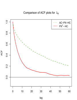
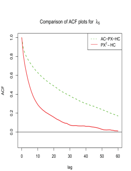
Figure 1: Autocorrelation functions (ACF) for the AC-PX-HC (dashed line) scheme and the proposed $PX^{2}$-HC sampling scheme (solid line), averaged over 100 simulation replicates. The autocorrelation is based on the posteriors of the factor loadings $\lambda_{4}$ (left panel) and $\lambda_{5}$ (right panel) for the two binary phenotypes as simulated in Section 5.1 and described in Table 1.

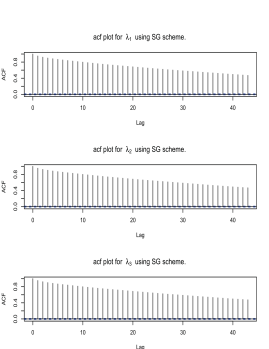
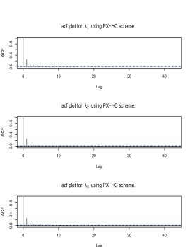
Figure 2: Autocorrelation functions (ACF) for the standard Gibbs (SG) sampling scheme (left panel) and the proposed $PX^{2}$-HC sampling scheme (right panel), averaged over 100 simulation replicates. The autocorrelation is based on the posterior draws for the three factor loadings $\lambda_{j}$s ($j=1,2,3$) for the three continuous phenotypes, as discussed in Section 5.1 and described in Table 1.

Figures 1 and 2 illustrates the significant improvement, in terms of reduced autocorrelation, brought by the additional layer of parameter expansion. See Section 5 for details of the simulations and the Appendix for additional comparison plots.

4 Model and Variable Selection

4.1 Selection of Relevant Phenotypes

In medical research, it is of interest to determine if a phenotype under the study is truly relevant to the latent disease status. In the LVM setting, this is equivalent to testing if the coefficient or factor loading $\lambda_{j}$ for the $j^{th}$ phenotype ((2.1) for continuous phenotype and (2.2) for binary phenotype) is statistically significant or not.

The sign restriction on the factor loadings, $\lambda_{j}s\geq 0$ as discussed in Section 2.2, implies that the highest posterior density interval (HpdI) will seldom include zero and is thus anti-conservative as a selection criterion. To assess the significance of the factor loadings, we apply the Bayesian model selection method using the spike-and-slab priors (Mitchell and Beauchamp, 1988; George and McCulloch, 1993; Chipman, 1996; Xu et al., 2011). Specifically, we use the spike-and-slab prior (3.3) for each $\lambda_{j}^{*}$. The point mass at zero shrinks small values of the factor loading towards zero, while the values of $a$ and $b$ reflect the prior belief in $\lambda_{j}=0$ (see Xu et al., 2011, for a similar discussion on the use of spike-and-slab priors to alleviate the winner’s curse in genetic association studies). When there is no prior information, we recommend $a=1$ and $b=1$ which correspond to $\pi_{j}\sim\text{Unif}(0,1)$. For those phenotypes that are a priori considered to be unrelated to the latent disease variable, we can set $a=0.25$ and $b=1$, thus favouring a priori small values for the corresponding $\lambda_{j}$s.

The determination of the relevance of the $j^{th}$ phenotype is based on the posterior probability of positive loading, $Pr(\lambda_{j}>0|\boldsymbol{Y})$. The sampling algorithm discussed in the Appendix introduces the latent mixture indicator $\omega_{j}=\mathbf{1}_{\{\lambda_{j}>0\}}$, so that $Pr(\lambda_{j}>0|\boldsymbol{Y})$ can be approximated by the MCMC sample frequency of $\{\omega_{j}=1\}$. Given a pre-specified threshold $\phi$, we assume that any loading with $Pr(\lambda_{j}>0|\boldsymbol{Y})\geq\phi$ should be included in the model. The value for $\phi$ depends on the practical problem. If the number of manifest variables is large, the $\phi$ value can be chosen to control the overall average Bayesian false discovery rate (FDR) (Morris et al., 2008). The performance of selecting the correct phenotypes is shown in the simulation Section 5.3.1 below.

4.2 Model Selection Using Bayes Factor

Bayes factors are central to the Bayesian model selection and comparison. The Bayes factor for comparing model $M_{0}$ and $M_{1}$ is defined as: $BF=\frac{P(Y|M_{1})}{P(Y|M_{0})}$. Assuming equal model priors for $M_{0}$ and $M_{1}$, the posterior odds of the two models equals to the Bayes factor. A calibration of the Bayes factor is given by Kass and Raftery (1995) where $\log BF>1$ supports $M_{1}$ and $\log BF<0$ supports $M_{0}$.

The calculation of $P(Y|M_{k})$ in our setting is challenging as it involves high dimensional integration. We follow the procedure of Lee and Song (2002) and use the parametric arithmetic mean path (PAMP) implementation of the path sampling (see also Dutta and Ghosh, 2012) to compute the Bayes factor. Specifically, we assume an unnormalized density function $f_{\theta}$ such that $f_{\theta_{0}}$ and $f_{\theta_{1}}$ are the sampling densities for models $M_{0}$ and $M_{1}$, respectively. The two models are connected in the parametric space $\Theta$ via a path ${\cal{P}}=\{\theta_{g}=g\theta_{0}+(1-g)\theta_{1}:g\in[0,1]\}$, where each $\theta_{g}\in{\cal{P}}$ corresponds to a model $M_{g}$ for which the sampling density function is $f(\theta_{g})$. The Bayes factor can then be calculated using the identity

$$\log BF=\log\frac{P(Y|M_{1})}{P(Y|M0)}=\int_{0}^{1}\!E_{\Omega,\Theta}[{\bf\large U}(Y,\Omega,\Theta,g)]dg,$$ (4.1)

where $E_{\Omega,\Theta}$ denotes the expectation with respect to the density $p(\Omega,\Theta|Y,g)$, and $\mathbf{U}(Y,\Omega,\Theta,g)=\frac{\partial}{\partial g}\log p(Y,\Omega|\Theta,g).$ The dependence of $p(Y,\Omega|\Theta,g)$ on $g$ is due to $p(Y,\Omega|\Theta,g)\propto p(\Omega|Y,\Theta)f_{\theta_{g}}(Y|\Theta)$.

To compute the integral in equation (4.1), we choose $S$ fixed values $\{g_{1},\ldots,g_{S}\}$ such that $g_{(0)}=0<g_{(1)}<g_{(2)}<...<g_{(S)}<1=g_{(S+1)}$ and then estimate $\log BF$ by

$$\widehat{\log BF}=\frac{1}{2}\sum_{s=0}^{S}\!(g_{(s+1)}-g_{(s)})(\overline{{\bf\large U}}_{(s+1)}+\overline{{\bf\large U}}_{(s)}),$$ (4.2)

where $\overline{{\bf\large U}}_{(s)}$ is the average of the values ${\bf\large U}(Y,\Omega,\Theta,g_{(s)})$ over all the MCMC samples from $p(\Omega,\Theta|Y,g_{(s)})$. That is,

$$\overline{{\bf\large U}}_{(s)}=\frac{1}{M}\sum_{k=1}^{M}\!\large U(Y,\Omega^{(k)},\Theta^{(k)},g_{(s)}),$$ (4.3)

in which $\{\Omega^{(k)},\Theta^{(k)};k=1,...,M\}$ are the samples draws from $p(\Omega,\Theta|Y,g_{(s)})$. To estimate $\log BF$, we run the PX$-$HC (or PH${}^{2}-$HC) sampling algorithm for each of the grid points, calculate the values of the parameters and, finally, compute $\overline{\bf\large U}$. This method is also called Path Sampling with Parameter Expansion (PS$-$PX) by Ghosh and Dunson (2009). In the context of pleiotropy studies, Bayes factors can be applied to different hypotheses. In the remaining part of this section we illustrate two instances of substantial interest.

4.2.1 Selection of Relevant Phenotypes via Bayes Factors.

We are concerned here with assessing the factor loadings, $\lambda_{j}$s, as discussed in Section 4.1. Suppose that we are interested in testing $\lambda_{j_{0}}=0$. Let $M_{g}$ be the model with factor loadings equal to $(\lambda_{1},\ldots,\lambda_{j_{0}-1},g\lambda_{j_{0}},\lambda_{j_{0}+1},\ldots,\lambda_{J})^{\prime},$ where $g\in[0,1]$. Thus, model $M_{0}$ has $(\lambda_{1},\ldots,\lambda_{j_{0}-1},0,\lambda_{j_{0}+1},\ldots,\lambda_{J})^{\prime}$, and $M_{1}$ has $(\lambda_{1},\ldots,\lambda_{j_{0}-1},\lambda_{j_{0}},\lambda_{j_{0}+1},\ldots,\lambda_{J})^{\prime}$. The first part of the LVM for $M_{g}$ that links the phenotype $Y_{j}$s and the LV $U$ is

$$\begin{array}[]{cc}V_{citj}=\beta_{0j}+W_{cit}^{T}\beta_{j}+\lambda_{j}U_{cit}+b_{cij}+e_{citj},&\mbox{ if }j\neq j_{0}\\ V_{citj_{0}}=\beta_{0j_{0}}+W_{cit}^{T}\beta_{j_{0}}+g\lambda_{j_{0}}U_{cit}+b_{cij_{0}}+e_{citj_{0}},\\ \end{array}$$ (4.4)

where $V_{citj}=Y_{citj}$ for continuous phenotypes and $V_{citj}=\widetilde{Y}^{b}_{citj}$ for binary phenotypes. The second part of the LVM remains unchanged. We then have

$${\bf\large U}(Y,\Omega,\Theta,g_{(s)})=\frac{1}{\sigma^{2}_{j_{0}}}\sum_{c=1}^{C}\sum_{i=1}^{N_{c}}\sum_{t=1}^{T}\left[V_{citj_{0}}-(\beta_{0j_{0}}+W_{cit}^{T}\beta_{j_{0}}+g_{(s)}\lambda_{j_{0}}U_{cit}+b_{cij_{0}})\right]\lambda_{j_{0}}U_{cit},$$

where $\sigma^{2}_{j_{0}}=1$ for the binary phenotypes. The $logBF$ can then be obtained via Equations (4.2) and (4.3) with $\bf\large U$ calculated using the above equation.

Dutta and Ghosh (2012) showed that the calculation of Bayes factor is valid when $\lim_{g\rightarrow 0}\!E_{\Omega,\Theta}[{\bf\large U}(Y,\Omega,\Theta,g)]$ is finite. The condition holds when the prior distribution for $\lambda$ has the first two moments finite, which is true for our relatively diffuse folded-t prior with ten df. To explore the sensitivity of the Bayes factor estimation to the changes of df in the folded-t prior, we also consider df $\in\{3,10,40,90\}$.

Another concern is the tuning of the grid sizes when using equation (4.2) as the approximation of $\log BF$. Dutta and Ghosh (2012) suggested a grid size no bigger than 0.01, corresponding to 100 grid numbers in $[0,1]$. However, due to conflict between the prior and sampling distributions, when $\lambda$ is large, $E_{\Omega,\Theta}[{\bf\large U}(Y,\Omega,\Theta,g)]$ has large spikes when $g$ is close to zero, but it stabilizes gradually as $g$ increases. Thus we suggest to use uneven grid size scheme so that smaller grid sizes are chosen for $g$ near zero. For example, in our simulations below we set the grid number to be 15 for $g\in[0,0.1]$ and also 15 for $g\in[0.9,1]$ and observed good results.

4.2.2 Selection of Pleiotropic Genetic Marker via Bayes Factors

An important inferential focus in genetic pleiotropy study is the selection of genetic marker(s) with pleiotropic effect. Particularly, we are interested in testing the effect of a genetic marker on the LV. Suppose that the fixed-effect covariates $X$ in the second part of the LVM has two components where $X_{1}$ is the set of clinical covariates and $X_{2}$ is the genotype of the marker of interest. The two competing LV models are then

$$M_{0}:\left\{\begin{array}[]{ll}y^{c}_{citj}=\beta_{0j}+W_{cit}^{T}\beta_{j}+\lambda_{j}U_{cit}+b_{cij}+e_{citj},&j=1,...,J_{1},\\ \widetilde{y}^{b}_{citj}=\beta_{0j}+W_{cit}^{T}\beta_{j}+\lambda_{j}U_{cit}+b_{cij}+e_{citj},&j=J_{1}+1,...,J,\\ U_{cit}=X_{1_{cit}}^{T}\alpha_{1}+Z_{cit}^{T}a_{c}+Q_{cit}^{T}d_{ci}.&\\ \end{array}\right.$$

$$M_{1}:\left\{\begin{array}[]{ll}y^{c}_{citj}=\beta_{0j}+W_{cit}^{T}\beta_{j}+\lambda_{j}U_{cit}+b_{cij}+e_{citj},&j=1,...,J_{1},\\ \widetilde{y}^{b}_{citj}=\beta_{0j}+W_{cit}^{T}\beta_{j}+\lambda_{j}U_{cit}+b_{cij}+e_{citj},&j=J_{1}+1,...,J,\\ U_{cit}=X_{1_{cit}}^{T}\alpha_{1}+X_{2_{cit}}^{T}\alpha_{2}+Z_{cit}^{T}a_{c}+Q_{cit}^{T}d_{ci}.&\\ \end{array}\right.$$

The two models can be linked up by the parameter $g\in[0,1]$ as:

$$M_{g}:\left\{\begin{array}[]{ll}y^{c}_{citj}=\beta_{0j}+W_{cit}^{T}\beta_{j}+\lambda_{j}U_{cit}+b_{cij}+e_{citj},&j=1,...,J_{1},\\ \widetilde{y}^{b}_{citj}=\beta_{0j}+W_{cit}^{T}\beta_{j}+\lambda_{j}U_{cit}+b_{cij}+e_{citj},&j=J_{1}+1,...,J,\\ U_{cit}=X_{1_{cit}}^{T}\alpha_{1}+gX_{2_{cit}}^{T}\alpha_{2}+Z_{cit}^{T}a_{c}+Q_{cit}^{T}d_{ci}.&\\ \end{array}\right.$$

Let $L_{g}$ be the complete-data likelihood for model $M_{g}$, then

$${\bf\large U}(Y,\Omega,\Theta,g_{(s)})=\frac{\partial\log L_{g}}{\partial g}=\sum_{c=1}^{C}\sum_{i=1}^{N_{c}}\sum_{t=1}^{T}\left(U_{cit}-X_{1_{cit}}^{T}\alpha_{1}-g_{(s)}X_{2_{cit}}^{T}\alpha_{2}-Z_{cit}^{T}a_{c}-Q_{cit}^{T}d_{ci}\right)X_{2_{cit}}^{T}\alpha_{2}.$$

Again $\log BF$ can be obtained using (4.2) and (4.3) with $\bf\large U$ calculated as above.

5 Simulation study

We have identified three practically relevant issues related to the model’s performance that we wanted to study via simulations: 1) the performance of our proposed method in parameter estimation, 2) the effect of ignoring the family structure, and 3) the performance of the proposed variable selection methods introduced in Section 4.

Table 1 provides the details of the simulation models in terms of phenotype $Y$ and covariates $W$ and $X$ specifications. Without loss of the generality, in all simulations we assume that there are 500 families/clusters, each contributing 1, 2, 3, 4 or 5 siblings with probability, respectively, 0.3, 0.4, 0.2, 0.07 and 0.03. To simulate the genotypes for the siblings, we set the minor allele frequency (MAF) to be 0.1, and we assume that the parental genotypes for the 500 families follow Hardy Weinberg equilibrium(HWE). The siblings’ genotypes are then obtained by using Mendel’s first law of segregation. The parental genotypes however are not used for the analysis because they are often not available in practical settings. Continuous covariates are assumed to follow a $N(0,1)$ distribution with correlation coefficient within the family (familial correlation) being 0.3 and individual-specific trajectories for the covariate (serial correlation) follow an AR(1) model with autocorrelation being 0.3. We also assume that each phenotype is measured over time five times. Unless specified otherwise, the default choice is $\pi_{j}\sim\text{Beta}(1,1)$ in the spike-and-slab prior given in (3.3), assuming no prior information on the relationship between phenotype $j$ and the LV. In all the simulations, we run the MCMC algorithm for 25,000 iterations, discarding the first 5,000 samples as burn-in.

5.1 Parameter estimation for general traits.

To evaluate the performance of the proposed parameter estimation, we assume here that five phenotypes are of interest among which $y_{1}$, $y_{2}$ and $y_{3}$ are continuous, and $y_{4}$ and $y_{5}$ are binary (Tables 1 and 2). We use a total of 100 replications to study the variation of estimates and also compare the performance of our PX${}^{2}-$HC algorithm with those of the standard algorithms.

Figure 1 shows that, compared to AC-PX-HC, the standard PX algorithm with the DA scheme of Albert and Chib (1993), the proposed PX${}^{2}-$HC algorithm drastically reduces the autocorrelations between the chains’s realizations which implies an increase in Monte Carlo efficiency. The improvement is also evident in Figure 2, when comparing the standard Gibbs (left column) with the proposed PX${}^{2}-$HC scheme (right plots). In the Appendix, we provide the corresponding trace plots to illustrate the improved mixing of the PX${}^{2}-$HC chain.

Table 2 shows the true values, mean estimates and root mean square errors (RMSE) for all the parameters in the model. Results show that the estimates have good accuracy with small bias and RMSE. However, parameter estimation for binary responses is less accurate than for continuous phenotypes, which is not surprising given the discrepancy between the information provided by the two types of data.

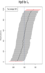
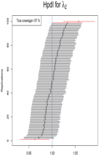
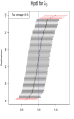
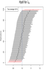
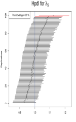
Figure 3: The 95% highest posterior density intervals (HpdI) for each of the five factor loadings $\lambda_{j}$s. The HpdI from the 100 simulation replicates are ordered by the lower bounds of the intervals. The vertical line is the true value and “X” marks the estimate from each simulation replicate. The red HpdI do not cover the true value. The empirical coverages of the HpdI are 94%, 95%, 91%, 94%, 95% (from left to right), respectively, for the five phenotypes $y_{1}$, $y_{2}$, $y_{3}$, $y_{4}$ and $y_{5}$ as simulated in Section 5.1 and described in Table 1. The legend indicates the empirical coverage estimated from the 100 intervals.

Figure 3 shows that around $95\%$ of the HpdIs for the factor loadings $\lambda$s cover the true values. However, this remains to be validated theoretically for more general setting as results seem to suggest a matching prior type of result.

5.2 Effect of Ignoring Family Structure

In this simulation, we only consider the three continuous phenotypes $y_{1}$, $y_{2}$ and $y_{3}$ and generate data with familial and serial correlations as above in Section 5.1. We compare parameter estimates obtained using the proposed method to model the familial correlation with the estimates obtained using the method of Roy and Lin (2000) assuming samples are independent of each other.

The simulation results in Table 3 show that failure to account for the familial correlation present in the data will not only yield incorrect conclusion of the serial correlations between phenotypes $\Sigma_{D}$, but also cause over-estimation of the factor loading $\lambda_{j}$, which quantifies the strength of the relationship between phenotype $y_{j}$ and the latent variable $U$, and under-estimation of $\alpha_{1}$ and $\alpha_{2}$, which respectively, represents the effect of the clinical covariate and genetic marker on $U$.

5.3 Model and Variable Selection

5.3.1 Selection of Relevant Phenotypes via Spike-and-Slab Priors

To assess the performance of phenotype selection using the spike-and-slab prior (3.3) as described in Section 4.1, we consider here four continuous phenotypes $y^{c}$ with factor loading $\lambda_{j}$s being set to $(0.5,0.05,0.02,0)$ and three binary phenotypes $y^{b}$ with $\lambda_{j}$s being $(0.2,0.01,0)$. We chose these values so that the strength of the association between a phenotype and the LV $U$ ranges from strong ($\lambda_{j}=0.5$) to no association ($\lambda_{j}=0$). We set $\pi\sim\text{Beta}(0.25,1)$ which favours a priori the null ($\lambda_{j}=0$). After the calculation of the posterior frequency of $\omega_{j}=1$ for each phenotype in the 100 replicates, a threshold of $\phi=50\%$ is used on the posterior probability $Pr(\lambda_{j}>0|\boldsymbol{Y})$.

Simulation results show that the type I error of this selection procedure is about 5% in that, for the phenotype not associated with the latent disease status ($\lambda_{j}=0$), around 5% of the replications have $Pr(\lambda_{j}>0|\boldsymbol{Y})\geq 0.5$. For phenotypes moderately or strongly associated the latent variable ($\lambda_{j}=0.05$ or higher), we have 100% power of making the correct decision. However, power is reduced for weakly associated phenotypes as expected. Specifically for the case consider here, power is 71% for the phenotype with $\lambda_{j}=0.02$ and 16% for $\lambda_{j}=0.01$.

5.3.2 Selection of Relevant Phenotypes via Bayes Factors

We have also examined the performance of phenotype selection via Bayes factors for the comparison of model $M_{1}$ (assuming $\lambda>0$) and model $M_{0}$ (assuming $\lambda=0$) using the same simulation model as in the previous section. The $logBF$s for the $\lambda$’s are calculated using the folded-t prior with df $=10$ as described in Section 4.2.1.

Results in Table 4 show that when phenotype $y_{j}$ is truly associated with the latent variable with $\lambda_{j}\geq 0.05$, the average estimated $log(BF)>5.9$. This and combined with the SD shown in the table suggest that, for such cases, the Bayes factor criterion chooses the correct alternative model $100\%$ of the times. When phenotype $y_{j}$ is truly not associated with the LV ($\lambda_{j}=0$), the Bayes factor criterion correctly favors the null model with the average estimated $log(BF)<-2.4$. However, the Bayes factor criterion has little ability in identifying weakly associated phenotypes ($\lambda_{j}\leq 0.02$), which is inferior to the spike-and-slab approach in the previous section. We have also explored the use of other folded-t priors with df ranging from 3, 10, 40 to 90. We find that all the prior settings give us the same conclusion on the model selection.

5.3.3 Selection of Pleiotropic Genetic Marker or Other Covariates

For this purpose, we assume that there are five indirect fixed-effect covariates $X_{1},\ldots,X_{5}$ in the second part of the LVM that models the effect of the genetic marker and other covariates on the latent variable. We assume that $X_{3}$ is the genotype of the marker of interest and the remaining ones are standardized continuous variables. Coefficients $(\alpha_{1},\alpha_{2},\alpha_{3},\alpha_{4},\alpha_{5})$ quantify the effects of the five covariates which are set to be $(1.0,-0.5,0.2,0,0)$. We also assume that there are two continuous standardized direct fixed-effect covariates $W_{1}$ and $W_{2}$ in the first part of the LVM with effects ($\beta_{1}=0.5$ and $\beta_{2}=0.3$) on all the phenotypes.

Table 5 shows the estimated $log(BF)$ for comparing the null model assuming $\alpha_{j}=0$ with the alternative of association. The prior distribution for $\alpha$ in (2.4) is $\alpha\sim N(0,\mathbf{I}_{5})$. Results show that the proposed Bayes factor criterion has the ability to detect the association between the genetic marker and the latent variable, therefore pleiotropy, with the average estimated $log(BF)=6.3$ and SD $=2.39$. The Bayes factor variable selection criterion also has good result for the two associated covariates $X_{1}$ and $X_{2}$ for which the average $log(BF)$ estimate is, respectively, 337.5 and 6.3, as well as for the two covariates $X_{4}$ and $X_{5}$ with zero effect, for which the estimated $log(BF)$ is consistently less than $-1.9$ with SD $=0.42$.

6 Application to a genetic study of type 1 diabetes (T1D) complications.

Here we demonstrate the practical utility of the proposed LVM method by investigating the blood pressure data from a genome-wide association study (GAWS) of various T1D complications (Paterson et al., 2010). The study sample consists of $n=1300$ individuals with T1D from the Diabetes Control and Complications Trial (DCCT). Various phenotypes thought be to related to T1D complication severity, including glycosylated hemoglobin (HbA1c) and diastolic (DBP) and systolic blood pressure (SBP), were collected from each subject over the course of the DCCT. Additional covariates such as sex and body mass index (BMI) were also collected, and individuals were from two different cohorts and subjected to two treatment types (conventional vs. intensive). Over 800K SNPs were genotyped by the Illumina 1M bead chip assay for these individuals.

Because T1D is a complex disease with various complication measures (the observed phenotypes), it is of great interest to quantify the conceptual latent complication status, as well as to understand the influencing factors (both genetic markers and clinical covariates). In addition, it is valuable to determine if the various observed phenotypes are truly associated with the latent variable. However, due to lack of suitable statistical methodology, previous analyses have been limited to the standard uni-phenotype approach, analyzing one phenotype at a time. For example, Ye et al. (2010) recently performed GAWS, separately, for DBP and SBP, and they identified rs7842868 on chromosome 8 as a SNP significantly associated with DBP.

Our goal here is to formally perform a multi-phenotype analysis, jointly analyzing DBP and SBP using the proposed Bayesian LVM methodology. This approach allows us not only to determine if rs7842868 is associated with the latent conceptual T1D complication variable, but also to test if DBP and SBP are truly related to the LV. It is also of practical interest to study whether there are other phenotypes such as hyperglycemia (HPG) influence the latent complication severity variable.

In our application, we investigate three phenotypes $Y$ among which two are continuous (DBP and SBP) and one is binary (HPG $=1$ for hyperglycemia if and $=0$ for normal glycemia), all are longitudinal. Hyperglycemia at a given time point is defined if the corresponding HbA1c is greater or equal to 8. Among the available covariates, based on suggestions from clinicians, covariates $W$ that have direct effects on the phenotypes include BMI, and covariates $X$ that have direct effects on the LV include sex, cohort and treatment. Among the 10 longitudinal measurements available, there are significant amount of missing data after the $7^{th}$ measure (due to staggered entry) while there are little missing data before the $5^{th}$ measure. Therefore, we only use the first five measurements. We treat the remaining missing data as Missing at Random (MAR), and we replace the missing data with the means of all the other measurements. In this dataset, there is only one person in each family therefore there is no familial correlation, but the proposed methodology remains suitable by assuming the cluster size being 1.

We first consider rs7842868, a SNP found by Ye et al. (2010) to be associated with DBP. In this case $X_{1}$ is the genotype of rs7842868. Results in Table 6 show that DBP and SBP are clearly associated with the latent variable with estimated $logBF$ over 100, while HPG is not. We also applied the spike-and-slab prior method for phenotype selection as discussed in Sections 4.1 and 5.3.1, the poster probability $Pr(\lambda_{j}>0|\boldsymbol{Y})$ is 1 for DBP and SBP and 0.235 for HPG. Thus all model selection criteria consistently suggest that both DBP and SBP are significantly related to the latent variable but not HPG. Results also show that SNP rs7842868 is significantly associated with the latent variable with estimated $logBF$ over 10 and the 95% HpdI not covering 0. The sign of the effect suggest that the minor allele of the SNP is protective in that it decreases the latent complication severity score. The combined evidence from both parts of the LVM show that rs7842868 has pleiotropic effect on the two blood pressures. Sex and cohort are also found to be significantly associated with the latent variable but not treatment.

We then investigate rs1358030, a SNP found by Paterson et al. (2010) to be associated with HbA1c. In this case, $X_{1}$ is the genotype of rs1358030. Based on results in Table 6, there is no evidence that rs1358030 is significantly associated with the latent variable. Our application here considers the binary hyperglycaemia (HPG) as the third phenotype of interest instead of the continuous HbA1c variable. Besides clinical consideration, this choice also allows us to evaluate the proposed method for general traits as described in Section 3.2.2

To further evaluate the proposed method, we simulate genotypes for two NULL SNPs that are not associated with the phenotypes of interest. One SNP has MAF equal to 0.25, the MAF of rs7842868), and the other one has MAF equal to 0.35, the MAF of rs1358030. As expected, no significant associations are detected.

7 Conclusion and Disucssion

We propose here a Bayesian latent variable approach to joint model multiple outcomes, motivated by genetic association studies of pleiotropic effects. The method can handle continuous and binary responses while accounting for serial and familial correlation structures in the data. The postulated latent variable represents the underlying severity or complication level of a trait and characterizes the totality of multiple observed phenotypes of interest. If additional phenotypes were to be measured, the latent variable could change its significance since it would encapsulate a richer set of manifest variables. The central feature of the model is that it allows us to consider the strength of dependence between the genotype and each of the phenotypes in a unified manner. The Bayesian approach takes into account all the uncertainty present in the model and incorporates prior information if available. The computational challenges are met via the use of parametric expansion techniques.

An important issue for pleiotropy studies is the assessment of importance of each variable. We have adopted two Bayesian techniques that are shown to be effective in variable selection. We found that both Bayes factor and spike-and-slab prior perform well with the latter slightly more efficient in terms of detecting weak signals.

Our proof-of-principle application to a genetic study of type 1 diabetes complications demonstrates the utility of the method in a real data setting. So far, genetic association studies of various T1D complication-related measures have been limited to studying one phenotype at a time. The proposed method jointly analyzes two continuous and one binary phenotypes of interest, and it provides evidence for the association between the phenotypes and the latent severity of T1D complication, the association between the latent variable and genetic markers of interest, and the effect of other covariates on the phenotypes and the latent variable.

The computational load in the current implementation of the proposed method makes it impractical to perform a genome-wide search for pleiotropic genetic variants. The recent advances in parallel computing can partially alleviate this constraint. Alternatively, a two-stage approach can be used in which a simple and less stringent selection procedure is first used to select a moderate number of candidate variants for further investigation using the proposed method. The uncertainty inherited from the first-stage selection, however, must be accounted for in the models used in the second stage.

Table 1: Simulation and Application Models

	Simulation Model Considered in				Application Model
	Section 5.1	Section 5.2	Sections 5.3.1&5.3.2	Section 5.3.3	Section 6
Phenotypes of interest
$y_{1}$	$\surd$ (continuous)	$\surd$ (continuous)	$\surd$ (continuous)	$\surd$ (continuous)	SBP (continuous)
$y_{2}$	$\surd$ (continuous)	$\surd$ (continuous)	$\surd$ (continuous)	$\surd$ (continuous)	DBP (continuous)
$y_{3}$	$\surd$ (continuous)	$\surd$ (continuous)	$\surd$ (continuous)	$\surd$ (continuous)	HPG (binary)
$y_{4}$	$\surd$ (binary)		$\surd$ (continuous)	$\surd$ (binary)
$y_{5}$	$\surd$ (binary)		$\surd$ (binary)	$\surd$ (binary)
$y_{6}$			$\surd$ (binary)
$y_{7}$			$\surd$ (binary)
Covariates with direct effect $\boldsymbol{\beta}$ on $Y$
$W_{1}$	$\surd$ (continuous)	$\surd$ (continuous)	$\surd$ (continuous)	$\surd$ (continuous)	BMI
$W_{2}$				$\surd$ (continuous)
Covariate with indirect effect on $Y$ but with direct effect $\boldsymbol{\alpha}$ on the latent variable $U$
$X_{1}$	$\surd$ (continuous)	$\surd$ (continuous)	$\surd$ (continuous)	$\surd$ (continuous)	genotype
$X_{2}$	$\surd$ (genotype)	$\surd$ (genotype)	$\surd$ (genotype)	$\surd$ (continuous)	sex
$X_{3}$				$\surd$ (genotype)	cohort
$X_{4}$				$\surd$ (continuous)	treatment
$X_{5}$				$\surd$ (continuous)
Latent variable $U$ has direct effect $\boldsymbol{\lambda}$ (also called factor loading) on each of the $Y$s

Table 2: Performance of the proposed parameter estimation method. First three phenotypes $y_{1}$, $y_{2}$ and $y_{3}$ are continuous and the last two phenotypes $y_{4}$ and $y_{5}$ are binary. Results are based on 100 replicates that were simulated as described in Section 5.1 and Table 1.

First part of the latent variable model
Parameter	True value	Estimate	RMSE
$\lambda_{j}$, the factor loading for phenotype $y_{j}$ and the latent variable $U$
$\lambda_{1}$	1.0	1.000	0.007
$\lambda_{2}$	1.0	1.000	0.007
$\lambda_{3}$	1.0	1.000	0.007
$\lambda_{4}$	1.0	1.000	0.022
$\lambda_{5}$	1.0	0.998	0.025
$\beta_{j}$ for phenotype $y_{j}$ and covariate $W$
$\beta_{1}$	1.0	1.000	0.011
$\beta_{2}$	1.0	1.000	0.011
$\beta_{3}$	1.0	1.000	0.011
$\beta_{4}$	1.0	1.005	0.026
$\beta_{5}$	1.0	0.996	0.031
Second part of the latent variable model
Parameter	True value	Estimate	RMSE
$\alpha$ for the latent variable $U$ and covariates ($\alpha_{2}$ for the genetic marker $X_{2}$)
$\alpha_{1}$	1.0	0.999	0.011
$\alpha_{2}$	1.0	1.011	0.074
Correlation parameters
Parameter	True value	Estimate	RMSE
$\tau_{1}^{2}$	0.2	0.200	0.014
$\tau_{2}^{2}$	0.2	0.201	0.012
$\tau_{3}^{2}$	0.2	0.200	0.013
$\tau_{4}^{2}$	0.2	0.202	0.033
$\tau_{5}^{2}$	0.2	0.200	0.032
$\Sigma_{A}$	0.5	0.519	0.046
$\Sigma_{D}$	0.3	0.320	0.032

Table 3: Effect of ignoring familial correlation present in the data. Results are the averages over 100 simulation replications. The coefficient $\alpha_{2}$ evaluates the effect of a genetic marker on the latent variable $U$ ($\alpha_{1}$ for a clinical covariate on $U$), and $\lambda_{j}$s evaluate the effect of $U$ on the three phenotypes of interest. Details of the simulations are in Section 5.2 and Table 1.

			With Familial Corr.			Without Familial Corr.
Parameters		True Value	Bias	SD	RMSE	Bias	SD	RMSE
$\beta$	$\beta_{1}$	1.0	-0.002	0.018	0.019	-0.003	0.028	0.027
	$\beta_{2}$	1.0	-0.001	0.020	$0.019$	-0.002	0.024	0.028
	$\beta_{3}$	1.0	-0.002	0.019	$0.019$	-0.003	0.027	0.028
$\alpha$	$\alpha_{1}$	1.0	0.009	0.074	0.075	-0.233	0.099	0.235
	$\alpha_{2}$	1.0	0.009	0.020	0.021	-0.227	0.028	0.244
$\lambda$	$\lambda_{1}$	1.0	-0.009	0.014	0.015	0.308	0.029	0.310
	$\lambda_{2}$	1.0	-0.009	0.014	0.016	0.308	0.028	0.309
	$\lambda_{3}$	1.0	-0.009	0.015	0.015	0.308	0.029	0.309
$\tau^{2}$	$\tau^{2}_{1}$	0.2	-0.002	0.013	0.015	-0.001	0.015	0.015
	$\tau^{2}_{2}$	0.2	-0.001	0.012	0.014	-0.001	0.013	0.015
	$\tau^{2}_{3}$	0.2	-0.002	0.012	0.013	0.000	0.014	0.014
$\sigma^{2}$	$\sigma^{2}_{1}$	0.1	0.002	0.004	0.004	0.002	0.004	0.004
	$\sigma^{2}_{2}$	0.1	0.001	0.004	0.004	0.001	0.004	0.004
	$\sigma^{2}_{3}$	0.1	0.002	0.004	0.004	0.002	0.004	0.004
$\Sigma_{A}$	$(\Sigma_{A})_{11}$	1.0	-0.003	0.08	0.089	N/A	N/A	N/A
	$(\Sigma_{A})_{12}$	0.0	0.004	0.06	0.064	N/A	N/A	N/A
	$(\Sigma_{A})_{22}$	1.0	0.034	0.08	0.085	N/A	N/A	N/A
$\Sigma_{D}$	$(\Sigma_{D})_{11}$	0.1	0.049	0.020	0.053	0.69	0.06	0.696
	$(\Sigma_{D})_{12}$	0.0	0.000	0.011	0.011	-0.002	0.022	0.023
	$(\Sigma_{D})_{22}$	0.1	0.029	0.023	0.033	0.047	0.021	0.052

Table 4: The estimated $logBF$ for testing the factor loading $\lambda_{j}$. $\lambda_{j}$ quantifies the association between phenotype $y_{j}$ and the latent variable. Results are based on 50 simulated replicates. Details of the simulations are in Section 5.3.2 and Table 1.

	Continuous Phenotypes				Binary Phenotypes
	$y_{1}$	$y_{2}$	$y_{3}$	$y_{4}$	$y_{5}$	$y_{6}$	$y_{7}$
True $\lambda_{j}$	0.5	0.05	0.02	0	0.2	0.01	0
$\widehat{logBF}$	121.60	5.91	-1.76	-2.67	22.11	-2.43	-2.43
SD	6.47	2.22	1.05	0.47	8.19	0.32	0.13

Table 5: The estimated $logBF$ for testing $\alpha=0$. $\alpha$ quantifies the association between the covariates and the latent variable. Results are based on 50 simulated replicates. Details of the simulations are in Section 5.3.3 and Table 1.

	Covariates with effect on the latent variable
	$X_{1}$	$X_{2}$	$X_{3}$ (genotype)	$X_{4}$	$X_{5}$
True $\alpha$	1.0	-0.5	0.2	0	0
$\widehat{logBF}$	337.53	94.99	6.30	-1.94	-1.95
SD	33.25	11.19	2.39	0.46	0.42

Table 6: Application results. SNP rs7842868 was previously identified to be associated with diastolic blood pressure (DBP) and SNP rs1358030 was previously identified to be associated with HbA1c. Phenotypes of interest are DBP and systolic blood pressure (SBP), two continuous outcomes, and hyperglycemia (HPG, defined as HbA1c greater or equal to 8), a binary outcome. All phenotypes are thought to be related to type 1 diabetes complication severity. The coefficient $\lambda$s assess the association between the phenotypes and the latent T1D complication status, and $\alpha$s evaluate the association between the latent variable and the genetic marker and the other covariates of interest. See Section 6 and Table 1 for more details.

Analysis of SNP rs7842868
	Parameter	Estimate	95% HpdI	$\widehat{logBF}$
SBP	$\lambda_{1}$	6.621	(6.153, 7.077)	114.85
DBP	$\lambda_{2}$	3.842	(3.566, 4.110)	112.98
HPG	$\lambda_{3}$	0.011	($2.189\times 10^{-7}$, $2.975\times 10^{-2}$)	-1.05
rs7842868	$\alpha_{1}$	-0.269	(-0.372, -0.164)	10.06
sex	$\alpha_{2}$	-0.721	(-0.866, -0.584)	62.27
cohort	$\alpha_{3}$	0.443	( 0.299, 0.585)	20.15
treatment	$\alpha_{4}$	0.128	(-0.004, 0.263)	0.366
Analysis of SNP rs1358030
	Parameter	Estimate	95% HpdI	$\widehat{logBF}$
SBP	$\lambda_{1}$	6.868	(6.439, 7.302)	128.3
DBP	$\lambda_{2}$	3.706	(3.491, 3.933)	120.2
HPG	$\lambda_{3}$	0.010	($2.566\times 10^{-7}$, $2.740\times 10^{-7}$)	-1.034
rs1358030	$\alpha_{1}$	- 0.039	(-0.049, 0.122)	-1.104
sex	$\alpha_{2}$	-0.758	(-0.880, -0.623)	64.86
cohort	$\alpha_{3}$	0.393	(0.258, 0.532)	18.17
treatment	$\alpha_{4}$	0.088	(-0.041, 0.220)	-0.18

References

- Albert and Chib (1993) Albert, J. and Chib, S. (1993). Bayesian analysis of binary and polychotomous response data. Journal of the American Statistical Association 88 669–679.
- Bartholomew et al. (2011) Bartholomew, D., Knott, M. and Moustaki, I. (2011). Latent Variable Models and Factor Analysis: A Unified Approach. Wiley Series in Probability and Statistics, John Wiley & Sons, Ltd.
- Burton et al. (2005) Burton, P., Scurrah, K., MD.Tobin and Palmer, L. (2005). Covariance components models for longitudinal family data. International Journal of Epidemiology 34 1063–1067.
- Chipman (1996) Chipman, H. (1996). Bayesian variable selection with related predictors. Canad. J. Statist. 24 17–36.
- Dutta and Ghosh (2012) Dutta, R. and Ghosh, J. K. (2012). Bayesian model selection with path sampling: factor models and other examples. Statistical Science. (to appear) .
- Gelfand (1995) Gelfand, A. E. (1995). Efficient parametrisations for normal linear mixed models. Biometrika 82 479–488.
- Gelman (2006) Gelman, A. (2006). Prior distributions for variance parameters in hierarchical models. Bayesian Analysis 1 515–533.
- George and McCulloch (1993) George, E. I. and McCulloch, R. E. (1993). Variable selection via Gibbs sampling. J. Amer. Statist. Assoc. 88 881–889.
- Ghosh and Dunson (2009) Ghosh, J. and Dunson, D. B. (2009). Default prior distributions and efficient posterior computation in bayesian factor analysis. Journal of Computational and Graphical Statistics 18(2) 306–320.
- Jöreskog and Sörbom (1996) Jöreskog, K. and Sörbom, D. (1996). LISREL8: User’s Reference Guide. Scientific Software International, Inc.
- Kass and Raftery (1995) Kass, R. E. and Raftery, A. E. (1995). Bayes factors. Journal of the American Statistical Association 90 773–795.
- Lange and Whittaker (2001) Lange, C. and Whittaker, J. C. (2001). Mapping quantitative trait loci using generalized estimating equations. Genetics 159 1325–1337.
- Lee and Song (2002) Lee, S. Y. and Song, X. Y. (2002). Bayesian selection on the number of factors in a factor analysis model. Behaviormetrika 29 23–40.
- Liu and Wu (1999) Liu, J. S. and Wu, Y. N. (1999). Parameter expansion for data augmentation. Journal of the American Statistical Association 94 1264–1274.
- Meng and van Dyk (1999) Meng, X.-L. and van Dyk, D. (1999). Seeking efficient data augmentation schemes via conditional and marginal augmentation. Biometrika 86 301–320.
- Mitchell and Beauchamp (1988) Mitchell, T. and Beauchamp, J. (1988). Bayesian variable selection in linear regression, (with discussion). J. Am. Stat. Assoc. 83 1023–1032.
- Morris et al. (2008) Morris, J. S., Brown, P. J., Herrick, R. C., Beggerly, K. A. and Coombes, K. R. (2008). Bayesian analysis of mass spectrometry data using wavelet-based functional mixed models. Biometrics. 64 479–489.
- Muthen and Asparouhov (2011) Muthen, B. and Asparouhov, T. (2011). Beyond multilevel regression modeling: Multilevel analysis in a general latent variable framework. In J. Hox and J.K. Roberts (eds), Handbook of Advanced Multilevel Analysis. New York: Taylor and Francis.
- Nock et al. (2009) Nock, N. L., Wang, X., Thompson, C. L., Song, Y., Baechle, D., Raska, P., Stein, C. M. and Gray-McGuire1, C. (2009). Defining genetic determinants of the metabolic syndrome in the framingham heart study using association and structural equation modeling methods. BMC Proceedings 3.
- O’Hara et al. (2010) O’Hara, R. B., Komulainen, P., Savolainen, O. and Sillanpaa, M. J. (2010). A latent variable approach to multivariate quantitative trait loci. Nature Precedings .
- Paterson et al. (2010) Paterson, A. D., Waggott, D. and et al., A. P. B. (2010). A genome-wide association study identifies a novel major locus for glycemic control in type 1 diabetes, as measured by both a1c and glucose. Diabetes 59 539–549.
- Roy and Lin (2000) Roy, J. and Lin, X. (2000). Latent variable models for longitudinal data with multiple continuous outcomes. Biometrics 56 1047–1054.
- Sammel and Ryan (1996) Sammel, M. D. and Ryan, L. M. (1996). Latent variable models with fixed effects. Biometrics 52 650–663.
- Sammel and Ryan (1997) Sammel, M. D. and Ryan, L. M. (1997). Latent variable models for mixed discrete and continuous outcomes. Journal of the Royal Statistical Society. Series B 59 667–678.
- Tanner and Wong (1987) Tanner, M. and Wong, W. (1987). The calculation of posterior distributions by data augmentation. J. Amer. Statist. Assoc. 82 528–540.
- Tayo et al. (2008) Tayo, B., Harders, R., Luke, A., Zhu, X. and Cooper, R. (2008). Latent common genetic components of obesity traits. International Journal of Obesity 32 1799–1806.
- Thornton and McPeek (2010) Thornton, T. and McPeek, M. S. (2010). Roadtrips: Case-control association testing with partially or completely unknown population and pedigree structure. The American Journal of Human Genetics 86 172–184.
- van Dyk and Meng (2001) van Dyk, D. A. and Meng, X.-L. (2001). The art of data augmentation. Journal of Computational and Graphical Statistics 10 1–50.
- Weller et al. (1996) Weller, J. I., Wiggans, G. R., VanRaden, P. M. and Ron, M. (1996). Application of canonical transformation to detection of quantitative trait loci with the aid of genetic markers in a multitrait experiment. Theoretical and Applied Genetics 92 998–1002.
- Xu et al. (2011) Xu, L., Craiu, R. V. and Sun, L. (2011). Bayesian methods to overcome the winner’s curse in genetic studies. The Annals of Applied Statistics 5 201–231.
- Xu et al. (2003) Xu, X., Lu, T. and Wei, L. J. (2003). Combining dependent tests for linkage or association across multiple phenotypic traits. Biostatistics 4 223–229.
- Ye et al. (2010) Ye, C., Canty, A. J., Waggott, D., Sylvestre, M.-P., Shen, E., Hosseini, M. and et al. (2010). A repeated measures genome wide association study of blood pressure in type 1 diabetes. abstract # 203 presented at the nineteenth annual meeting of the international genetic epidemiology society. Genetic Epidemiology 34 973.