The Collisional Evolution of Debris Disks

Abstract

We explore the collisional decay of disk mass and infrared emission in debris disks. With models, we show that the rate of the decay varies throughout the evolution of the disks, increasing its rate up to a certain point, which is followed by a leveling off to a slower value. The total disk mass falls off $\propto t^{-0.35}$ at its fastest point (where $t$ is time) for our reference model, while the dust mass and its proxy – the infrared excess emission – fades significantly faster ($\propto t^{-0.8}$). These later level off to a decay rate of $M_{\rm tot}(t)\propto t^{-0.08}$ and $M_{\rm dust}(t)~{}{\rm or}~{}L_{\rm ir}(t)\propto t^{-0.6}$. This is slower than the $\propto t^{-1}$ decay given for all three system parameters by traditional analytic models.

We also compile an extensive catalog of Spitzer and Herschel 24, 70, and 100 $\micron$ observations. Assuming a log-normal distribution of initial disk masses, we generate model population decay curves for the fraction of stars harboring debris disks detected at 24 $\mu$m. We also model the distribution of measured excesses at the far-IR wavelengths (70–100 $\micron$) at certain age regimes. We show general agreement at 24 $\micron$ between the decay of our numerical collisional population synthesis model and observations up to a Gyr. We associate offsets above a Gyr to stochastic events in a few select systems. We cannot fit the decay in the far infrared convincingly with grain strength properties appropriate for silicates, but those of water ice give fits more consistent with the observations (other relatively weak grain materials would presumably also be successful). The oldest disks have a higher incidence of large excesses than predicted by the model; again, a plausible explanation is very late phases of high dynamical activity around a small number of stars.

Finally, we constrain the variables of our numerical model by comparing the evolutionary trends generated from the exploration of the full parameter space to observations. Amongst other results, we show that erosive collisions are dominant in setting the timescale of the evolution and that planetesimals on the order of 100 km in diameter are necessary in the cascades for our population synthesis models to reproduce the observations.

1. Introduction

Planetary debris disks provide the most accessible means to explore the outer zones of planetary systems over their entire age range – from 10 Gyr to examples just emerging from the formation of the star and its planets at 10 Myr. Debris disks are circumstellar rings of dust, rocks, and planetesimals, which become visible in scattered light and infrared emission because of their large surface areas of dust. Because this dust clears quickly, it must be constantly replenished through collisions amongst the larger bodies, initiated by the dynamical perturbing forces of nearby planets (Wyatt, 2008). Thus, the presence of a debris disk signals not only that the star has a large population of planetesimals, but that there is possibly at least one larger body to stir this population (Kenyon & Bromley, 2001; Mustill & Wyatt, 2009; Kennedy & Wyatt, 2010). The overall structures of these systems are indicative of the processes expected to influence the structures of the planetary systems. They result from sublimation temperatures and ice lines (e.g., Morales et al., 2011) and sculpting by unseen planets (e.g., Liou & Zook, 1999; Quillen & Thorndike, 2002; Kuchner & Holman, 2003; Moran et al., 2004; Moro-Martín et al., 2005; Chiang et al., 2009), as well as from conditions at the formation of the planetary system.

However, debris disks undergo significant evolution (Rieke et al., 2005; Wyatt, 2008). Studies of other aspects of disk behavior, such as dependence on metallicity or on binarity of the stars, generally are based on stars with a large range of ages, and thus the evolution must be taken into account to reach reliable conclusions about the effects of these other parameters. Analytic models of the collisional processes within disks have given us a rough understanding of their evolution (Wyatt et al., 2007; Wyatt, 2008), yielding decays typically inversely with time for the steady state (constant rate of decay). Multiple observational programs have characterized the decay of debris disks (e.g., Spangler et al., 2001; Greaves & Wyatt, 2003; Liu et al., 2004; Rieke et al., 2005; Moór et al., 2006; Siegler et al., 2007; Gáspár et al., 2009; Carpenter et al., 2009; Moór et al., 2011) and indicate general agreement with these models. However, these comparisons are limited by small sample statistics, uncertainties in the stellar ages, and the difficulties in making a quantitative comparison between the observed incidence of excesses and the model predictions.

In fact, more complex numerical models of single systems (Thébault et al., 2003; Löhne et al., 2008; Thébault & Augereau, 2007; Gáspár et al., 2012a) have shown that the decay is better described as a quasi steady state, with rates varying over time rather than the simple decay slope of 1 typically found in traditional analytic models. Löhne et al. (2008) present the evolution of debris disks around solar-type stars (G2V), using their cascade model ACE. They yield a dust mass decay slope of 0.3–0.4. The models of Kenyon & Bromley (2008) yield a fractional infrared luminosity ($f_{d}=L_{\rm dust}/L_{\ast}$) decay slope between 0.6 and 0.8. The latest work presented by Wyatt et al. (2011) indicates an acceleration in dust mass decay, with the systems initially losing dust mass following a decay slope of 0.34, which steepens to 2.8 when Poynting-Robertson drag becomes dominant. For the same reasons as with the analytic models, these predictions are inadequately tested against the observations. We summarize the decay slopes determined by observations and models in Table 1.

Table 1The decay trends in the literature, with proportionality of variables to time given as $\propto t^{-\xi}$

Paper	$M_{\rm tot}(t)$	$f_{d}(t)$ or $f_{d(24)}(t)$ or $M_{\rm dust}(t)$	Exc (%)	Notes
Observations of ensembles of debris disks
Silverstone (2000)		$\xi=1.75$		Average $f_{d}$ fitted (clusters)
Spangler et al. (2001)		$\xi=1.76$		Average $f_{d}$ fitted (clusters)
Greaves & Wyatt (2003)		$\xi\leq 0.5$		Calculated from excess fractions assuming
				a constant distribution of dust masses
Liu et al. (2004)		$\xi=0.7$		Upper envelope of submm disk mass decay
Rieke et al. (2005)		$\xi=1.0$		Spitzer MIPS [24] fraction
Gáspár et al. (2009)			$\xi=0.43$	Fitted published data between 10 – 1000 Myr
Moór et al. (2011)		$\xi=0.3\dots 1.0$		Dispersion between these extremes
Analytic models of single debris disk evolution
Spangler et al. (2001)	$\xi=2.0$	$\xi=2.0$		Assumed steady-state
Dominik & Decin (2003)		$\xi=2.0$		Collision dominated removal
Dominik & Decin (2003)		$\xi=1.0$		PRD dominated removal
Wyatt et al. (2007)	$\xi=1.0$	$\xi=1.0$		Assumed steady-state
Numerical models of single debris disk evolution
Thébault et al. (2003)	$\xi=0.05$	$\xi=0.38$		Fitted between 3 and 10 Myr
Löhne et al. (2008)	$\xi=0.2$	$\xi=0.3\dots 0.4$
Kenyon & Bromley (2008)		$\xi=0.6\dots 0.8$
Wyatt et al. (2011)	$\xi=0.94$			Above 100 Myr
Wyatt et al. (2011)		$\xi=0.34$		Below 200 Myr
Wyatt et al. (2011)		$\xi=0.97$		Above 2 Gyr
Wyatt et al. (2011)		$\xi=2.8$		PRD dominated above 10 Gyr
This work (valid for all systems)	$\xi=0.33$	$\xi=0.8$		At their fastest point in evolution
This work (valid for all systems)	$\xi=0.08$	$\xi=0.6$		At very late ages (quasi steady state)
Population synthesis numerical models of debris disk evolution
This work (early types at 24 $\micron$)			$\xi=0.1$	10 – 250 Myr
This work (early types at 24 $\micron$)			$\xi=2.5$	0.4 – 1 Gyr
This work (solar types at 24 $\micron$)			$\xi=0.1$	10 – 100 Myr
This work (solar types at 24 $\micron$)			$\xi=2.6$	0.2 – 0.4 Gyr
This work (solar types at 24 $\micron$)			$\xi=1.4$	0.6 – 10 Gyr

In this paper, we compute the evolution of debris disk signatures in the mid- and far-infrared, using our numerical collisional cascade code (Gáspár et al., 2012a, Paper I hereafter). We examine in detail the dependence of the results on the model input parameters. We then convert the results into predictions for observations of the infrared excesses using a population synthesis routine. We compare these predictions with the observations; most of the results at 24 $\micron$ (721 solar- and 376 early-type stars) are taken from the literature, but in the far infrared we have assembled a sample of 430 late-type systems with archival data from Spitzer/MIPS at 70 $\micron$ and Herschel/PACS at 70 and/or 100 $\micron$. We have taken great care in estimating the ages of these stars. We find plausible model parameters that are consistent with the observations. This agreement depends on previously untested aspects of the material in debris disks, such as the tensile strengths of the particles. Our basic result confirms that of Wyatt et al. (2007) that the overall pattern of disk evolution is consistent with evolution from a log-normal initial distribution of disk masses. It adds the rigor of a detailed numerical cascade model and reaches additional specific conclusions about the placement of the disks and the properties of their dust.

Although our models generally fit the observed evolution well, there is an excess of debris disks at ages greater than 1 Gyr, including systems such as HD 69830, $\eta$ Crv, and BD +20 307. We attribute these systems to late-phase dynamical shakeups in a small number of planetary systems. In support of this hypothesis, a number of these systems have infrared excesses dominated by very small dust grains (identified by strong spectral features; Beichman et al., 2005; Song et al., 2005; Lisse et al., 2012). The dust around these stars is almost certainly transient and must be replenished at a very high rate. For example, HD 69830 has been found to have three Neptune-mass planets within one AU of the star (Lovis et al., 2006); they are probably stirring its planetesimal system vigorously.

The paper is organized as follows. In section 2, we present the decay behavior of our reference model in three separate parameter spaces. In section 3, we introduce a set of carefully vetted observations that we will use to verify our model and to constrain its parameters, while in section 4 we establish a population synthesis routine and verify our model with the observed decay trends. In section 5, we constrain the parameters of our collisional cascade model using the observations, and in section 6, we summarize our findings. We provide an extensive analysis of the dependence of the predicted decay pattern on the model parameters in the Appendix.

2. Numerical modeling of single disk decay

We begin by probing the general behavior of disk decay, using the reference model presented in the second paper of our series (Gáspár et al., 2012b, Paper II, hereafter). Models fitted to the full set of observations will be discussed in Sections 4 and 5. We refer the reader to Papers I and II for the details of the model variables. We define the dust mass as the mass of all particles smaller than 1 mm in radius within the debris ring. In the Appendix, we analyze the dependence of the decay of a single disk on system variables also using the models presented in Paper II, and show the effects that changes in the model variables have on the evolution speed of the collisional cascade and/or its scaling in time.

Our reference model (Paper II), is of a 2.5 AU wide (${\Delta R}/R=0.1$) debris disk situated at 25 AU radial distance around an A0 spectral-type star with a total initial mass of 1 M_⊕. The largest body in the system has a radius of 1000 km. The dust mass-distribution of the model, once it reaches a quasi steady state, is well approximated by a power-law with a slope of 1.88 (3.65 in size space). In the following subsections, we describe the evolution of the decay of this model. We analyze the decay of three parameters: the total mass within the system, the dust mass within the system, and – to verify its decay similarity to that of the dust mass – the fractional 24 $\micron$ infrared emission ($f_{d(24)}=F_{\rm disk}(24)/F_{\ast}(24)$).

2.1. The decay of the total disk mass

The decay of total disk mass is not observable, as a significant portion of it is concentrated in the largest body/bodies in the systems, which do not emit effectively. As we show later, the evolution of the total mass is not strongly coupled to the evolution of the observable parameters, which is a “double edged sword”. Fitting the evolution of the observables can be performed with fewer constraints; however, we learn less about the actual decrease of the system mass when using a model that is less strict on including realistic physics at the high mass end of the collisional cascade. Also, the long-term evolution of the dust will be affected by the evolution of the largest masses in a system, meaning that long-term predictions by models not taking this evolution into account correctly may be inaccurate. On the other hand, comparison between different collisional models and their collisional prescriptions is enabled by this decoupling.

We show the evolution of the total disk mass of our reference model in the top left and the evolution of the decay slope of the total mass in the bottom left panels of Figure 1. The evolution is slow up to 100 Myr (until the larger bodies settle in the quasi steady state), after which there is a relatively rapid decay. It reaches its steepest and quickest evolution around 1 Gyr, when $\xi\approx 0.35$, where $\xi$ is the time exponent of the decay ($\propto t^{-\xi}$). The decay then slows down; settling at $\xi\approx 0.08$. Although Figure 2(c) of Wyatt et al. (2011) hints at a similar decrease in evolution speeds, that paper only analyzes the total and dust mass evolution that is proportional to $t^{-0.94}$ and does not mention a decrease in evolution speeds. Similarly, Figure 8 of Löhne et al. (2008) possibly hints at a similar decrease in evolution speeds at the latest stage in evolution, but this behavior is not analyzed in depth. This discrepancy likely originates from the differing physics included in the models, such as the omission of erosive collisions and using a continuity equation for the entire mass range by Löhne et al. (2008).

Figure 1.— The decay of the reference model introduced in Paper II. The top row shows the decay of the total mass, the dust mass, and the fractional 24 $\micron$ infrared emission ($f_{d(24)}=F_{\rm disk}(24)/F_{\ast}(24)$); the bottom row shows the corresponding decay slopes for each parameter at the same points in time. The plots highlight that the decay is not a steady state process.

In the Appendix, we show that variations to the total initial disk mass only scale the decay trend in time (linearly), but not its pattern of evolution, meaning that more massive disks will reach the same $\xi\approx 0.08$, but at earlier times. Since our reference model is a low-mass disk, the majority of observable disks will reach this slow evolutionary state well under a few Gyrs (a disk a hundred times more dense than our reference model will settle to its slow decay at $\approx 1~{}{\rm Gyr}$). This property is used in the population synthesis calculations in section 4.

2.2. The decay of the dust mass

Analytic models of debris disks assume that they are in steady state equilibrium. Under such assumptions the dust mass decay is proportional to the decay of the total system mass. In reality, since there is no mass input at the high mass end, the systems evolve in a quasi steady state. Since mass evolves downwards to smaller scales within the mass-distribution, the further we move away from the high-mass cutoff, the better a steady-state approximation for the collisional cascade becomes. This is the reason steady-state approximations for the observed decays have been relatively successful, but not exact.

Our model shows a more realistic behavior. We show the evolution of the dust mass in the top middle, and the evolution of the decay slope of the dust mass in the bottom middle panels of Figure 1. Since the final particle mass (size) distribution slope is steeper than the initial one (Paper II), dust mass will increase in the beginning of the evolution. The evolution speed increases up to around 0.01 Gyr, after which it stays roughly constant up to 0.1 Gyr. This is the period where the larger disk members settle into their respective quasi steady state. The evolution once again increases from 0.1 Gyr to a few Gyr, following the formation of the “bump” in the size distribution at larger sizes. The decay slows down again once the entire mass range has settled in its quasi steady state, with a decay $\propto t^{-0.6}$.

2.3. The decay of the fractional infrared emission

Although our primary interest is the underlying mass and the largest planetesimals in a debris disk, the observable variable is the infrared emission of the smallest particles. The emission from the debris disk is calculated following algorithms similar to those in Gáspár et al. (2012b). For our reference model we assumed a grain composition of astronomical silicates (Draine & Lee, 1984), while for the icy debris disks introduced in Section 4.3 we assumed a Si/FeS/C/Ice mixture composition (Min et al., 2011). Since our model is currently a 1D particle-in-a-box code, we assumed the modeled size distribution to be valid throughout the narrow ring.

We show the evolution of the fractional 24 $\micron$ emission of our reference model in the top right, and the evolution of its decay slope in the bottom right panels of Figure 1. We follow the evolution of the fractional 24 $\micron$ emission instead of the fractional infrared luminosity, as they will be identical in a quasi steady state and we avoid integrating the total emission of the disk at each point in time. The plots clearly show that the evolution of the emission is a proxy for the evolution of the dust mass in a system, as its decay properties mirror that of the dust mass. From hereon, we will only focus on the evolution of the infrared emission – which is the observable quantity – and neglect the dust mass.

3. Observations

We compiled an extensive catalog of 24 – 100 $\micron$ observations of sources with reliable photometry and ages from various sources. Spitzer 24 and 70 $\micron$ data for field stars were obtained from J. Sierchio et al. (Submitted to ApJ), Su et al. (2006), and K. Y. L. Su (private communication). We added 24 $\micron$ data from a number of stellar cluster studies (see Table 3). Publicly available PACS 70 and 100 $\micron$ data from the Herschel DEBRIS (Matthews, 2008; Matthews et al., 2010) and DUNES (Eiroa, 2010; Eiroa et al., 2010, 2011) surveys were also obtained from the HSA data archive. MIPS 24 and 70 $\micron$ data for the stars in these surveys were also added to our analysis.

Table 3The excess fraction in [24] for early-type stars (A0–A9) and solar-type stars (F5–K9) in clusters/associations.

Name	Age	A0–A9		F5–K9		Excess	Age
	[Myr]	[#]	[%]	[#]	[%]	Reference
$\beta$ Pic MG	12${}^{+8}_{-4}$	4/7	57.1${}^{+14.9}_{-18.0}$	3/6	50.0$\pm 17.7$	1	2
LCC/UCL/US	10-20	42/89	47.2${}^{+5.3}_{-5.1}$	42/92	45.7${}^{+5.3}_{-5.0}$	3	4,5,6
NGC 2547	30$\pm 5$	8/18	44.4${}^{+11.7}_{-10.4}$	8/20	40.9$\pm 10.5$	7	7
Tuc-Hor	30$\pm 5$	2/5	40.0${}^{+21.5}_{-15.6}$	0/1	0.0${}^{+60.0}_{+8.40}$	1	8
IC 2391	50$\pm 5$	3/8	37.5${}^{+17.9}_{-12.8}$	3/10	30.0${}^{+16.8}_{-10.0}$	9	10
NGC2451B	50$\pm 5$	0/3	0.0${}^{+36.9}_{+4.2}$	6/16	37.5${}^{+12.9}_{-10.1}$	11	12
NGC2451A	65$\pm 15$	1/5	20.0${}^{+25.4}_{-7.9}$	5/15	33.3${}^{+13.5}_{-9.5}$	11	12
$\alpha$ Per	85${}^{+5}_{-35}$	-	-	2/13	15.4${}^{+14.7}_{-5.3}$	13	14,15,16
Pleiades	115$\pm 10$	5/26	19.2${}^{+9.9}_{-5.3}$	24/71	33.8${}^{+6.0}_{-5.0}$	17	15,18,19
Hyades/Praesepe/Coma Ber	600-800	5/46	10.9${}^{+6.3}_{-3.0}$	1/47	2.1${}^{+4.6}_{-0.6}$	20	21,22

References. — (1) Rebull et al. (2008); (2) Ortega et al. (2002); (3) Chen et al. (2011); (4) Preibisch et al. (2002); (5) Fuchs et al. (2006); (6) Mamajek et al. (2002); (7) Gorlova et al. (2007); (8) Rebull et al. (2008), with arbitrary errors adopted from similar age clusters; (9) Siegler et al. (2007); (10) Barrado y Navascués et al. (2004); (11) Balog et al. (2009); (12) Hünsch et al. (2003); (13) Carpenter et al. (2009); (14) Song et al. (2001); (15) Martín et al. (2001) (16) Mamajek & Hillenbrand (2008); (17) Sierchio et al. (2010); (18) Meynet et al. (1993); (19) Stauffer et al. (1998); (20) Urban et al. (2012); (21) Gáspár et al. (2009); (22) Perryman et al. (1998)

3.1. MIPS 24 $\micron$ data

At 24 $\micron$, we determined excesses in the MIPS data for field stars by applying an empirical relation between ${\rm V}-{\rm K}$ and ${\rm K}-[24]$ (see, e.g., Urban et al., 2012). We used 2MASS data for the near infrared magnitudes for many stars, but where these data are saturated we transformed heritage photometry to the 2MASS system (e.g., Carpenter, 2001). In one case, we derived a K magnitude from COBE data, and in another we were forced to use the standard ${\rm V}-{\rm K}$ color for the star, given its spectral type and ${\rm B}-{\rm V}$ color (both of these cases are identified in Table A.3). We also determined an independent set of estimates of 22 $\micron$ excesses from the WISE W3-W4 color. We found that on average this color is slightly offset from zero for stars of the spectral types in our study, so we applied a uniform correction of -0.03. It is also important that the MIPS 24 $\micron$ and WISE W4 spectral bands are very similar, with a cuton filter at 20 and 19 $\micron$, respectively, and the cutoff determined by the detector response (and with identical detector types). Not surprisingly, then, we found the two estimates of 22 to 24 $\micron$ excess to be very similar in most cases; where there were discrepancies, we investigated the photometry and rejected bad measurements. We then averaged the two determinations for all stars with measurements in both sets. We quote these averages, or the result of a single measurement if that is all that is available, in Table A.3. Excesses where only WISE W4 data was available are considered, but the MIPS 24 $\micron$ field is left empty.

3.2. MIPS 70 $\micron$ data

We measured excesses at 70 $\micron$ (MIPS) relative to measurements at 24 $\micron$ (MIPS). We computed the distribution of the ratio of 24 to 70 $\micron$ flux density, in units of the standard deviation of the 70 $\micron$ measurement (we rejected stars with 24 $\micron$ excesses in this distribution). The distribution of the ratios of the observed 24 $\micron$ flux density to that at 70 $\micron$ shows a peak. Because of the range of signal to noise for the stars in the sample, this peak is better defined if the ratios are expressed in units of standard deviations, or equivalently in terms of the $\chi_{70}$ parameter (see, e.g., Bryden et al., 2006, etc.),

$$\chi_{70}=\frac{F_{70}-P_{70}}{\sigma_{70}}\;,$$ (1)

where $F_{70}$ is the measured flux density, $P_{70}$ is the predicted flux density for the photosphere, and $\sigma_{70}$ is the estimated measurement error. The value of $P_{70}$ can be taken to be proportional to the MIPS 24 $\micron$ flux density; the proportionality factor of which was adjusted until the peak of the distribution was centered around zero. The result, in the left panel of Figure 2, shows a well defined peak at the photospheric ratio. We fitted the peak with a Gaussian between -4 and +2 standard deviations (we did not optimize the fit using larger positive deviations to avoid having it being influenced by stars with excesses). This procedure automatically calibrates the photospheric behavior, correcting for any overall departure from models, correcting any offsets in calibration, and compensating for bandpass effects in the photometry. We used these values to estimate the photospheric fluxes at 70 $\micron$. We also corrected the values for excesses at 24 $\micron$ by multiplying by the excess ratio at this wavelength in all cases where it was 1.10 or larger. Smaller values are consistent with random errors and no correction was applied. To test these results, we also fitted stellar photospheric models (Castelli & Kurucz, 2003) to the full set of photometry available for each star from U through MIPS 24 $\micron$ and inspected the behavior of the MIPS 70 $\micron$ relative to the photospheric levels predicted by these fits. This check neither called into question any of the excesses found previously, nor did it suggest additional stars with excesses.

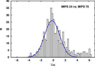
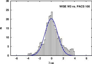
Figure 2.— Determining the calibration between MIPS 24 and 70 $\micron$, and WISE W3 and PACS 100 $\micron$. For displaying the data, the bins were smoothed using a three-bin running average.

3.3. PACS 100 $\micron$ data

The Herschel/PACS data were reduced using the Herschel Interactive Processing Environment (HIPE, V9.0 user release, Ott, 2010) and followed the recommended procedures. We generated the calibrated Level 1 product by applying the standard processing steps (flagging of bad pixels, flagging of saturated pixels, conversion of digital units to Volts, adding of pointing and time information, response calibration, flat fielding) and performed second-level deglitching with the “timeordered” option and a 20 sigma threshold (slightly more conservative than the recommended 30 sigma) to remove glitches. This technique uses sigma-clipping of the outlying flux values on each map pixel and is very effective for data with high coverage. After this stage the science frames were selected from the timeline by applying spacecraft-speed selection criteria (as recommended in the pipeline script, 18″/s $<$ speed $<$ 22 ″/s). The 1/f noise was removed using high-pass filtering with a filter width of 20 for the 100 $\mu$m data. This method is based on highpass median window subtraction; thus the images might suffer from loss of flux after applying the filter. To avoid this we used a mask with 20″  radius at the position of our sources. After high-pass filtering we combined the frames belonging to the two different scan directions and generated the final Level 2 maps using photproject also in HIPE. Aperture photometry was performed on the sources using a 12″  radius, while the sky background was determined with an aperture between 20″  and 30″. Six sub-sky apertures were placed within the nominal sky aperture with radii of 12″, to estimate the variations in the sky background. Each image was then inspected. In a few cases, interference by neighboring sources caused us to reject the photometry completely; in many more, there was a source in one of the six sub-sky apertures and the photometry was checked in place to circumvent the possible influence of this source on the results. Our self-calibration of the data to determine the photospheric level (detailed below) circumvents any residual calibration offsets. A summary of the photometry from the DUNES and the DEBRIS surveys as well as ages is presented in Table A.3.

There is a range of possible choices for the reduction parameters; ultimately, the validity of our reduction depends on testing it to see if: 1.) it provides accurate calibration; 2.) the noise is well-behaved; 3.) it can be validated against independent measurements; and 4.) it is free of systematic errors. We discuss each of these issues in turn.

In the case of the PACS 100 $\micron$ data, we determined the stellar photospheric ratio of WISE W4 22 $\micron$ flux density to that at 100 $\micron$ empirically, following the same routines as we performed for the MIPS 70 $\micron$ data calibration (Gordon et al., 2007). We judged the position of the peak in the $\chi_{100}$ distribution by Gaussian fitting and found it to be 3% above a simple Rayleigh-Jeans extrapolation. The far infrared spectral energy distributions of stars are not well understood observationally, but theoretical models indicate values of 1 - 2% above Rayleigh Jeans (Castelli, F.). For comparison, the absolute calibration at MIPS 24 $\micron$ has an uncertainty of 2% and that of PACS of 3 - 5%, so our reduction preserves the calibration to well within its uncertainties.

The uncertainties we derive are typical for PACS observations of similar integration time. However, a more stringent test is whether they are normally distributed. The distribution of $\chi_{100}$ is the distribution of differences from the photospheric flux density in units of the estimated standard deviation. As shown in Figure 2, it is acccurately Gaussian and falls to low levels at the 3-sigma point (the excess above 3-sigma toward the high end is due to debris-disk infrared excesses. Thus our reduction correctly estimates the noise and produces the expected noise distribution.

Examination of Table A.3 shows that the MIPS and PACS measurements are generally consistent, as we will demonstrate in more detail below when we discuss identifying the members of this sample with detected excess emission. A short summary is that, of 60 stars with the most convincing evidence for excesses, 56 were observed with both telescopes, and for 55 of these there is an indicated signal from each independently (¿ 3 sigma in one and at least 1.4 sigma with the other).

Finally, we have tested whether our measurements are subject to systematic errors due to missing some extended flux. We set the filtering and aperture photometry parameters at values to help capture the flux from extended debris disks. For the largest systems known, we still come up 20% (61 Vir - Wyatt et al., 2012) to 30% (HD 207129 - Löhne et al., 2012) short and we have substituted the values from the references mentioned for those we measured. However, for all 15 resolved systems in our sample and with studies in the literature (Booth et al., 2013; Broekhoven-Fiene et al., 2013; Matthews et al., 2010; Liseau et al., 2010; Eiroa et al., 2010; Kennedy et al., 2012), the average underestimate is 6.4%, and if we exclude 61 Vir and HD 207129 it is only 3.4%. This test is severe, since the literature will preferentially contain the most dramatic examples of extended disks; in fact, inspecting the DUNES/DEBRIS images there are only 2-3 clearly extended systems that are not yet the subject of publications (we note these in Table A.3). Nontheless, there appears to be little lost flux in our photometry.

3.4. Determining ages for the field sample stars

Ages were estimated for these stars using a variety of indicators. Chromospheric activity, X-ray luminosity, and gyrochronology as measures of stellar age are discussed by Mamajek & Hillenbrand (2008); we used their calibrations. To confirm the age estimates past 4 Gyr, we used a metallicity-corrected M_K vs. ${\rm V}-{\rm K}$ HR diagram and found excellent correspondence between the assigned ages and the isochrone age. This work is discussed in detail in J. Sierchio et al. (Submitted to ApJ). We also used values of $v\sin i>10~{}{\rm km}~{}{\rm s}^{-1}$ as indicators of youth, and $\log g<4$ as an indicator of post-main-sequence status (when other indications of youth were absent). Our assigned ages and the sources of data that support them are listed in Table A.3. We were not able to develop a rigid hierarchy among the methods in assigning ages, since occasionally an otherwise reliable indicator gives an answer that is clearly not reasonable for a given star – e.g., a low level of chromospheric activity can be indicated for a star whose position on the HR diagram is only compatible with a young age; HD 33564 is an example.

3.5. The decay of planetary debris disk excesses at 24 $\micron$

Spitzer 24 $\micron$ data have been used in many studies of warm debris disk emission (e.g., Rieke et al., 2005; Su et al., 2006; Siegler et al., 2007; Trilling et al., 2008; Gáspár et al., 2009). Given the uncertainties in the ages of field stars, stellar cluster studies, where numerous coeval systems can be observed, are strongly favored in disk evolution studies. The clusters included in our current research (Table 3) have well defined ages and, more importantly, homogenic and reliable photometry. Unfortunately, getting an even coverage of ages using only clusters is not possible, especially for ages above a Gyr, which is why we combined the stellar cluster studies with field star samples. We include the study of 24 $\micron$ excesses around early-type field stars by Su et al. (2006), while the solar-type stars are included from Sierchio et al. (Submitted to ApJ). We also include the Spitzer 24 $\micron$ measurements of the sources found in the DUNES and DEBRIS Herschel surveys (K. Y. L. Su, private communication). Our final combined samples have 721 and 376 sources in the solar-type (F5-K9) and early-type (A0-F5) groups, respectively. We summarize our detection statistics in Table 4.

Table 4The detection statistics of the observational sample. The columns give the detected number of debris disks over the total number of sources, as a function of age and observed wavelength, for each survey. The detection criteria are described in the text.

	Age	DUNES		DEBRIS		Additional†		Total
	(Myr)	24$\micron$	85$\micron^{\ddagger}$	24$\micron$	85$\micron^{\ddagger}$	24$\micron$	85$\micron^{\ddagger}$	24$\micron$	85$\micron^{\ddagger}$
Early(A0-F5)	1 - 31	0/0	0/0	1/3	1/3	64/130	-/-	65/133	1/3
	31 - 100	0/0	0/0	0/5	0/5	7/21	-/-	7/26	0/5
	100 - 316	0/1	0/1	10/18	10/18	14/57	-/-	24/76	10/19
	316 - 1000	0/0	0/0	7/54	8/54	9/67	-/-	16/121	8/54
	¿ 1000	1/3	2/3	1/17	4/17	-/-	-/-	2/20	6/20
Early Total		1/4	2/4	19/97	23/97	94/275	-/-	114/376	25/101
Solar(F5-K9)	1 - 31	0/1	0/1	0/2	0/2	58/125	2/6	58/128	2/9
	31 - 100	0/0	0/0	0/1	0/1	18/57	2/3	18/58	2/4
	100 - 316	1/3	3/3	0/5	0/5	34/98	8/27	35/106	11/35
	316 - 1000	1/16	6/16	0/30	1/30	5/86	8/39	6/132	15/85
	1000 - 3160	1/33	6/33	0/34	1/34	1/32	9/32	2/99	16/99
	¿ 3160	1/62	10/62	0/59	5/59	0/77	5/77	1/198	20/198
Solar Total		4/115	25/115	0/131	7/131	116/475	34/184	120/721	66/430
Total (A0-K9)		5/119	27/119	19/228	30/228	210/750	34/184	234/1097	91/531

For our current study, we are interested in the fraction of sources with excess as a function of stellar age. We defined a significant excess to occur when the excess ratio (defined as the ratio of the measured flux density to the flux density expected from the stellar photosphere) was $>1.1$ (see, e.g., Urban et al., 2012, for details of how this threshold is determined). Classically, sources are binned into age bins and then the fraction of sources with excess is determined for each age bin. Instead, we ran a Gaussian smoothing function over the observed age range, with a Gaussian smoothing width of 0.2 dex in $\log({\rm age})$. With this method, we generate smooth excess fraction (defined as the fraction of the sample of stars with excess ratios above some threshold, in this case above 1.1) decay curves. Errors of these decay curves were calculated using the method described in Gáspár et al. (2009). Our final smoothed decay curves at 24 $\micron$ with $\pm 1~{}\sigma$ errors for the early- and solar-type stars are shown in Figure 3. The solar-type stars show a slightly quicker decay between 0.1 and 1 Gyr, outside of the 1 $\sigma$ errors. We compare these decay curves with population synthesis models in Section 4.

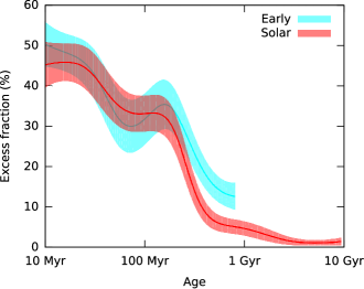
Figure 3.— The smoothed excess fraction decay curves at 24 $\micron$ for early- and solar-type stars, with 1 $\sigma$ error bars. The solar-type stars show a slightly quicker decay than the early-types.

3.6. The decay of planetary debris disk excesses at 70–100 $\micron$

The MIPS 70 and PACS 100 $\micron$ data are suitable for following the evolution of cold debris disks (Rieke et al., 2005; Su et al., 2006; Wyatt, 2008). The observations are inhomogenous, having non-uniform detection limits, which are frequently significantly above the stellar photospheric values. Due to this, unfortunately, a coherent disk fraction decay can not be calculated, such as for the 24 $\micron$ observations. We have developed new methods on analyzing the decay of the cold debris disk population, which we detail in Section 4.3.

We used the combined MIPS/PACS far infrared data to generate a reliable list of stars with far infrared excess emission. First, there are 35 stars with both $\chi_{70}$ and $\chi_{100}>4$ and 4 more measured only with PACS with $\chi_{100}>4$ (3 of them have $\chi_{100}>10$). Thirteen additional stars have $\chi$ measured with one telescope $\geq 4$ and $\chi$ with the other telescope $>2$. These 52 stars should constitute a very reliable ensemble of far infrared excesses. The remaining eight candidates are HD 7570 ($\chi_{70}=3.9$; $\chi_{100}=2.6$); HD 23281 ($\chi_{70}=8.6$ and $\chi_{100}=1.8$), HD 87696 ($\chi_{70}=3.0$ and $\chi_{100}=2.4$), HD 88955 ($\chi_{70}=4.0$ and $\chi_{100}=1.6$), HD 223352 ($\chi_{70}=6.0$ and $\chi_{100}=0.2$), HIP 72848 ($\chi_{70}=2.3$ and $\chi_{100}=3.2$). HIP 98959 ($\chi_{70}=3.7$ and $\chi_{100}=2.4$), and HIP 107350 ($\chi_{70}=4.5$ and $\chi_{100}=1.4$). In all these cases, there is a strong case for a detected excess with a promising indication of a far infrared excess with each telescope (excepting for HD 223352), so we add them to the list of probable excesses for a total of 60. Finally, HD 22001 has $\chi_{70}=0.85$, $\chi_{100}=8.3$; inspection of the measurements indicates that the probably far infrared spectrum does indeed rise steeply from 70 to 100 $\micron$. This behavior is expected of a background galaxy; in general the spectral energy distributions of debris disks fall (in frequency units) from 70 to 100 $\micron$. We therefore do not include this star in our list of those with probable debris disk excesses. Excluding this last star, the total combined DEBRIS/DUNES sample has 373 members. Of these, 347 are within our modeled spectral range (A0-K9) and have age estimates, of which 57 have probable debris disk excesses.

By comparing the results from both MIPS and PACS and also maintaining their independence, we have been able to identify reliably a set of stars with far infrared excess emission. We list the final photometric data for these sources in Table A.3. For our current study we also include the 70 $\micron$ measurements of Sierchio et al. (Submitted to ApJ). Our final catalog of far-IR measurements totals 557 sources, of which 531 are within our modeled spectral range (A0-K9) and have age estimates (101 early and 430 solar-type). However, we do not analyze the decay of far IR excess emission around early-type stars due to the intrinsic lack of data past 1 Gyr. The observational statistics on the far-IR sample can also be found in Table 4.

4. Population synthesis and comparison to observations

In this section, we compare the decay of infrared excesses predicted by our model, using population synthesis, to the observed fraction of sources with excesses at $24~{}\micron$ and to the distribution of excesses at 70 – 100 $\micron$. The two wavelength regimes are dealt with differently due to reasons explained in Section 3.

4.1. Disk locations

By fitting black body emission curves to IRS spectral energy distributions (SEDs), Morales et al. (2011) found that the majority of debris disks have just a cold component or separate cold and warm components. Mostly independent of stellar spectral type, the respective blackbody temperatures for the warm and cold components yielded similar values.

The warm component was found slightly above the ice evaporation temperature, with a characteristic blackbody temperature of 190 K. While the systems around solar-type stars have a narrower distribution in temperatures (99 to 200 K), the ones around A-type stars have a wider one (98 to 324 K). Assuming astronomical silicates as grain types in warm debris disks (where volatile elements are likely missing), we calculate the equilibrium temperatures of grains as a function of their sizes and radial distances around solar- and early-type stars. We show these temperature curves in the top panels of Figure 4. With green bands, we plot the particle size domain that is most effective at emitting at 24 $\micron$, when considering a realistic particle size distribution within the disks (Gáspár et al., 2012b). This is found by first solving

$$\frac{\partial F_{24\micron}(a)}{\partial a}\equiv 0\;,$$ (2)

and then assuming the range of particle sizes that are able to emit at or above 40% of the peak emission to be the effective particle size range. Since this calculation uses the modeled particle size distribution and realistic particle optical constants, it will differ from one system to the other. With gray bands, we show the relative number of systems found by Morales et al. (2011) at various system temperatures. According to these plots, the most common radial distance for warm debris disks (where the green band and gray bands intersect) is at $\approx 3-6$ AU around solar-type (G0) stars. This can be seen in the figure because the temperature curves for 3.5 and 5.5 AU pass through the intersection of the green and gray bands. A similar argument indicates a radial distance of $\sim 11$ AU for the early-type (A0) stars. However, a range of distances can be accommodated, especially if one considers grains with varying optical properties.

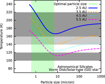
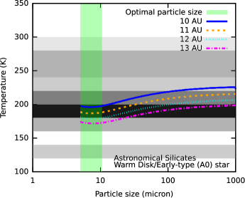
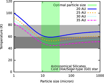
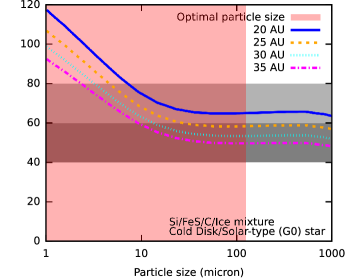
Figure 4.— Grain temperatures as a function of particle size, composition, radial distance, and the spectral type of the central star. The colored vertical bands yield the optimum particle size for emission (see text) around the certain systems, while the horizontal gray bands yield the relative number of systems (with 70 $\micron$ detections) found at each temperature (darker stand for more sources) by Morales et al. (2011). The plots yield the general radial distance of warm and cold debris disks around different spectral type systems where the colored bands, the gray bands, and the temperature curves intersect.

We performed similar analysis for the cold components, but only for the solar-type sample, as we do not have a statistically significant sample at old ages for the early-types. For the cold component analysis, however, we include a second grain-type, one that includes volatiles, as these disks are located outside of the snowline. We use the optical properties calculated by Min et al. (2011) for a Si/FeS/C/Ice mixture, which have been used to successfully model the far-IR emission and resolved images of Fomalhaut obtained with Herschel (Acke et al., 2012). We show these plots (green band - astronomical silicates; red band - volatile mixture), in the bottom panels of Figure 4. The plots estimate the cold disks to be located at around $20-35$ AU for an astronomical silicate composition and around $25-40$ AU for the volatile mixture. The latter estimate is more in agreement with the location of the Kuiper belt within our solar system. We can compare with disks around other stars by scaling their radii according to the thermal equilibrium distances, i.e., as $(L_{\ast})^{1/2}$. The locations for grains of the ice mixture generally agree with these scaled radii.

4.2. Modeling the 24 $\micron$ excess decay

Based on the previous section, to model the decay of the warm components, we calculated the evolution of debris disks at radial distances between 2.5 and 10 AU with 0.5 AU increments for solar-type stars (G0), and at radial distances between 9.0 and 14 AU with 1.0 AU increments for early-type stars (A0). The disk widths and heights were set to 10% of the disk radius, while the total disk mass was set to 100 $M_{\earth}$, assuming a largest object radius of 1000 km. All other parameters were the same as for our reference model (Paper II). In Figure 5, we show the evolution of the model debris disk at 4.5 AU around a solar-type star. The top left panel shows the evolution of the particle mass distribution in “mass/bin”-like units. The top right panel shows the evolution of the SED of the debris disk, with the color/line coding being the same as for the mass distributions. The SEDs were calculated assuming astronomical silicate optical properties (Draine & Lee, 1984). Both the mass distribution and the SED decay steadily in the even log-spaced time intervals we picked. The bottom left panel shows the evolution of the fractional 24 $\micron$ infrared emission, which (as with our reference model in Section 3) shows varying speed in evolution. The color/line codes show the points in time that are displayed in the top panels. The speed of evolution is shown in the bottom right panel. The evolution speed curve is very similar to that of the reference model in Section 2, however, the evolution is much quicker. While our reference model settles to the $\propto t^{-0.6}$ decay at around 100 Gyr, our warm disk model at 4.5 AU already reaches this state at 10 Myr. There are two reasons for this behavior: 1) The disk evolves quicker closer to the star (the reference model was at 25 AU), and 2) the extremely large initial disk mass (which was set to ensure coverage at large disk masses as well) significantly accelerates the evolution.

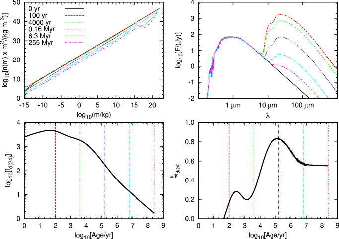
Figure 5.— Evolution of the warm disk component model around a solar-type star at 4.5 AU. Top-left panel: The evolution of the particle-mass distribution in “mass/bin”-like units. Top-right panel: Evolution of the SED of the disk (color coding is the same as for the top-left panel). Bottom-left panel: Evolution of the fractional 24 $\micron$ infrared emission as a function of age (the constant 5 Myr offset was applied later – see text). Bottom-right panel: The speed of the evolution of the fractional infrared emission. The evolution reaches its quickest point at 0.1 Myr, and settles to a $\propto t^{-0.6}$ evolution at around 10 Myr. The average mass disk in the population, which is barely detectable for a short period of time, would reach this at around 1000 Gyr; while a disk detectable between 0.1 – 1 Gyr reaches this quasi steady state around 1 Gyr.

To compare these models with observations, we will use the excess fraction (fraction of a population with excesses above a threshold) as the metric, since this is the parameter most readily determined observationally. We calculate the fraction of sources with excesses at a given age using the decay of a single source and using a population synthesis routine, by making two assumptions:

1. The distribution of initial disk masses follows a log–normal function.

2. All systems initiate their collisional cascade at the same point in time during their evolution. This point can not be earlier than the time of planet formation. We fix $t(0)$ at 5 Myr for our calculations.

Both assumptions are plausible. Our first assumption is consistent with observations of protoplanetary disks, as shown by Andrews & Williams (2005). In addition, this form was adopted by Wyatt et al. (2007) as the starting point for their analytic modeling of debris disk evolution, and thus adopting a similar initial form allows direct comparisons with this previous work. The log-normal form also gives a reasonably good fit to the distribution of excesses in young debris systems (J. Sierchio et al., Submitted to ApJ). We define the probability density distribution of the total disk masses as

$$n(M_{\rm tot};\mu,\sigma_{e})=\frac{1}{M_{\rm tot}\sqrt{2\pi\sigma_{e}^{2}}}{\rm Exp}\left\{-\frac{\left[\ln\left(M_{\rm tot}\right)-\mu\right]^{2}}{2\sigma_{e}^{2}}\right\}\;,$$ (3)

where $n(M_{\rm tot})$ is the probability density of systems with initial masses of $M_{\rm tot}$, the “location parameter” of the log–normal distribution is $\mu$, and $\sigma_{e}$ is the “scale parameter”. We set the scale parameter to be equal to the width of the distribution of protoplanetary disk masses found by Andrews & Williams (2005), $\sigma^{2}_{\rm e}=6.95\pm 0.06$ (in natural log base). Since the peak in the mass distribution depends on the largest mass within the systems and can be arbitrarily varied to a large extent, the location parameter is found by fitting. We set the median (geometric mean) of our log–normal distribution of masses to be equal to

$$CM_{\rm tot,0}={\rm e}^{\mu}$$ (4)

where $C$ is a scaling constant that yields the scaling offset between the median mass of the distribution and the mass of our reference model ($M_{\rm tot,0}=100M_{\earth}$).

The second assumption arises because the collisional cascades in debris disks cannot be maintained without larger planetary bodies shepherding and exciting the system. According to core accretion models, giant planets such as Jupiter and Saturn form in less than 10 Myr (Pollack et al., 1996; Ida & Lin, 2004), while disk instability models predict even shorter timescales (Boss, 1997, 2001). As planets form, simultaneously, the protoplanetary disks fade (Haisch et al., 2001), and their remnants transition into cascading disk structures. Based on these arguments, our $t(0)$ value of $5~{}{\rm Myr}$ is reasonable. Our assumption ignores the possibility of later-generation debris disks. That is, any late-phase dynamical activity that yields substantial amounts of debris will not be captured in our model, whose assumptions are similar to those of the Wyatt et al. (2007) analytic model in which the disk evolution is purely decay from the initial log-normal distribution.

A useful property of collisional models is that their evolution scales according to initial mass, which made the synthesis significantly simpler, as only a single model had to be calculated. The flux $f$ emitted by a model at time $t$ with an initial mass $M_{\rm tot}$ will be equal to a fiducial model’s flux $f_{0}$ with initial mass $M_{\rm tot,0}$ at time $t_{0}$ as

$$f(t)=f_{0}(t_{0})\frac{M_{\rm tot}}{M_{\rm tot,0}}$$ (5)

$$t=t_{0}\frac{M_{\rm tot,0}}{M_{\rm tot}}\;.$$ (6)

We verified that our model follows these scaling laws by running multiple models with varying initial disk masses (see Appendix). These relations are equivalent to a translation of the decay along a $t^{-1}$ slope, which is why as long as the decay of single sources remains slower than $t^{-1}$, the decay curves will not cross each other. Similar behavior has been shown by Löhne et al. (2008). This also means that each particular observed $f(t)$ value can be attributed to a particular initial disk mass and that at any given age the limiting mass can be calculated that yields a fractional infrared emission that is above our detection threshold.

To compare with the observationally determined percentage of sources above a given detection threshold, we need to find the initial mass whose theoretical decay curve yields an excess above this threshold as a function of system age. As detailed above, since the decay speed is always slower than $t^{-1}$, this will always be a single mass limit, without additional mass ranges. We can then calculate the cumulative distribution function (CDF) of the log–normal function using these initial mass limits [$M_{l}(t)$] defined as

$${\rm CDF}\left[M_{l}(t);\mu,\sigma_{e}\right]=\frac{1}{2}\left(1+{\rm erf}\left\{\frac{\ln\left[M_{l}(t)\right]-\mu}{\sqrt{2\sigma_{e}^{2}}}\right\}\right)\;.$$ (7)

Although the distributions get skewed in the number density vs. current mass (or fractional infrared emission) vs. age phase space, they remain log–normal in the number density vs. initial mass phase space, which is why this method can be used. The $\chi_{\rm fit}^{2}$ of our fitting procedure, where we only fit the location of the peak of the mass distribution, is then

$$\chi_{\rm fit}^{2}=\sum_{i}\frac{\left\{1-{\rm CDF}\left[M_{l}(t_{i});\mu,\sigma_{e}\right]-F\left(t_{i}\right)\right\}^{2}}{\sigma_{F}^{2}\left(t_{i}\right)}\;,$$ (8)

where $F\left(t_{i}\right)$ is the measured excess fraction at time $t_{i}$, and $\sigma_{F}^{2}\left(t_{i}\right)$ is the error of the measured excess fraction at time $t_{i}$. It is necessary to subtract the CDF from 1, because we are comparing the percentage of sources above our threshold and not below.

In Figure 6, we show the best fitting mass population and its evolution for the warm component of solar-type stars placed at 4.5 AU. The top panel shows the fractional infrared emission decay curves, shifted along the $t^{-1}$ slope as a function of varying initial disk masses. As the plot shows, the curves do not intersect, and they do not reach a common decay envelope (as is predicted by analytic models that yield a uniform $t^{-1}$ decay slope (e.g. Wyatt et al., 2007)). The decay curves do merge after 500 Myr of evolution, leaving a largely unpopulated (but not empty) area in the upper-right corner of the plot. Before 500 Myr, they occupy most of the phase space. For cold debris disks, the merging of the decay curves happens at an even later point in time. This also means that a maximum possible disk mass or fractional infrared emission at a given age, as predicted by the simple analytic models, does not exist; although with adjustments to the slower decay, after 500 Myr, they could approximate the evolution of the population. The color code of the plot shows the number of systems at any given point in the phase space. While systems show a spread in fractional infrared emission up to $\approx 100~{}{\rm Myr}$, after that they do increase in density along the decay curve of the average disk mass (shown with bold line) up to 10 Gyr, which is still faster ($\propto t^{-0.6}$ …$t^{-0.8}$) than the final quasi steady state decay speed of $\propto t^{-0.6}$. The bottom panel shows the evolution of the number distribution as a function of fractional 24 $\micron$ emission at different ages (vertical cuts along the top panel). The initial distribution at age 0 follows the initial mass distribution’s log–normal function; however, as the population evolves this gets significantly skewed. The black vertical line at $f_{d(24)}=0.1$ gives our detection threshold at $24~{}\micron$ and the lower integration limit for our excess fraction decay calculations.

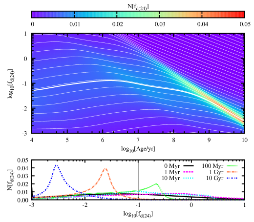
Figure 6.— The best fitting mass population and its evolution for the warm component of solar-type stars placed at 4.5 AU. Top panel: the fractional 24 $\micron$ emission decay curves ($f_{d(24)}=F_{\rm disk}(24)/F_{\ast}(24)$), shifted along the $t^{-1}$ slope as a function of varying initial disk masses. The color code of the plot is proportional the number of systems at any given point in the phase space. The bold line represents the evolution of the average mass disk in the population. Bottom panel: the evolution of the number distribution as a function of fractional 24 $\micron$ infrared emission at different ages (vertical cuts along the top panel). The initial fractional infrared emission distribution at age 0 follows the initial mass distribution’s log–normal function, however, as the population evolves this gets significantly skewed. The black vertical line at $f_{d(24)}=0.1$ gives our detection threshold at $24~{}\micron$ and the lower integration limit for our excess fraction decay calculations

Figure 7 shows the calculated $M_{l}(t)$ limit as a function of system age as well as the average mass of our modeled population ($\pm 1$ dex). The plot shows that any system with excess that is over a Gyr old could only be explained with the quasi steady state model if its initial mass was at least 3 - 4 orders of magnitude larger than the mass of our average disk. Since such massive disks are unlikely, these late phase excesses must arise from either a stochastic event or possibly from small grains leaking inward from activity in the outer cold ring.

Figure 7.— The mass of the disk at the detection limit as a function of system age [$M_{l}(t)$], and the evolution of the average disk mass ($\pm$ 1 dex) in the distribution.

In Figure 8, we show the excess fraction decay curves calculated from our best fitting population synthesis models at varying distances for the two different spectral groups. The left panel shows the models for the solar-type stars, while the right panel shows them for the early-type stars. The solar-types can be adequately fit with models at 4.5 and 5.5 AU, which matches reasonably well to the temperature peak observed by Morales et al. (2011). Similarly, we get adequate fits to the early-type population with models placed at 11 AU, which is also in agreement with the temperature peak observed by Morales et al. (2011) and our radial distance constraint.

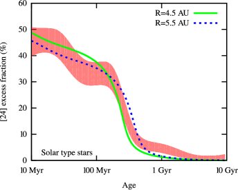
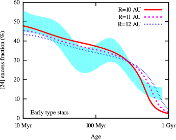
Figure 8.— The excess fraction decay curves calculated from our best fitting population synthesis models for warm disks at varying distances for the two different spectral groups. The right panel shows the models for the solar-type stars, while the left panel shows them for the early-type stars.

Our population synthesis routine yields excess fraction decays that are in agreement with the observations. This is the first time that a numerical collisional cascade code has been used together with a population synthesis routine to show agreement between the modeled and the observed decay of infrared excess emission originating from debris disks. The average initial disk mass predicted by our population synthesis has a total of 0.23 $M_{\rm Moon}$, with a largest body radius of $1000~{}{\rm km}$. This yields dust masses of $M_{\rm dust}(<1~{}{\rm cm})=2.3\times 10^{-5}~{}M_{\rm Moon}$ $=2.8\times 10^{-7}~{}M_{\earth}$ ($M_{\rm dust}(<1~{}{\rm mm})=7.3\times 10^{-6}~{}M_{\rm Moon}=9.0\times 10^{-8}~{}M_{\earth}$). Our predicted average dust mass is in agreement with the range of dust masses ($2.8\times 10^{-7}$ to $5.2\times 10^{-3}~{}M_{\rm Moon}$) observed by Plavchan et al. (2009) for debris disks around young low-mass stars, determined from infrared luminosities.

4.3. Modeling the far-IR (70–100 $\micron$) excess decay

According to section 4.1, to model the decay of the cold disks, we calculated the evolution of a disk placed at 15, 20, 25, 30, and 35 AU around a solar-type star. At these distances, volatiles are a large part of the composition, which will change not only the optical properties of the smallest grains (see section 4.1), but also the tensile strength of the material. To account for this, we used the tensile strength properties of water-ice from Benz & Asphaug (1999) and the erosive cratering properties of ice from Koschny & Grün (2001a, b). For comparison, we repeated the calculations with the tensile strengths of basalt, as in our reference model. The emission of the modeled particle size distributions was calculated assuming astronomical silicates for the regular basalt tensile strength models, and the volatile mixture (Min et al., 2011) mentioned in section 4.1 for the water-ice tensile strength models.

Understanding and modeling the decay observed at far-IR wavelengths is significantly more difficult than it is for its shorter, 24 $\micron$ wavelength, counterpart. This is due to the non-uniform detection limits at longer wavelengths, which are frequently significantly above the stellar photospheric values. Here, we will use the method developed by Sierchio et al. (Submitted tp ApJ) to study the evolution of the far-IR excess, but slightly modified to use our calculated evolved fractional infrared emission distributions. This new method quantifies the decay, taking into account both detections and non-detections and also the non-uniform detection limits.

We define the significance of an observed excess as

$$\chi=\frac{F-P}{\sigma}=\frac{R_{f}-1}{\sigma_{R}}\;,$$ (9)

where $F$ is the detected flux, $P$ is the predicted photospheric emission of the central star, while $\sigma$ is the error of the photometry. We define $R_{f}=F/P$ as the excess ratio of the source, and $\sigma_{R}$ as the photosphere normalized error.

The majority of the sources had both Spitzer 70 $\micron$ and Herschel PACS 100 $\micron$ data. We merged these data to simulate a single dummy 85 $\micron$ datapoint as

$$R_{f85}=\frac{R_{f70}/\sigma_{70}^{2}+R_{f100}/\sigma_{100}^{2}}{1/\sigma_{70}^{2}+1/\sigma_{100}^{2}}\;,$$ (10)

with an error of

$$\sigma_{R_{f85}}=\frac{1}{\left(1/\sigma_{70}^{2}+1/\sigma_{100}^{2}\right)^{1/2}}\;.$$ (11)

Since the excess ratios at 70 and 100 $\micron$ are similar, when measurement was only available at a single band, it was assigned to be at 85 $\micron$. As discussed in Sections 3.2 and 3.3, the definitions of excesses at the far-IR wavelengths are determined on a case-by-case basis for the detected disks. For the modeling comparison, a $\chi$ limit is required however, defining an excess. We chose $\chi_{85}>=3.7$ as our detection threshold, which recovers 63 of the 66 excess sources and adds only 2 false identifications.

We separate our observed sources into three age bins that cover the age range between 0 and 10 Gyr, the first bin including stars up to 1 Gyr (median age of sources: 475 Myr), the second including stars with ages between 1 and 4 Gyr (median age of sources: 2.65 Gyr), and the third with stars between 4 and 10 Gyr (median age of sources: 6.54 Gyr). These age bins were chosen to include equal numbers of sources (143,143, and 144, respectively).

We synthesize disk populations at 85 $\micron$ the same way as we did when modeling the $24~{}\micron$ excess decay, assuming a log–normal initial mass distribution, with the scale parameter fixed at $\sigma_{e}^{2}=6.95$, and varying only the location parameter of the distribution.

Finally, we compare the calculated distribution at 475 Myr, 2.65 Gyr, and at 6.54 Gyr, to the observed first, second, and third data bins, respectively. Since the detection thresholds are non-uniform, instead of doing a straight comparison between the distributions, we calculate the number of possible detections from our modeled distributions and compare with the observed distribution of excess significances ($\chi$’s). Assuming that the model distribution does show the underlying distribution of fractional far-IR excesses, we integrate the distribution upward from the detection threshold for each star in the corresponding data bin. The detection threshold is given as

$$\Theta=1+3\frac{\sigma}{P}=1+3\frac{R_{f}-1}{\chi}=1+3\sigma_{R}\;.$$ (12)

Integrating the distribution from the respective detection threshold of each source yields the probability of detecting an excess at the given threshold according to the model. Summing up these probabilities then yields the total number of predicted excesses that would be detected. This can then be compared to the actual number of observed excesses. The model that yields the best agreement for all three data bins consistently is defined as the best fitting model.

In Figure 9, we show the observed and modeled distribution of excesses at 30 AU, assuming water-ice tensile strength and the ice-mixture optical properties (the best fitting solution) in the three separate age bins. The observed sources are completeness corrected and sources below $R_{f}<1$ are not shown. For completeness correction, we assumed that the observed data well represents the photometric error distribution $\Gamma(\sigma_{R})$ of PACS observations. Then for each $\Delta R_{f}$ bin, we determined the probability of a source being in that bin, assuming the previously defined error distribution, yielding,

$$N_{s}(R_{f})=\int_{\sigma_{R-}}^{\sigma_{R+}}\Gamma(\sigma_{R})d\sigma_{R}\;,$$ (13)

where

$$\sigma_{R-} = \frac{R_{-}-1}{\chi_{\rm det}}$$ (14)

$$\sigma_{R+} = \frac{R_{+}-1}{\chi_{\rm det}}\;.$$ (15)

Here, $R_{-}$ and $R_{+}$ represent the lower and upper boundaries of the $\Delta R_{f}$ bin, respectively, as before $\sigma_{R}$ is the photospheric flux normalized error, and $\chi_{\rm det}$ is the detection threshold of $\chi$. We adopt $\chi_{\rm det}=3.7$ based on our data. The completeness correction than can be calculated as

$$C(R_{f})=\frac{N}{N-N_{s}(R_{f})}\;,$$ (16)

where $N$ is the total number of sources. In Figure 10, we show the completeness correction curve we derived for the combined DEBRIS and DUNES surveys at 100 $\micron$ for the three age groups we analyzed.

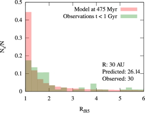
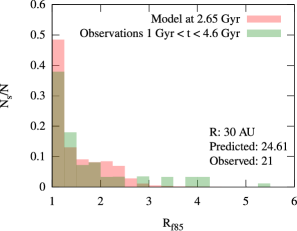
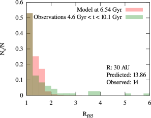
Figure 9.— The observed and modeled distribution of excesses at 30 AU around a solar-type star, using water-ice particle tensile strength and a volatile mix for grain optical properties. The best fitting model using the fiducial basalt tensile strength and astronomical silicates for grain properties yielded similar distributions, only at 17.5 AU radial distance.

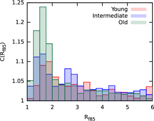
Figure 10.— The calculated completeness correction for the PACS 100 $\micron$ data. See text for details.

The panels in Figure 9 display the number of sources observed and predicted by our calculations in each given age bin. We emphasize, that the numbers of predicted sources are not determined based on these binned emission plots, but with the method detailed above. These plots show the emission distribution predicted by our fits and compare it with the completeness corrected observed distributions. The distributions are scaled to the total number of sources. The best fit for the basalt tensile strength and astronomical silicate optical property model (which looks almost identical to the ice mixture/strength solution plotted) was at $\approx 17.5~{}{\rm AU}$, which is clearly inwards of the predictions we made in section 4.1, and inwards of the cold disk component of our solar system. However, the water-ice composition and tensile strength model yields a fit at 30 AU, which is in agreement with the predictions and with the placement of the inner edge of the Kuiper belt in our solar system. In Table 5, we tabulate the number of predicted and observed sources for both models at various radial distances, and in Figure 11 we plot the relative differences between these numbers and show the predicted radial location of the disks with a red band. In Table 5, we also give the median masses of the best fitting distributions for each model. For our best fitting model (ice mixture particles at 30 AU), the median initial mass of the distribution is $0.028~{}M_{\earth}$, with a surface density of $1.3\times 10^{-3}~{}{\rm g~{}cm}^{-2}$, which is over four orders of magnitude times underdense compared to the minimum-mass-solar-nebula surface density.

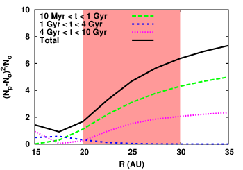
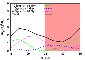
Figure 11.— The relative difference between the predicted and observed number of far-IR excess sources at solar-type stars, as a function of model radial distance. Left panel: Basalt tensile strength and astronomical silicate grain optical properties. Right panel: Water-ice tensile strength and volatile mixture grain optical properties.

Table 5The number of cold debris disk sources around solar-type stars predicted vs. the number of sources observed in each age bin at different disk radii , assuming varying optical properties and particle tensile strengths. The predicted radial location of the disks is between 20 to 35 AU for the silicate composition and 25 to 40 AU for the ice mixture. The median mass of the best fitting distribution is also given, assuming a largest body with a radius of 1000 km.

	$N_{P}/N_{O}$ for Silicates [$Q_{D}^{\ast}$(Basalt)]				$N_{P}/N_{O}$ for Si/FeS/C/Ice Mixture [$Q_{D}^{\ast}$(Ice)]
R	$M_{\rm med}$	0.01 …1	1 …4	4 …10	$M_{\rm med}$	0.01 …1	1 …4	4 …10
(AU)	($M_{\earth}$)	(Gyr)	(Gyr)	(Gyr)	($M_{\earth}$)	(Gyr)	(Gyr)	(Gyr)
15	0.051	29.61/30	24.21/21	10.37/14	0.397	36.00/30	18.78/21	11.74/14
20	0.029	24.19/30	23.57/21	15.88/14	0.092	34.93/30	20.48/21	8.98/14
25	0.023	20.35/30	21.92/21	18.63/14	0.039	29.28/30	24.61/21	10.05/14
30	0.024	18.64/30	21.18/21	19.38/14	0.028	26.14/30	24.61/21	13.86/14
35	0.026	17.76/30	20.85/21	19.72/14	0.022	22.50/30	23.29/21	17.16/14

4.4. Disk incidence for old stars

At 24 $\micron$, our model suggests there should be virtually no detected debris disks around stars older than 1 Gyr. Nonetheless, there are a number of examples, and examination of their ages indicates that they are of high weight. This result implies that the simple assumption (e.g., Wyatt et al., 2007) that debris disks can be modeled consistently starting from a log-normal initial mass distribution is successful up to about a Gyr, but that there are additional systems around older stars above the predictions of the simple model. We attribute these systems in part to late-phase dynamical activity that has led to substantial enhancements in dust production. Two examples in our sample are HD 69830 (Beichman et al., 2005) and $\eta$ Crv (Lisse et al., 2012). Another example is BD+20 307 (Song et al., 2005). All three of these systems have strong features in their infrared spectra that indicate the emission is dominated by small grains that must be recently produced, which supports the hypothesis that they are the sites of recent major collisional events. These systems with late phase 24 $\micron$ excess, however, could also be explained by grains leaking inward from an active cold ring.

Similarly, although our model successfully matches the numbers of detected disks in the far infrared, the observations find many more large excesses than predicted (Figure 9, bottom panel). A plausible explanation would be that the outer, cold disk component can also have renaissance of dust production due to late phase dynamical activity.

5. Constraining model parameters with observations

We ran more than a hundred extra models, taking our best fit to the decay of the warm component of solar-type debris disks at 4.5 AU as the basis, to test the dependence of the decay on the variables of the model. We varied each model parameter within a range of values and performed the same population synthesis routine and fitting as we did in Section 4. Of these, nine variables show signs of having some effect on the evolution of the excess fraction decay curve. In Figure 12, we present the reduced $\chi^{2}$ minima at each value of these nine parameters.

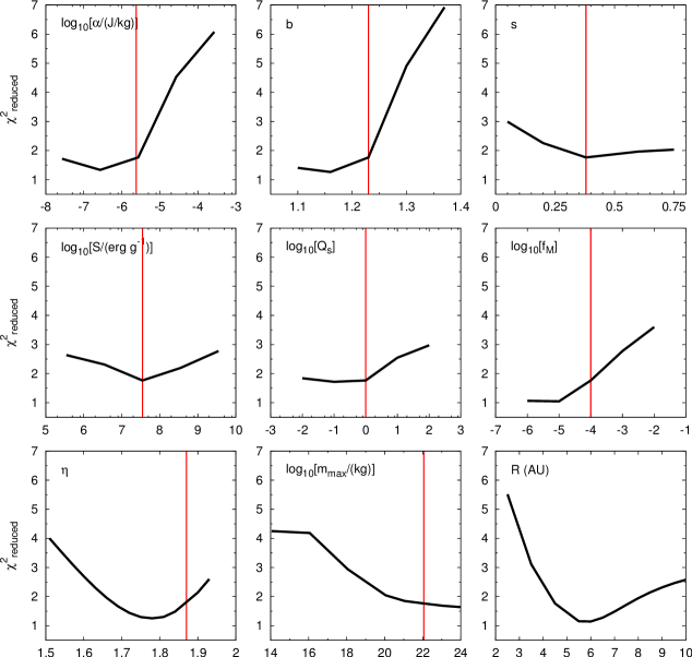
Figure 12.— The reduced $\chi^{2}$ minima of the model population fits for each tested value of the selected nine model variables that have the largest effects within the fits. Red lines show the values of variables used in the base model (the warm debris disk around a solar-type star at 4.5 AU introduced in Section 4.2).

Variables $\alpha$ and $b$ of the cratered mass equation had the strongest effect on the slope of the evolution (see Appendix) and also strongly affect the population synthesis fits. Values of $\alpha$ and $b$ that describe materials that are softer in erosive collisions ($\alpha>10^{-5}$ J kg^-1, $b>1.27$) can be generally ruled out by our analysis for the warm component of debris disks. Our analysis also shows that the measured values of these variables, which we used in our reference models, yield acceptable fits with our population synthesis routine. This is similar to the effect we observed when using water-ice erosive properties for the cold disk components in the previous section.

While the value of the slope of the tensile strength curve $s$ significantly affects the slope of the particle mass-distribution (O’Brien & Greenberg, 2003; Gáspár et al., 2012b), it does not affect the decay of the fractional infrared emission to the level where we would observe offsets between the modeled and observed rates. However, we do have a best fit at its nominal value.

The effects of varying $S$ and $Q_{s}$ are roughly the same as when varying $s$. As it turns out, the exact value of the tensile strength law does not strongly influence the decay of the excess fractions in a population of debris disks. However, choosing a higher value for $f_{M}$, which gives the interpolation distance between the erosive and catastrophic collisional domains, does result in less acceptable fits. This is an arbitrarily chosen numerical constant, and this analysis shows that choosing its value wisely is important. Based on these findings, we conclude that for our cold disk models in the previous section, the changes to $\alpha$ and $b$ when assuming a water-ice strength for the erosive collisions had a larger effect on the evolution than the changes to the catastrophic collision properties of the tensile strength curve.

While varying $\eta$ (the initial particle mass distribution slope) of a single disk will have significant effects on the timescale of its evolution (see Appendix), it does not strongly determine the timescale of the excess fraction evolution of a population. To compensate for the offset in timescales, the average disk mass varies from population to population (within an order of magnitude). Testing the actual value of the initial particle mass distribution is possible, by comparing the disk mass distributions predicted for each population to observations (such as in young clusters).

Varying the maximum mass $m_{\rm max}$ of the system did not have a large effect on the population synthesis fits above $10^{18}~{}{\rm kg}$, which reinforces our previous statement that it is the dust density of the model that matters and not an absolute total mass or largest mass in the system, which are redundant variables. However, very low maximum mass systems ($<10^{18}~{}{\rm kg}$ – $\approx 100~{}{\rm km}$ diameter) will result in decays that are inconsistent with our observations. This also has the important consequence, that the evolution of the planetary systems has to reach the point where bodies on this size scale are common in order to have a “successful” collisional cascade.

The radial distance of the model ($R$) obviously is the dominant parameter. In section 4.2, we showed that the best fit of our model to the observations is at $R\approx 4.5-5.5~{}{\rm AU}$, which agrees with the thermal location predicted by Morales et al. (2011). Here, we show the quality of the fits when varying the radial distance between 2.5 and 10 AU. Placing the disks closer than 4 or further than 8 AU yields a population decay that is inconsistent with the observations. This value can likely be modified to some extent by varying some of the other input variables of the model.

6. Conclusions

In this paper, we present a theoretical study of the evolution of debris disks, following their total disk mass ($M_{\rm tot}$), dust mass ($M_{\rm dust}$), and fractional 24 $\micron$ infrared emission ($f_{d(24)}$). We use the numerical code presented in Paper I that models the cascade of particle fragmentation in collision dominated debris disk rings.

Observational studies in the past decades have shown that the occurrence and strength of debris disk signatures fade with stellar age (e.g., Spangler et al., 2001; Rieke et al., 2005; Trilling et al., 2008; Carpenter et al., 2009). Analytic models of these decays explained them as a result of a steady-state (equilibrated) collisional cascade between the fragments (e.g., Spangler et al., 2001; Dominik & Decin, 2003; Wyatt et al., 2007), which results in a decay timescale proportional to $\propto t^{-1}$ for all model variables ($M_{\rm tot}$, $M_{\rm dust}$, $f_{d(24)}$). Analysis of the observed decays of stellar populations, however, has shown that the dust mass and the fractional infrared emission – the observable parameters – decay less quickly (Greaves & Wyatt, 2003; Liu et al., 2004; Moór et al., 2011, e.g.,). Slower decays have also been modeled by complete numerical cascade models (e.g., Thébault et al., 2003; Löhne et al., 2008; Kenyon & Bromley, 2008). Numerical codes yield slower decays because they model the systems as relaxing in a quasi steady state, instead of in complete equilibrium. This means that mass is not entered at the high mass end into the system (like in an analytic model), but is rather conserved. The remaining discrepancies among the numerical models are results of the different collisional physics and processes modeled within them.

Our calculations show that the evolution speed constantly varies over time and cannot be described by a single value. Since the fractional infrared emission is a proxy for the dust mass, their decays closely follow each other. At its fastest point in evolution, the total mass of our models decays as $M_{\rm tot}\propto t^{-0.33}$, while the dust mass and fractional infrared emission of the single disk decays $\propto t^{-0.8}$. At later stages in evolution these slow down to $\propto t^{-0.08}$ and $\propto t^{-0.6}$, respectively. These results are mostly in agreement with the models of Kenyon & Bromley (2008). We roughly agree with the dust mass decay predicted by the Wyatt et al. (2011) models up to the point where Poynting-Robertson drag (PRD) becomes dominant in their models (although their models decay somewhat faster than ours, possibly due to the constant effects of PRD).

We perform a population synthesis routine, assuming a log–normal probability distribution of initial disk masses. We calculate excess fraction decay curves, which we fit to the observed fraction of warm debris disks at a 10% excess threshold at 24 $\micron$. Our fits show a good agreement between the calculated and observed decay rate of the fraction of debris disk sources around both solar and early-type stars, with initial mass ranges in agreement with the distribution of protoplanetary disk masses (Andrews & Williams, 2005). We also analyze data from the MIPS/Spitzer and the DEBRIS and DUNES Herschel Space Observatory surveys. Taking into account the non–uniform detection thresholds at these longer wavelengths, we also show good agreement between the number of sources predicted to have an excess from our population synthesis routines and that observed within these surveys. The best correspondence between models and observations requires grains that are relatively weak and have optical constants similar to those of water-ice composites. However, a full range of grain properties was not explored.

There are a small number of bright debris disks at 24 $\micron$ around old stars that are not predicted by the simple decay from a log-normal starting distribution; they [HD 109085, HIP 7978 (HD 10647), HIP28103 (HD 40136), HIP40693 (HD 69830), $\eta$ Crv (HD 109085)] probably in part represent late-phase dynamical activity. Similarly, the model fails to fit the large excesses in the far infrared around old stars, again consistent with late-phase activity around a small number of stars.

Appendix A The system variables and their effects on the evolution of the collisional cascade

As we have shown in Section 5, varying the parameters of the model can affect the results of the population synthesis. Here, we analyze the effects of varying them on a single system. We summarize and describe the variables of the model in Table 6.

Table 6Numerical, Collisional, and System parameters of our model and their fiducial values

Variable	Description	Fiducial value
System variables
$\rho$	Bulk density of particles	2.7 g cm-3
$m_{\rm min}$	Mass of the smallest particles in the system	1.42$\times 10^{-21}$ kg
$m_{\rm max}$	Mass of the largest particles in the system	1.13$\times 10^{22}$ kg
$M_{\rm tot}$	Total mass within the debris ring	1 $M_{\earth}$
$\eta_{0}$	Initial power-law distribution of particle masses	1.87
$R$	Distance of the debris ring from the star	25 AU
$\Delta R$	Width of the debris ring	2.5 AU
$h$	Height of the debris ring -	2.5 AU
Sp	Spectral-type of the star	A0
Collisional variables
$\gamma$	Redistribution power-law	11/6
$\beta_{X}$	Power exponent in X particle equation	1.24
$\alpha$	Scaling constant in $M_{\rm cr}$	$2.7\times 10^{-6}$
$b$	Power-law exponent in $M_{\rm cr}$ equation	1.23
$f_{M}$	Interpolation boundary for erosive collisions	$10^{-4}$
$f_{Y}$	Fraction of $Y/M_{\rm cr}$	0.2
$f_{X}^{\rm max}$	Largest fraction of $Y/X$ at super catastrophic collision boundary	0.5
$Q_{\rm sc}$	Total scaling of the $Q^{\ast}$ strength curve	1
$S$	Scaling of the strength regime of the $Q^{\ast}$ strength curve	$3.5\times 10^{7}$ erg/g
$G$	Scaling of the gravity regime of the $Q^{\ast}$ strength curve	0.3 erg cm3/g2
$s$	Power exponent of the strength regime of the $Q^{\ast}$ strength curve	-0.38
$g$	Power exponent of the gravity regime of the $Q^{\ast}$ strength curve	1.36
Numerical parameters
$\delta$	Neighboring grid point mass ratio -	1.104
$\Theta$	Constant in smoothing weight for large-mass collisional probability	$10^{6}m_{\rm max}$
$P$	Exponent in smoothing weight for large-mass collisional probability	16

A.1. Evolution of the system mass

We show the total mass decay curves as a function of model variables in Figure 13 and the evolution of the power exponent of time in the decay of the total mass [$M_{\rm tot}(t)\propto t^{-\xi}$] as a function of these collisional variables in Figure 14. The figures include plots for the twelve variables that have the largest effect on the evolution, out of the total twenty-four variables (see Paper I). These decays are compared to that of our reference model, detailed in section 2.1.

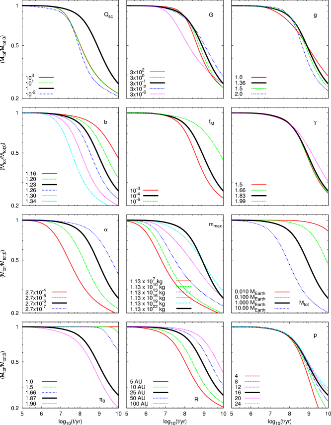
Figure 13.— Evolution of the total disk mass as a function of selected parameters that have the largest effect on the timescale of the evolution. The numerical variable $p$ modifies the smoothing function of the collisional cross section of the largest bodies in the system. The smoothing function only varies the evolution of the total mass (shown here), but does not affect the evolution of the dust mass or the fractional infrared emission.

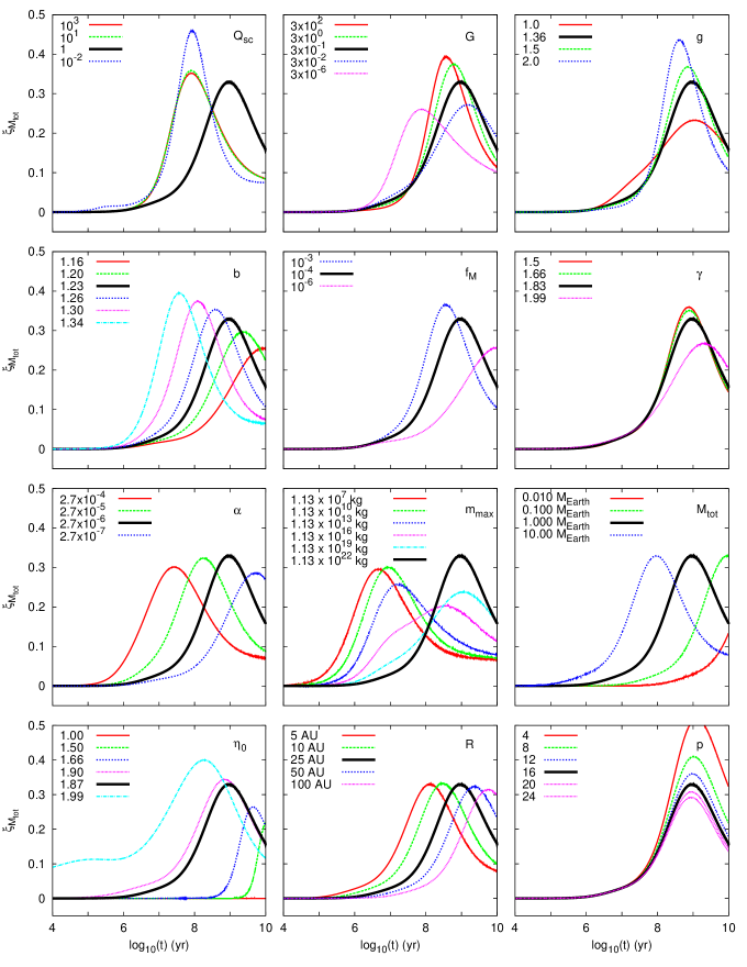
Figure 14.— The evolution of the power exponent of time in the decay of the total system mass [$M_{\rm tot}(t)\propto t^{-\xi}$] as a function model variables for decay curves shown in Figure 13. At its fastest point, our reference model decays with $\xi=0.33$, while all models reach a fastest point between $0.3<\xi<0.4$. The evolution of the power exponent is characteristic for all models, with an acceleration in evolution up to a certain point, from whereon the evolution of the total mass slows down.

In our code, we use the models of Benz & Asphaug (1999) to estimate the collision tensile strengths of particles, written as

$$Q^{\ast}(a)=10^{-4}\frac{\rm J~{}g}{\rm erg~{}kg}Q_{\rm sc}\left[S\left(\frac{a}{1~{}{\rm cm}}\right)^{s}+G\rho\left(\frac{a}{1~{}{\rm cm}}\right)^{g}\right]\;,$$ (A1)

where $a$ is the target particle’s radius, $Q_{\rm sc}$ is the total scaling of the curve, $S$ is the scaling of the curve in the “strength dominated” regime, $s$ is the power exponent of the target radii in the “strength dominated” regime, $G$ is the scaling of the curve in the “gravity dominated” regime, $\rho$ is the bulk density of the particles, and $g$ is the power exponent of the target radii in the “gravity dominated” regime. Of these, we show the effects of varying $Q_{\rm sc}$, $G$, and $g$, as varying $S$ and $s$ will not have a significant effect on the decay of the total mass, because they influence the low mass end of the distribution. Increasing or decreasing the total scaling will speed up the evolution of the total mass. Decreasing the total scaling of the tensile strength curve will soften the materials, resulting in a faster decay. Increasing it, however, will strengthen the materials, which will make the largest bodies “indestructible”, resulting in a faster decay in the number of bodies just below the high mass end. A similar effect can be seen when $G$ is varied.

The total mass cratered in an erosive collision is calculated in our model by applying the experimental results of Koschny & Grün (2001a, b). This mass is a function of $\alpha$ (scaling constant) and the projectile’s energy to the $b$ power. Variations in these constants will affect how quickly the largest bodies erode and subsequently, the evolution of the total disk mass. When softer material properties are used ($\alpha$ and $b$ increase), the decay is quicker, for example meaning debris disks composed of ice are likely to disappear in a shorter timescale than rocky debris disks.

The Koschny & Grün (2001b) formula for cratered mass in an erosive collision is only valid for relatively small cratered masses. The cratered mass given by the formula can exceed $M/2$ even below the Erosive/Catastrophic collision boundary. We thus interpolate the cratered mass from $f_{M}=M_{\rm cr}/M$ to the boundary via methods given in Paper I. Assigning it a very small value basically eliminates the erosive formula of Koschny & Grün (2001b) and uses an interpolative formula for the entire domain. However, a larger value is likely to overestimate the cratered mass in an erosive collision near the erosive/catastrophic collision boundary. Our approach was to use a conservative value within these extremes.

The number densities of fragments created in collisions in our model follow a power-law distribution. The slope of this distribution is given by $\gamma$, and only very minor effects can be seen when varying its value. The actual redistribution function has been a long researched topic within collisional systems, with some research showing that double or even triple power-law functions are the best to describe the fragment distributions (Davis & Ryan, 1990). According to our models, as long as the distribution function is within reasonable limits ($\gamma<1.99$ - mass is concentrated in the largest fragments), there is not much difference in the decay of the total mass when varying its value.

The total mass within the disk, $M_{\rm tot}$, sets the scaling of the particle size distribution (as do $m_{\rm max}$ and the volume of the disk). When scaling the initial total mass in the system, with all other parameters fixed, the evolution of the total mass is shifted in time, with the systems reaching their points of fastest decay at later points in time. This property is used in our population synthesis calculations in section 4.

The decay is dependent on the mass of the largest body $m_{\rm max}$, which is usually arbitrarily chosen in the numerical models. This shows in our calculations in Section 5, where going below a largest body mass of $10^{18}~{}{\rm kg}$ ($\approx 100~{}{\rm km}$ diameter) will result in decays that are inconsistent with our observations. When testing this for a single system, we set the total mass of the system to a value that yielded the same scaling of particle densities as the fiducial model had. This way we guaranteed that our calculations were only testing how varying the cutoff of the mass distribution affects the evolution.

The slope of the initial distribution, $\eta$, determines the number of dust particles when the collisional cascade is initiated. Our convergence tests (Paper I) have shown that the systems will reach collisional equilibrium from all initial distribution slope values. However, the time when the system reaches equilibrium will depend on the value of $\eta$. A system will be able to reach equilibrium from slope values lower than the steady-state cascade distribution faster than from steeper slopes, as it is easier to produce and build up dust sizes, than to remove the large massive particles from the highest masses.

One of the most important system variables is $R$, the distance of the disk from the central star. This parameter has many effects, as it sets the collisional velocity, thus the collisional energy of the particles and their collisional rate. It will also set the removal timescale for the blowout particles and is a variable in the volume of the disk, thus it sets the number density of the particles in the disk as well. Increasing the the radial distance will decrease the evolution rate of the disks, as shown in our Figures 13 and 14, with the fastest evolution setting in at later points in time.

The last parameter we analyze is $p$, which is a variable that sets the smoothing function of the collisional rates for the largest bodies in the system (Paper I). Its value only affects the evolution of the largest masses, thus also the evolution of the total mass in the system.

A.2. Evolution of the dust mass and fractional infrared emission

As we have shown before, the fractional infrared emission is a proxy of the dust mass in the system, meaning the decay curves and the analysis we give for the fractional infrared emission are generally identical to the one we would give for the dust mass in the system. For said reasons, we omit the plots for the evolution of the dust mass.

The emission of the particles depends on their temperatures, their sizes, and material and wavelength dependent optical properties, such as their absorption coefficients. We assume a Castelli & Kurucz (2003) intensity emission model for the stars and astronomical silicate optical constants for the particles (Draine & Lee, 1984), when calculating their equilibrium temperatures and emission.

We analyze the same parameters as in the previous subsection, with the exception of $G$, $g$, and $p$, which are replaced by $S$, $s$, and $\delta$. In Figure 15, we show the decay of the fractional infrared emission as a function of the model variables that have the largest effect on it, while in Figure 16, we show the power exponent of time in the decay. These figures can be compared the the evolution of the infrared emissions of our reference model, which is plotted with a thick solid line in the Figures and also analyzed in section 2.3.

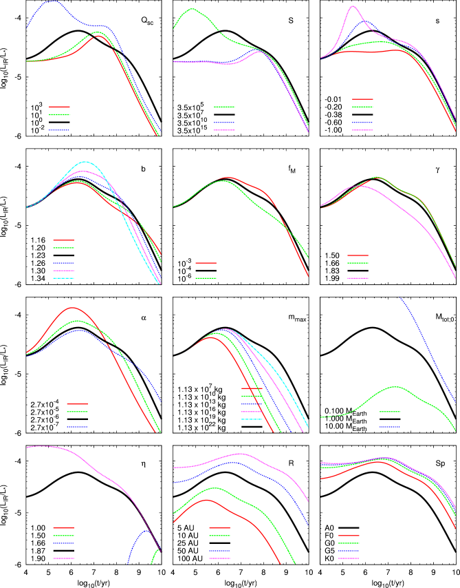
Figure 15.— Evolution of the fractional infrared luminosity as a function of selected parameters that have the largest effect on the timescale of its evolution. The characteristic bump seen in the evolution of the dust mass is reflected in the evolution of the infrared emission as well. The bump is followed by a drop in emission, which follows the same power-law as the drop in dust mass. Systems generally reach the quasi steady state decay at $\sim 100~{}{\rm Myr}$, although variations in this are seen as a function of model parameters.

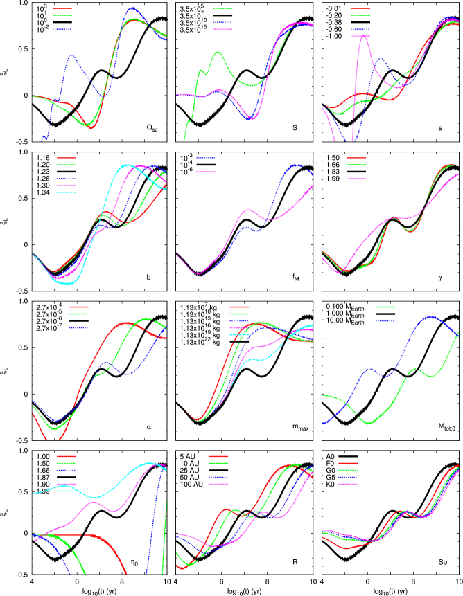
Figure 16.— The evolution of the power exponent of time in the decay of the fractional infrared luminosity as a function model variables for decay curves shown in Figure 15. At its fastest point, the infrared emission our reference model decays with $\xi=0.8$, while all models reach a fastest point between $0.6<\xi<0.9$. These model results generally agree with observations of disk decay.

The variables of the tensile strength curve that determine the strengths of the gravity dominated larger bodies ($G$, $g$) do not affect the evolution of the dust distribution, while the variables that determine the tensile strengths of the smaller particles ($S$, $s$) do. Increasing or decreasing the scaling of the tensile strength law ($Q_{\rm sc}$) increases the evolution speed for the dust mass, and thus the fractional infrared emission. At increased material strengths the quick decay of the largest bodies affects the evolution of the dust mass, while for softer materials a general faster decay of the entire distribution can be seen (see Figure 4 in Paper II). However, only significant decreases in the strength scaling $S$ will have noticeable effects in the evolution of the fractional infrared emission. Increasing the steepness of the tensile strength law $s$ will shift the evolution in time. Of all collisional variables, arguably $b$ and $\alpha$ are the most important. As expected, using softer erosive material properties (larger $b$ and $\alpha$) speeds up the evolution of the dust mass (and with that the evolution of the fractional infrared emission).

Changes in $f_{M}$ and $\gamma$ affect the evolution of the fractional infrared emission similarly to that of the total mass. Increasing the largest body in the system ($m_{\rm max}$) slows down the evolution of the collisional cascade, with models reaching their peak dust mass evolution at later stages, while increasing the total mass $M_{\rm tot}$ in the system will speed the evolution of the system, with higher total mass systems reaching their peak evolutionary point earlier on. Systems initiating their collisional cascades with varying initial mass-distribution slopes ($\eta_{0}$) will reach their quasi steady state dust mass decay (the peak of evolution speed) roughly at the same time, even though the beginning of the evolution is dependent on the slope. Debris rings located at different radial distances ($R$) will evolve with speeds associated with their orbital velocities, shifting the onset of their quasi steady state decay to later points in time for disks at larger radial distances.

Since $p$ is the smoothing function of the largest bodies, it also does not affect the evolution of the dust mass; however, the neighboring grid point mass ratio ($\delta$) will be numerically important. In Figure 15, we show that our models converge in dust mass decay at around 400-800 grid points, while using a less dense grid will result in numerical errors.

A.3. Conclusion

Our analysis above has revealed that erosive collisions are dominant in shaping the evolution of a debris disk. The evolution speed of our model is determined primarily by the variables ($\alpha$ and $b$) of the cratered mass equation, when considering fixed system variables. This is not that surprising, considering that $b$ also was found to be dominant in determining the mass-distribution slope (Paper II), and that our population synthesis analysis in section 5 also revealed that our fits are sensitive to the values of $\alpha$ and $b$. The evolution is much less dependent on the catastrophic tensile strength than on the erosive, which is surprising, considering the dependence of the particle mass-distribution slope on $s$ (O’Brien & Greenberg, 2003, Paper II).

The measurements of Koschny & Grün (2001a, b) give the value of $\alpha$ for silicates as $2.7\times 10^{-6}~{}{\rm kg~{}J}^{-1}$, and $6.2\times 10^{-5}~{}{\rm kg~{}J}^{-1}$ for ice; and a value of 1.23 for $b$. Measurements by Hiraoka et al. (2008) yield a $b$ value of 1.15, which is in agreement with the value given by Koschny & Grün (2001a, b) and yields an even better fit for our population synthesis constraint in section 5 ($\alpha$ values cannot be compared as the papers used slightly different equations).

Of the system variables, the evolution will most strongly depend on $\eta_{0}$, $R$, and $m_{\rm max}$. The evolution converges above $m_{\rm max}=1\times 10^{19}~{}{\rm kg}$ ($\approx 200~{}{\rm km}$ diameter), which most systems likely achieve (considering the asteroid sizes in our Main Asteroid Belt), making this variable less important for realistic conditions. Although $\eta_{0}$ is difficult to constrain, it is likely that the system will form with a mass-distribution slope with a value close to its quasi steady state solution. However, even if a system does not, its evolution still can adequately reproduce our observations according to our population synthesis calculations in section 5.

The radial distance of the disk is the overall dominant parameter in determining the evolution of a single disk, when all realistic conditions are considered. It influences the evolution by three independent effects, all acting in the same direction. At larger radii, the collisional velocity will be lower (thus the collisional energy will be lower), which lowers the effective mass range a particle can interact with. The reduced collisional velocity also reduces the collisional rate. Finally, an increase in radial distance increases the effective volume the disk encompasses (for the same amount of mass and disk aspect ratio), also resulting in reduced collisional rates.

Table 2Photometry of the DEBRIS and DUNES surveys.

						MIPS						PACS			Far
Name	Sp.	Age	P24	P70	P100	$F_{\rm 24}$	$\sigma_{\rm 24}^{\ast\ast}$	$R_{\rm 24}^{\Box}$	$F_{\rm 70}$	$\sigma_{\rm 70}$	$\chi_{\rm 70}$	$F_{\rm 100}$	$\sigma_{\rm 100}^{\ddagger}$	$\chi_{\rm 100}$	IR	Age◇	Age ref.
	type	(Gyr)	(mJy)	(mJy)	(mJy)	(mJy)	(mJy)	(mJy)	(mJy)	(mJy)		(mJy)	(mJy)		Exc?	Flagstring
DEBRIS survey (HD sources only)
HD000038	K6V	1.15	60	6.63	3.33	-	-	1.00	-	-	-	11.14string	4.96	1.56	N	2	1;2
HD000739	F5V	2.15	161	18.01	8.71	163	1.63	1.01	20.11	2.59	0.76	21.19string	7.87	1.57	N	1	3
HD001237	G8V	0.30	84	9.28	4.59	84	0.85	1.01	11.81	2.00	1.21	-4.26string	3.38	-2.61	N	3	2;3;4;5;6
HD001326	-	-	236	26.08	12.42	-	-	-	-	-	-	17.45string	5.11	0.97	N	-	-
HD001404	A2V	0.45	129	14.27	7.06	155	1.56	1.20	43.82	6.12	4.55	27.78string	2.68	6.86	Y	2	7
HD001581	F9.5V	3.82	557	61.55	29.23	557	5.57	1.00	71.20	5.73	1.43	45.25string	4.63	3.11	N	3	3;5;6;8
HD001835	G3V	0.44	80	8.84	4.37	-	-	1.06	-	-		22.41string	6.42	2.77	N	3	2;3;5;6;9;10;11;12;13;14
HD002262	A5IVn	0.72	282	31.14	15.02	310	3.10	1.10	72.97	2.52	9.43	34.45string	4.50	4.03	Y	2	7
HD003196	F7V+G4V	0.36	213	24.42	11.43	221	2.22	1.04	21.17	6.02	-0.53	19.40string	4.95	1.58	N	3	2;4;15;16
HD004391	G3V	1.20	136	15.03	7.63	-	-	1.01	-	-	-	18.90string	7.25	1.54	N	3	2;3;4;5;6
HD004628	K2.5V	5.20	276	31.38	14.67	284	2.85	1.03	-	-	-	24.69string	4.42	2.18	N	3	2;3;4;5;6;12;13;14;15
HD004676	F8V	5.30	209	23.54	11.51	213	2.13	1.02	30.33	5.89	1.12	18.67string	6.20	1.14	N	2	2;15
HD004747	G9V	2.25	55	6.08	2.92	55	0.56	1.00	2.08	3.41	-1.17	10.02string	2.77	2.52	N	3	2;3;9;10;12
HD004967	K7Vk	1.34	38	4.20	2.11	-	-	0.98	-	-	-	2.25string	6.39	0.02	N	1	3
HD005448	A5V	0.60	275	30.39	15.40	-	-	1.01	-	-	-	23.12string	7.91	0.97	N	2	7
HD007439∗	F5V	2.20	175	20.22	9.63	183	1.84	1.05	13.97	7.12	-0.87	12.05string	5.82	0.41	N	2	2;15
HD007570	F9VFe	5.30	249	28.62	13.01	259	2.59	1.04	46.54	3.94	3.92	30.45string	6.65	2.56	Y	3	2;3;5;17
HD007788	F6V+K1V	0.70	244	26.96	14.03	-	-	0.97	-	-	-	27.24string	5.25	2.44	N	3	2;16;18
HD009540	K0V	1.50	62	6.63	3.29	60	0.61	0.98	-2.26	4.90	-1.81	-2.36string	3.29	-1.72	N	3	2;3;4;9;10;11;12
HD010307	G1.5V	6.95	279	32.38	15.33	293	2.94	1.05	38.86	5.48	1.12	19.49string	4.98	0.82	N	2	6;15
HD010361†	K5V	4.57	472	52.15	26.48	-	-	1.01	-	-	-	23.09string	4.03	-0.81	N	3	3;5;6;14
HD010476	K1V	4.99	385	40.00	18.86	362	3.62	0.94	51.25	6.96	1.52	32.81string	4.22	3.08	N	3	3;5;9;10;11;12;13;14;15
HD011171	F3III	1.28	200	23.65	10.84	214	2.14	1.07	61.63	6.23	5.46	66.23✓string	5.03	9.20	Y	2	16;19
HD011636†	A5V	0.55	854	93.37	46.98	845	8.45	0.99	-	-	-	41.81string	5.40	-0.89	N	2	7
HD013161†	A5III	0.73	637	70.35	33.85	764	7.64	1.20	-	-	-	527.63string	5.42	18.33	Y	2	7
HD013974	G0V	2.20	379	41.10	19.02	372	3.72	0.98	42.07	4.64	0.19	21.90string	5.23	0.54	N	3	2;9;10;20
HD014055	A1Vnn	0.16	182	20.08	9.95	298	2.98	1.64	845.30	4.38	19.42	794.21string	4.95	19.60	Y	2	7
HD015008	A3V	0.41	184	20.33	9.88	184	1.85	1.00	23.31	2.26	1.17	16.99string	5.75	1.22	N	2	7
HD016160	K3V	6.10	341	35.47	16.93	321	3.21	0.94	32.28	6.29	-0.49	19.41string	5.03	0.48	N	3	2;3;5;6;10;13;14;15
HD016555	A6V	0.55	108	11.93	5.87	108	1.09	1.00	3.26	3.99	-2.17	5.76string	3.07	-0.04	N	2	7
HD016673	F8VFe	1.10	111	12.49	5.96	113	1.14	1.02	16.07	5.78	0.61	15.62string	5.62	1.70	N	3	2;3;5;13;14;15
HD016754	A1Vb	0.17	117	13.04	6.38	118	1.19	1.01	8.39	5.22	-0.89	1.95string	8.37	-0.53	N	2	7
HD016765	F7IV	0.34	109	12.27	5.97	111	1.12	1.02	9.78	6.66	-0.37	-5.07string	4.68	-2.36	N	3	2;4;15;16
HD016970	A3V	0.50	368	39.89	19.27	361	3.62	0.98	39.50	5.23	-0.07	18.20string	5.76	-0.18	N	2	7
HD017051	F8V	1.20	163	18.90	8.84	171	1.71	1.05	21.94	3.05	0.94	15.27string	3.30	1.90	N	3	2;3;4;5;6;14
HD017093	A7III	0.58	100	11.05	5.56	-	-	1.04	-	-	-	14.43string	3.10	2.79	N	2	7
HD017206	F7V	0.75	342	38.23	18.98	346	3.46	1.01	-	-	-	9.61string	3.59	-2.59	N	3	2;3;4;16
HD018978	A3IV-V	0.70	234	25.86	13.13	-	-	1.03	-	-	-	22.90string	3.60	2.59	N	2	7
HD019107	A8V	0.07	87	9.61	4.86	-	-	1.03	-	-	-	15.62string	2.96	3.52	?	2	7
HD019305	K5	2.55	45	4.86	2.31	44	0.45	0.97	-16.16	5.62	-3.70	3.10string	2.43	0.33	N	1	1
HD020010†	F6V	4.80	663	69.61	33.96	630	6.30	0.95	102.00	5.21	4.44	36.52string	2.73	0.78	N	2	3;21
HD020320	A9mA9V	0.80	153	17.68	8.16	160	1.61	1.05	-	-	-	99.90✓string	4.02	14.31	Y	2	7
HD020630	G5Vv	0.40	352	40.44	18.04	366	3.66	1.04	35.64	6.91	-0.67	25.16string	3.76	1.80	N	3	2;4;6;12;13;14
HD020794	G8V	6.20	722	83.76	39.88	758	7.58	1.05	107.00	3.85	3.53	73.88string	3.36	6.81	Y	3	2;3;4;5;6
HD021197	K4V	1.50	65	7.18	3.46	65	0.66	0.99	-3.50	4.96	-2.15	16.25string	5.33	2.37	N	3	2;11;15
HD022001	F5V	2.80	234	25.86	12.68	234	2.34	1.00	28.27	2.47	0.85	32.46string	1.74	8.31	Y	2	2;22
HD022484§	F8V	6.70	505	59.12	25.91	535	5.36	1.06	108.10	5.19	6.54	76.48string	2.58	10.96	Y	3	4;6;9;12
HD022496	K5V	1.30	57	6.41	3.11	58	0.59	1.01	6.42	4.84	0.00	0.38string	4.02	-0.68	N	2	2;3
HD023281	A5m	0.39	66	7.34	3.62	97	0.98	1.46	34.44	2.63	8.62	14.88string	6.37	1.76	Y	2	7
HD023754	F5IV-V	4.00	389	43.43	20.34	393	3.93	1.01	48.81	2.97	1.40	40.69string	5.62	3.40	N	2	2;3;4
HD027290	F1V	2.10	295	34.92	15.58	316	3.16	1.07	220.40	5.05	15.30	183.84✓string	3.64	17.02	Y	1	2
HD029875	F2V	1.50	252	28.95	14.42	262	2.62	1.04	43.14	4.46	2.86	18.60string	5.88	0.70	N	2	2;16;23
HD030652†	F6V	1.20	1051	120.77	52.95	1093	10.93	1.04	129.30	5.53	1.00	91.32string	7.64	4.31	N	3	2;4;9;10;16
HD032450	M0V	-	125	14.70	6.89	133	1.33	-	14.06	3.04	-0.20	9.16string	4.07	0.55	N	-	-
HD033111†	A3III	0.39	806	90.83	40.58	822	8.22	1.02	91.58	5.56	0.10	39.28string	5.16	-0.24	N	2	7
HD033262	F9VFe	0.50	311	36.69	16.50	332	3.33	1.07	66.32	4.86	5.04	36.25string	3.03	5.59	Y	3	2;3;4;11;16
HD033793	sdM1.0	1.70	93	11.27	5.37	102	1.03	-	4.28	3.87	-1.80	-2.22string	5.10	-1.49	N	1	2
HD036435	G5V	0.50	60	6.74	3.23	61	0.62	1.02	8.81	4.40	0.47	6.66string	1.37	2.44	N	3	2;3;5;6;14
HD036705	K0V	0.01	99	11.82	5.48	107	1.08	1.08	-3.14	6.08	-2.46	8.61string	0.82	3.38	N	3	2;3;13;16
HD038393†	F6V	2.98	216	23.20	11.05	210	2.11	0.97	87.40	2.94	12.19	54.72string	4.86	7.83	Y	3	3;5;6
HD038678†	A2IV-V	0.23	342	37.75	20.91	878	8.78	2.57	275.70	3.78	16.65	127.63string	1.82	16.08	Y	2	7
HD039091	G0V	5.80	144	15.91	7.70	144	1.44	1.00	23.18	2.98	2.27	8.65✓string	1.87	0.49	N	3	2;3;5;6
HD042581	M1/M2V	-	188	20.77	10.04	-	-	-	-	-	-	8.30string	2.47	-0.70	N	-	-
HD050241	A8VnkA6	0.70	641	72.93	33.25	660	6.60	1.03	86.12	5.87	1.81	44.01string	5.51	1.81	N	2	7
HD055892	F3VFe	3.90	247	27.37	13.55	270	2.70	1.09	33.95	3.11	1.86	-string	-	-	N	2	2;23
HD056537	A3V	0.55	330	36.02	17.98	326	3.27	0.99	35.22	6.60	-0.12	10.94string	4.83	-1.45	N	2	7
HD056986†	F0IV	4.80	648	71.60	35.70	-	-	1.05	-	-	-	46.52string	8.86	1.18	N	2	2;23
HD058946	F0V	1.70	350	40.99	19.04	371	3.71	1.06	46.39	6.36	0.80	28.45string	4.76	1.89	N	2	2;16
HD060179	A1V	0.25	1826	201.77	94.00	-	-	-	-	-	-	92.56string	4.77	-0.22	N	2	7
HD061421∗	F5IV-V	2.70	13347	1474.81	702.29	-	-	1.00	-	-	-	862.27string	3.96	3.70	?	3	2;12;15
HD061606	K2V	0.55	81	8.84	4.32	80	0.81	0.99	-0.77	5.65	-1.70	2.63string	7.88	-0.21	N	3	2;9;10;11;15
HD068146	F6.5V	3.27	134	14.81	7.12	134	1.35	1.00	16.56	2.08	0.78	11.63string	10.59	0.43	N	1	3
HD071155	A0V	0.17	192	21.20	10.63	307	3.08	1.60	211.80	4.13	16.77	70.11✓string	6.59	7.97	Y	2	7
HD071243	F5VFe	1.50	418	46.19	22.92	-	-	1.06	-	-	-	33.45string	6.06	1.67	N	3	3;16;21
HD075632	K5	0.43	117	12.93	6.58	-	-	0.89	-	-	-	4.02string	5.69	-0.45	N	1	2
HD076644	A7V	0.75	632	71.93	32.60	651	6.51	1.03	-	-	-	37.15string	5.56	0.78	N	2	7
HD076932	G2VFe	2.94	131	14.81	7.08	134	1.35	1.02	14.64	2.15	-0.07	11.31string	5.93	0.71	N	1	3
HD076943	F4V	1.40	498	57.24	25.89	518	5.18	1.04			-	30.39string	6.17	0.71	N	3	2;15;16;23
HD078045	hA5mA5V	0.42	233	26.52	12.73	240	2.40	1.03	28.57	4.76	0.41	17.45string	6.25	0.75	N	2	7
HD078154	F6IV	4.90	271	29.94	15.19	-	-	0.98	-	-	-	8.68string	7.16	-0.91	N	2	2;12
HD078209	A1m	0.80	208	22.32	10.71	202	2.02	0.97	33.78	4.09	2.59	19.07string	6.38	1.30	N	2	7
HD079096	G9V	3.70	98	10.72	5.22	97	0.98	0.99	-	-	-	4.91string	6.32	-0.05	N	2	2;15
HD079210	M0.0V	0.50	216	21.66	10.31	196	1.96	-	28.22	2.41	2.35	8.67string	6.39	-0.26	N	1	2
HD079439	A5V	0.71	130	14.36	7.27	-	-	1.03	-	-	-	5.85string	6.34	-0.22	N	2	7
HD080081	A3V	0.33	255	28.18	14.31	-	-	1.03	-	-	-	17.72string	5.32	0.63	N	2	7
HD081997	F6V	1.50	284	32.04	15.19	290	2.90	1.02	33.84	3.16	0.50	14.52string	6.22	-0.11	N	3	1;2;4;16
HD082328†	F7V	5.80	1176	135.14	62.52	1223	12.23	1.04	143.60	7.26	0.83	66.55string	6.26	0.57	N	1	15
HD082885	G8IIIv	1.30	243	26.85	13.64	-	-	1.00	-	-	-	3.33string	6.56	-1.57	N	3	2;11;13;15;20
HD084737	G0.5Va	9.30	253	28.18	13.38	255	2.56	1.01	35.56	3.94	1.71	0.24string	5.74	-2.29	N	3	9;12;15;24
HD085376	A5IV	0.45	89	9.83	4.97	-	-	1.02	-	-	-	0.31string	6.08	-0.77	N	2	7
HD087696	A7V	0.75	175	19.29	9.27	213	2.14	1.22	37.46	5.69	3.03	23.34string	5.77	2.39	Y	2	7
HD088955	A2Va	0.41	218	25.52	12.24	231	2.31	1.06	51.08	5.89	3.98	22.25string	6.01	1.64	Y	2	7
HD089021	A2IV	0.38	316	34.92	16.95	-	-	0.95	-	-	-	11.63string	6.27	-0.84	N	2	7
HD089125	F8Vbw	4.81	116	12.60	6.32	114	1.15	0.98	-	-	-	8.34string	6.30	0.32	N	2	4;15
HD089269	G5	5.90	70	7.62	3.73	69	0.70	0.99	-	-	-	7.55string	5.98	0.64	N	3	9;12;15;24
HD089449	F6IV	3.10	244	26.74	12.81	242	2.42	0.99	29.10	3.36	0.64	2.24string	6.02	-1.76	N	2	1;15
HD090132	A8V	0.07	92	10.17	5.05	-	-	1.05	-	-	-	9.52string	6.01	0.74	N	2	7
HD095418†	A1V	0.31	837	92.46	44.03	1071	10.71	1.28	456.70	9.59	14.71	390.00✓∙	39.00	7.93	Y	2	7
HD095608	A1m	0.32	135	14.94	7.50	219	2.20	1.62	26.11	7.76	1.42	6.92string	5.90	-0.10	N	2	7
HD095735	M2.0V	2.00	434	55.36	26.36	501	5.01	-	48.23	4.20	-1.47	26.11string	6.08	-0.04	N	1	2;14
HD097584	K5	0.80	62	6.85	3.43	-	-	0.98	-	-	-	3.32string	6.21	-0.02	N	2	2;23
HD097603†	A4V	0.69	902	100.66	40.32	911	9.12	1.01	98.49	5.27	-0.30	37.21string	6.62	-0.45	N	2	7
HD098231†	G0V	0.35	1012	109.61	52.10	992	9.92	0.98	109.40	8.09	-0.02	48.34string	5.94	-0.59	N	1	2;5
HD098712	K5V	0.25	61	6.74	3.33	-	-	1.02	-	-	-	-1.86string	6.51	-0.80	N	3	3;13;14
HD099211	A7V(n)	0.57	265	29.28	14.73	-	-	1.04	-	-	-	12.26string	6.05	-0.41	N	2	7
HD099491	K0IV	4.10	89	10.17	4.94	92	0.93	1.03	5.90	7.38	-0.58	6.84string	5.87	0.32	N	3	2;9;12
HD100180	G0V	3.80	76	8.62	4.32	78	0.79	1.02	5.21	6.06	-0.56	4.21string	6.22	-0.02	N	3	2;9;10;12;13;14;15
HD101177	G0V	5.23	87	9.61	4.87	-	-	-	-	-	-	-3.11string	5.99	-1.33	N	3	6;9;12;15
HD101501	G8V	0.90	267	28.95	9.18	262	2.62	0.98	29.01	4.51	0.01	17.15string	6.72	1.18	N	3	2;6;9;10;12;13;14;15
HD101581	K4.5Vk	2.60	67	7.29	3.64	66	0.67	0.99	6.97	5.33	-0.06	-0.01string	6.15	-0.59	N	2	3;17
HD102124	A4V	0.48	114	12.60	6.41	-	-	0.99	-	-	-	8.72string	5.91	0.39	N	2	7
HD102365	G2V	6.00	353	40.11	18.84	363	3.64	1.03	47.80	4.10	1.62	5.92string	7.22	-1.79	N	3	3;4;5;6;12
HD102647	A3Va	0.10	1202	132.84	63.26	1647	16.47	1.37	743.00	4.66	16.30	480.00∙string	30.00	10.85	Y	2	7
HD102870†	F9V	4.40	881	99.34	45.98	899	8.99	1.02	131.20	7.67	3.16	53.25string	6.69	1.01	N	3	2;4;9;10;12
HD103287†	A0Ve	0.40	792	87.51	41.76	792	7.92	1.00	95.11	3.87	1.24	30.72string	5.37	-1.98	N	2	7
HD104513	A7m	0.15	103	11.38	5.77	-	-	1.00	-	-	-	-18.14string	6.62	-3.58	N	2	7
HD105452	F1V	1.00	398	44.42	20.93	402	4.02	1.01	48.37	4.32	0.80	21.65string	6.35	0.11	N	3	2;12;16
HD106516	F9VFe	1.00	80	8.84	4.42	80	0.81	1.00	6.40	6.18	-0.39	10.66string	6.21	1.00	N	3	1;3;15
HD106591	A3V	0.49	426	47.51	22.27	430	4.30	1.01	54.18	4.21	1.33	21.37string	5.92	-0.15	N	2	7
HD108767	A0IVkB9	0.26	427	47.18	23.25	427	4.27	1.00	45.36	4.86	-0.34	11.27string	6.31	-1.89	N	2	7
HD108954	F9V	4.10	83	9.17	4.43	83	0.83	1.00	0.44	4.44	-1.97	11.31string	6.04	1.13	N	2	2;15
HD109085	F2V	2.40	377	41.63	19.53	599	6.00	1.59	259.10	4.09	16.01	300.00✓∙	30.00	8.36	Y	1	2
HD109358†	G0V	4.90	541	61.55	29.00	557	5.57	1.03	60.03	5.24	-0.25	31.22string	6.60	0.33	N	3	2;9;10;12;15;20
HD109536	A7V	0.81	105	11.93	5.67	108	1.08	1.03	8.00	3.04	-1.28	-4.92string	6.07	-1.74	N	2	7
HD109787	A2V	0.31	235	27.29	12.91	247	2.47	1.05	22.73	4.56	-0.97	2.31string	6.30	-1.68	N	2	7
HD110304†	A1IV+	0.45	979	113.59	53.56	1028	10.28	1.05	110.90	4.28	-0.38	51.36string	6.13	-0.33	N	2	7
HD110315	K4.5V	6.60	69	7.51	3.70	68	0.69	0.98	19.92	6.55	1.87	-3.58string	6.46	-1.13	N	3	12;15
HD110379†	F0V	1.18	1359	151.71	67.10	1373	13.73	1.01	-	-	-	60.56string	6.03	-0.97	N	2	2;16
HD110411	A0V	0.50	95	10.48	5.12	147	1.48	1.55	239.90	4.96	17.67	140.51✓string	5.54	15.13	Y	2	7
HD111631	K7	0.60	89	9.72	4.52	88	0.89	0.99	8.77	6.23	-0.15	16.79string	5.84	2.08	N	1	2
HD112758	G9V	8.50	45	4.97	2.45	45	0.47	1.01	-5.42	5.18	-2.00	2.09string	8.02	-0.05	N	2	3;15
HD114378	F5V	0.50	387	42.32	19.90	383	3.84	0.99	51.60	5.11	1.62	22.48string	6.36	0.40	N	3	2;4;14;15;16
HD114710	G0V	4.00	512	57.13	25.91	517	5.17	1.01	50.47	5.39	-1.12	23.79string	6.29	-0.33	N	3	1;2;9;10;11;12;13
HD115617	G7V	5.02	449	50.61	24.56	458	4.58	1.02	156.00	8.27	9.27	152.00✓∙	6.00	13.16	Y	3	3;4;5;9;12;13;14
HD115892†	A3mA3va	0.26	623	68.86	34.36	698	6.98	1.12	97.14	4.55	4.25	29.26string	5.75	-0.86	N	2	7
HD116442	G5	6.74	65	7.18	3.55	-	-	1.04	-	-	-	5.34string	6.00	0.30	N	3	9;12;15
HD117043	G6V	6.90	82	9.06	4.55	-	-	1.04	-	-	-	3.59string	6.67	-0.14	N	3	12
HD118098	A3V	0.49	423	47.18	22.94	427	4.27	1.01	43.30	5.81	-0.63	19.57string	5.71	-0.58	N	2	7
HD118926	K5	-	31	3.43	1.69	-	-	0.98	-	-	-	-1.75string	6.29	-0.55	N	-	-
HD119756	F2V	1.10	326	38.12	17.67	345	3.46	1.06	-	-	-	13.50string	6.58	-0.63	N	3	2;4;16
HD119850	M4.0V	-	150	18.23	8.17	165	1.65	-	18.42	3.26	0.06	20.19string	6.06	1.96	N	-	-
HD120036	K6+K7V	0.80	45	5.08	2.41	46	0.48	1.02	10.27	6.11	0.85	-3.51string	6.50	-0.91	N	1	2;3
HD120467	K5.5Vk	4.35	65	7.07	3.40	64	0.65	0.98	-3.69	7.04	-1.53	-8.04string	5.75	-1.98	N	3	3;12
HD124580	G0V	0.94	80	8.84	4.31	80	0.81	1.01	-	-	-	13.37string	6.10	1.48	N	3	3;5;6
HD125161	A7V	0.04	139	15.91	7.71	144	1.45	1.04	18.50	3.52	0.71	15.42string	6.19	1.24	N	2	7
HD125162	A0p	0.29	192	21.20	10.09	282	2.83	1.47	378.30	6.66	17.81	240.49✓string	5.55	17.40	Y	2	7
HD126660†	F7V	0.50	546	62.76	29.00	568	5.68	1.04	70.77	5.16	1.28	26.01string	5.91	-0.49	N	3	2;4;16;23
HD128167	F2V	1.70	280	30.94	15.68	-	-	1.02	-	-	-	29.62string	3.89	3.35	N	2	2;12
HD129502	F2V	1.80	520	59.67	27.48	540	5.41	1.04	55.87	3.65	-0.83	25.49string	5.98	-0.33	N	1	2;23
HD130109	A0V	0.29	246	26.63	12.92	241	2.41	0.98	-12.06	4.75	-8.08	-0.26string	5.86	-2.25	N	2	7
HD131156	G8V	0.28	489	54.03	27.41	-	-	1.01	-	-	-	40.68string	5.99	2.10	N	3	2;5;9;10;12;13;14;15
HD133640	G0Vnv	0.95	410	45.30	22.05	-	-	1.09	-	-	-	34.70string	5.99	2.03	N	1	23
HD135204	K0V	8.57	88	9.83	4.85	89	0.90	1.01	6.09	5.96	-0.63	8.71string	5.67	0.68	N	1	15
HD136923	G9V	3.00	54	5.97	2.95	54	0.55	1.00	11.70	4.54	1.25	-string	-	-	N	3	9;12;15;20
HD137107	G0V	2.60	248	27.73	13.50	251	2.51	1.01	42.00	5.78	2.32	11.08string	5.91	-0.41	N	1	2
HD137763	G9V	6.67	80	8.84	4.32	80	0.81	1.00	-	-	-	3.72string	5.91	-0.10	N	3	9;10;15
HD137898	A8IV	0.07	104	11.38	5.46	103	1.04	0.99	15.64	3.87	1.08	-7.07string	6.63	-1.89	N	2	7
HD137909	F0p	0.81	366	39.56	18.73	358	3.59	0.98	-	-	-	16.06string	6.25	-0.42	N	2	7
HD139006†	A0V	0.27	983	108.66	51.74	1298	12.98	1.32	509.50	9.82	14.68	211.48✓string	6.21	13.03	Y	2	7
HD139763	K6Vk	1.60	40	4.64	2.18	42	0.44	1.04	-	-	-	6.36string	6.17	0.68	N	3	2;3;11
HD140436	B9IV+	0.40	215	24.53	11.66	222	2.22	1.03	23.11	4.02	-0.34	2.69string	6.55	-1.37	N	2	7
HD141004	G0IV-V	5.30	466	49.39	23.94	447	4.48	0.96	52.38	5.10	0.52	25.76string	5.44	0.33	N	3	2;4;5;9;10;12;13;14;15
HD141272	G8V	0.70	44	4.86	2.40	44	0.47	1.00	-	-	-	3.21string	5.67	0.14	N	3	2;9;10;12;13;14;15
HD141795	A2m	0.52	280	30.94	15.72	-	-	1.03	-	-	-	18.79string	5.86	0.52	N	2	7
HD142267	G0V	4.80	109	12.15	5.98	110	1.11	1.01	10.78	1.72	-0.76	6.37string	5.92	0.07	N	3	2;9;10;12
HD142373	F8Ve	6.21	427	48.18	22.54	436	4.36	1.02	40.25	5.58	-1.34	9.45string	6.00	-2.18	N	3	9;12;15
HD142860†	F6IV	4.60	640	73.48	34.99	665	6.66	1.04	73.56	6.51	0.01	27.36string	6.80	-1.10	N	3	2;4;9;10;12
HD146361	F6V+G0V	0.01	179	20.77	9.24	188	1.89	1.05	28.28	5.22	1.39	7.36string	5.65	-0.33	N	3	2;15;16
HD147379	M1V	-	79	9.17	4.37	83	0.83	-	17.10	5.06	1.55	1.47string	1.13	-2.56	N	-	-
HD147584	F9V	1.70	296	31.82	15.06	288	2.88	0.97	-	-	-	14.64string	6.20	-0.07	N	3	3;5;11;14
HD151288	K5	2.60	103	11.27	5.42	102	1.03	0.99	16.45	1.65	2.81	0.18string	6.08	-0.86	N	3	2;12;15;23
HD154494	A4IV	0.40	97	10.72	5.46	-	-	1.01	-	-	-	2.76string	5.75	-0.47	N	2	7
HD154577	K2.5Vk	4.83	66	7.29	3.56	66	0.67	1.00	-	-	-	2.32string	6.41	-0.19	N	2	3;17
HD155876	K5	-	118	13.04	6.37	-	-	1.05	-	-	-	1.74string	2.42	-1.91	N	-	-
HD156164	A3IV	0.35	513	57.24	26.94	518	5.18	1.01	57.45	4.81	0.04	28.84string	5.76	0.32	N	2	7
HD159560	A4m	0.70	145	16.02	8.14	-	-	1.01	-	-	-	13.66string	6.26	0.88	N	2	7
HD160032	F4V	2.22	236	26.63	12.87	241	2.41	1.02	47.44	4.35	4.20	37.03string	6.72	3.47	Y	1	2
HD160922	F4V	2.50	234	26.96	12.84	244	2.44	-	32.13	5.22	0.95	8.41string	5.83	-0.76	N	1	2;23
HD162003	F5IV-V	4.20	300	33.48	16.26	303	3.03	1.01	47.08	4.97	2.47	17.60string	6.41	0.21	N	2	1;2
HD165040	A7sp	0.80	221	23.87	11.34	216	2.16	0.98	-3.83	4.89	-5.66	17.61string	6.04	1.03	N	2	7
HD165189	A5V	0.01	118	13.04	6.63	-	-	1.01	-	-	-	9.32string	6.60	0.41	N	3	16;25
HD165777	A4IVs	0.55	275	30.39	15.43	-	-	1.04	-	-	-	17.17string	6.38	0.27	N	2	7
HD165908	F7V	7.20	273	29.83	14.47	270	2.70	0.99	98.65	5.18	9.62	87.00✓∙	10.00	6.65	Y	3	2;9;10
HD166348	M0V	1.65	61	6.96	3.33	63	0.64	-	19.24	4.84	2.49	3.61string	6.77	0.04	N	1	3
HD167425	F9.5V	0.90	77	8.51	4.26	-	-	1.04	-	-	-	4.89string	5.79	0.11	N	3	2;3;5
HD168151	F5V	2.50	212	23.65	11.15	214	2.14	1.01	24.49	3.21	0.25	6.73string	6.15	-0.72	N	2	1;2;23
HD170153†	F7V	5.50	997	112.38	51.01	1017	10.17	1.02	129.80	5.05	2.12	46.56string	5.62	-0.73	N	2	2;23
HD172555	A7V	0.01	136	15.02	7.15	866	8.66	6.37	226.40	5.95	16.53	81.52string	6.04	10.21	Y	2	7
HD173739	M3.0V	-	101	20.77	9.89	188	1.88	-	39.20	3.53	4.56	19.50string	3.04	3.01	Y	-	-
HD176051	G0V+k1V	3.50	254	27.29	13.41	247	2.47	0.97	27.12	5.09	-0.03	15.03string	6.34	0.25	N	2	2;14
HD176687†	A2.5Va	0.48	796	85.41	39.89	773	7.73	0.97	65.60	7.32	-2.47	31.00string	5.97	-1.44	N	2	7
HD177196	A7V	0.59	104	11.49	5.85	-	-	1.02	-	-	-	12.97string	6.14	1.15	N	2	7
HD179930	M0Vk	1.49	49	5.41	2.73	-	-	-	-	-	-	6.95string	6.25	0.67	N	1	3
HD180161	G8V	0.60	60	6.63	3.19	60	0.61	0.99	8.62	4.41	0.45	15.13string	6.25	1.90	N	3	2;9;12;13;14
HD180777	A7V	0.10	129	14.25	7.21	-	-	1.05	-	-	-	-5.17string	6.37	-1.94	N	2	7
HD181321	G2V	0.15	79	8.95	4.24	81	0.83	1.02	0.51	2.50	-3.38	1.90string	5.63	-0.42	N	3	2;3;5;6;16
HD184006	A5V	0.45	358	37.90	18.26	343	3.44	0.96	38.67	6.01	0.12	13.40string	5.54	-0.87	N	2	7
HD186219	A4III	0.58	84	9.28	4.69	-	-	1.03	-	-	-	11.88string	6.15	1.16	N	2	7
HD186408	G1.5Vb	7.54	110	10.83	5.16	98	0.99	0.89	11.00	6.00	0.03	6.86string	6.06	0.28	N	3	9;10;12;15
HD187642†	A7V	0.70	5887	650.50	309.76	-	-	1.04	-	-	-	292.02string	3.96	-1.17	N	2	7
HD188228	A0Va	0.25	172	19.78	9.21	179	1.79	1.04	73.47	5.90	7.73	42.00✓string	6.13	5.06	Y	2	7
HD189245	F7V	0.06	120	13.81	6.42	125	1.26	1.04	10.59	2.34	-1.34	2.48string	6.12	-0.64	N	3	2;3;4;16
HD190007	K4Vk:	1.80	90	9.94	4.79	90	0.92	1.00	10.68	3.01	0.24	1.28string	6.39	-0.55	N	3	2;3;12;13;14;15;20
HD190422	F9V	0.40	74	8.51	4.11	77	0.78	1.04	-0.38	6.37	-1.40	5.05string	6.29	0.15	N	3	2;3;5;16
HD191849	M0V	1.00	169	20.11	9.48	182	1.83	-	33.79	2.38	4.69	32.05string	5.71	3.81	Y	1	2;17
HD192310	K2+V	6.10	260	28.51	13.34	258	2.58	0.99	23.74	3.68	-1.23	11.39string	6.64	-0.29	N	3	2;3;12;17
HD194640	G8V	4.92	76	8.29	4.14	75	0.76	0.99	7.18	6.29	-0.18	3.93string	6.29	-0.03	N	3	3;5;6
HD196877	K7V	4.55	50	5.97	2.88	54	0.56	1.08	3.55	1.91	-1.26	-2.61string	5.72	-0.96	N	1	3
HD197076	G5V	4.75	76	8.29	4.10	75	0.75	0.98	-3.96	5.20	-2.35	-string	-	-	N	3	6;9;12;15;20
HD197157	A9IV	0.52	191	21.10	10.73	-	-	1.03	-	-	-	14.35string	6.20	0.58	N	2	7
HD197692	F5V	1.00	424	46.85	21.72	424	4.25	1.00	-	-	-	19.17string	6.40	-0.39	N	3	2;3;4;16;23
HD200525	F9.5V	1.00	157	17.35	8.79	-	-	1.00	-	-	-	10.56string	5.72	0.31	N	3	2;3;5
HD200779	K6V	5.55	54	5.97	3.04	-	-	0.97	-	-	-	8.55string	5.78	0.95	N	2	11;15
HD200968	K1IV	1.25	64	7.29	3.47	66	0.68	0.97	-3.04	5.96	-1.73	-2.67string	6.30	-0.97	N	3	3;11;12
HD202275	F5V+	4.90	363	40.44	18.78	366	3.66	1.01	45.14	4.64	0.91	20.13string	6.25	0.21	N	1	15
HD202560	M0V	4.78	511	56.46	0.00	-	-	-	-	-	-	36.70string	8.13	4.40	Y	2	17
HD202730	A5V(n)	0.60	162	17.68	7.95	160	1.61	0.99	24.99	4.60	1.53	20.32string	6.32	1.93	N	2	7
HD203244	G5V	0.39	60	6.63	3.38	-	-	1.03	-	-	-	7.41string	6.09	0.66	N	3	2;3;5;6
HD203608	F9VFe	0.57	493	56.02	25.71	507	5.07	1.03	51.86	6.11	-0.63	26.27string	6.05	0.09	N	1	3
HD204961	M1.5	-	155	18.67	8.45	169	1.69	-	22.62	4.95	0.78	27.39string	5.86	3.15	N	-	-
HD206826	F6V	2.70	335	37.35	18.29	338	3.38	1.01	39.36	4.80	0.39	26.97string	5.97	1.42	N	2	2;15
HD207098†	kA5hF0	0.01	1012	110.72	53.71	1002	10.02	0.99	-	-	0.00	57.93string	6.06	0.63	N	3	26
HD210027†	F5V	5.20	643	73.15	33.92	662	6.62	1.03	71.16	5.26	-0.31	28.63string	6.02	-0.85	N	2	2;23
HD210049	A1.5IVn	0.39	124	13.70	6.97	-	-	1.03	-	-	-	12.74string	6.16	0.93	N	2	7
HD210418	A1Va	0.50	341	38.45	18.21	348	3.48	1.02	46.92	4.83	1.58	10.89string	6.88	-1.06	N	2	7
HD211970	K7Vk	1.70	44	4.86	2.41	44	0.45	1.00	11.30	5.77	1.11	1.91string	6.11	-0.08	N	1	3
HD212330	G2IV-V	7.90	242	27.29	12.83	247	2.47	1.02	29.00	4.34	0.37	10.15string	6.29	-0.43	N	3	3;5;6;17;24
HD212698	G2V	0.35	164	18.12	9.21	-	-	1.01	-	-	-	12.47string	6.30	0.52	N	3	2;3;11
HD212728	A4V	0.06	66	7.29	3.70	-	-	1.02	-	-	-	3.26string	6.12	-0.07	N	2	7
HD213398	A0V	0.18	139	15.36	7.71	171	1.71	1.23	63.48	3.52	10.15	31.48string	6.01	3.83	Y	2	7
HD213845	F7V	0.90	157	17.90	8.37	162	1.63	1.03	-1.42	2.96	-6.53	15.05string	6.02	1.10	N	3	2;3;4;16
HD214749	K4.5Vk	0.60	72	7.85	3.76	71	0.72	0.98	8.22	5.88	0.06	2.74string	6.23	-0.16	N	3	2;3;12
HD214953	F9.5V	5.17	105	11.60	5.76	-	-	1.06	-	-	-	2.49string	5.65	-0.58	N	3	3;5;6
HD215648	F7V	5.00	485	53.59	26.11	485	4.85	1.00	54.65	3.69	0.23	13.34string	6.93	-1.83	N	3	9;12;24
HD215789	A2IVnSB	0.60	407	41.33	19.34	374	3.74	0.92	41.94	4.24	0.13	28.28string	6.00	1.45	N	2	7
HD216133	M0.5V	-	31	3.43	1.66	-	-	-	-	-	-	3.86string	5.74	0.38	N	-	-
HD216803	K4V	0.25	230	24.42	11.63	221	2.21	0.96	26.37	3.11	0.58	4.59string	6.25	-1.13	N	3	2;3;5;6;12;13;14;17;20
HD216899	M2.0V	-	133	15.69	7.22	142	1.43	-	18.27	3.37	0.74	16.03string	5.81	1.50	N	-	-
HD217107	G8IV	8.48	111	12.15	5.92	110	1.12	0.99	6.32	5.63	-1.03	1.20string	6.34	-0.74	N	3	9;10;12;15
HD217987	M2V	-	404	50.17	23.89	454	4.55	-	54.30	4.65	0.77	28.28string	6.06	0.71	N	-	-
HD218511	K6V	0.90	56	6.08	2.98	55	0.56	0.99	0.30	5.09	-1.14	5.35✓string	6.24	0.38	N	2	2;3
HD219571	F4V	4.70	503	56.13	26.54	508	5.08	1.01	54.46	4.92	-0.30	25.92string	5.74	-0.11	N	1	2
HD222335	G9.5V	3.36	57	6.30	3.07	57	0.58	0.99	0.86	5.51	-0.99	-0.43string	6.19	-0.57	N	3	3;5;6;12;17
HD222345	A7IV	0.60	127	14.03	7.14	-	-	1.02	-	-	-	-2.22string	6.55	-1.43	N	2	7
HD222368	F7V	5.20	536	58.67	26.96	531	5.31	0.99	70.05	5.39	1.77	-string	-	-	N	2	2;12
HD222603	A7V	0.70	167	18.45	4.75	-	-	1.01	-	-	-	20.46string	5.75	2.69	N	2	7
HD223352	A0V	0.22	108	11.95	6.07	160	1.61	1.48	54.80	6.62	5.98	7.33string	5.87	0.21	Y	2	7
HD224953	M0V	-	40	4.42	2.17	-	-	-	-	-	-	14.19string	6.22	1.92	N	-	-
HD234078	K5	0.85	50	5.41	2.62	49	0.49	0.97	10.88	5.10	1.07	2.00string	5.49	-0.11	N	1	15
HD265866	M4.0V	-	78	9.72	4.21	88	0.88	-	-	-	-	3.56string	7.63	-0.08	N	-	-
DUNES survey
HIP000171	G5Vb	4.00	209	23.76	11.32	215	2.15	1.03	27.50	4.92	0.73	10.49string	3.47	-0.24	N	3	1;2;15;23
HIP000544	K0V	0.24	137	15.18	7.18	158	1.53	1.15	106.00	3.46	14.35	53.31string	2.71	12.13	Y	3	1;2;6;15;23
HIP000910	F8VFe	3.00	264	29.50	13.84	267	3.89	1.01	37.40	3.66	1.92	17.90string	5.54	0.72	N	3	3;4;23;24
HIP002941	G8V	5.10	207	22.65	11.14	205	2.05	0.99	19.20	5.03	-0.67	7.86string	4.41	-0.74	N	3	1;3;5;9;24;27
HIP003093	K0V	6.50	196	21.66	10.33	196	1.97	1.00	11.80	4.61	-2.12	7.68✓string	3.97	-0.66	N	3	1;2;5;10;13;15
HIP003497	G6VFe	5.70	75	8.40	4.07	76	0.76	1.01	6.69	4.67	-0.36	6.84✓string	2.85	0.96	N	3	2;3;5;12;15;23;24
HIP003821	G3V	5.40	1198	127.07	62.10	1150	11.50	0.96	125.00	5.85	-0.24	51.44string	3.84	-2.31	N	3	1;2;5;10;12;24
HIP003909	F7IV-V	4.00	197	21.77	10.45	197	1.98	1.00	25.50	2.76	1.23	16.70string	4.38	1.40	N	3	2;4;12;15;23;24
HIP004148	K2.5Vk	1.55	84	8.84	4.18	80	0.81	0.95	34.70	5.10	4.80	18.61✓string	2.77	4.94	Y	3	2;3;17
HIP007513	F9V	4.00	543	60.00	27.38	543	5.43	1.00	56.30	5.07	-0.64	30.87string	4.86	0.69	N	3	1;2;5;10;12;23;24
HIP007978	F9V	1.90	158	17.47	8.04	196	1.96	1.24	1040.00	5.80	19.54	813.00✓∙	80.00	8.97	Y	3	3;4;17
HIP008768	M0V	0.60	72	7.85	3.67	71	0.71	0.98	14.10	2.78	2.18	3.75✓string	2.89	0.03	N	2	2;13
HIP010138	G9V	2.20	169	18.34	8.72	166	1.67	0.98	3.44	5.61	-2.66	4.92✓string	3.98	-0.95	N	3	2;3;4;5;17
HIP010798	G8V	4.50	112	12.38	5.99	112	1.13	1.00	10.70	2.32	-0.70	3.96string	2.47	-0.82	N	3	3;5;9;10;12
HIP011452	M1V	-	73	7.62	3.72	69	0.71	0.95	-4.90	7.01	-1.79	11.00✓string	2.41	2.95	N	-	-
HIP011964	K7V	0.01	107	11.38	5.18	103	1.04	0.96	1.16	3.19	-3.20	8.40✓string	2.75	1.16	N	3	2;3;16
HIP012777	F7V	6.00	492	56.02	27.19	507	5.07	1.03	52.80	4.64	-0.60	24.03string	5.61	-0.55	N	3	2;5;23;24
HIP013402	K1V	0.19	187	21.44	9.92	194	1.95	1.04	64.70	6.17	6.21	48.50string	2.65	10.74	Y	3	1;2;3;5;12;13;17;23
HIP014954	F8V	4.50	242	26.96	13.23	244	2.45	1.01	45.50	3.54	4.41	32.26string	3.12	5.42	Y	3	4;9;10;12;15;24
HIP015330	G4V	2.00	193	21.55	10.20	195	1.95	1.01	31.30	3.66	2.45	-5.09string	4.07	-3.75	N	3	2;3;5;6;11;17
HIP015371	G0V	4.00	230	26.19	12.34	237	2.37	1.03	41.70	3.29	3.98	37.59✓string	3.01	7.11	Y	3	2;5;15;17;28
HIP015799	K0V	2.30	95	10.39	5.31	94	2.65	0.99	-	-	-	5.40✓string	2.67	0.03	N	2	3;5
HIP016134	K7V	0.50	77	8.18	3.95	74	0.74	0.96	8.32	4.92	0.03	4.33string	3.01	0.13	N	2	2;3
HIP017420	K2V	2.00	88	9.17	4.41	83	0.84	0.94	24.30	5.39	2.74	19.35✓string	2.79	5.06	Y	1	2;3
HIP017439	K2V	0.60	78	8.51	4.10	77	0.78	0.99	89.10	4.32	12.99	75.02✓string	2.74	15.27	Y	3	2;3;17
HIP019849	K0.5V	5.50	761	87.40	39.62	791	7.91	1.04	86.60	2.54	-0.16	35.70string	3.61	-0.97	N	3	1;2;3;5;9;10;12;13;15;23;27
HIP019884	K4.5Vk	4.50	77	8.51	4.29	77	0.78	1.00	13.20	4.46	1.04	2.44✓string	2.95	-0.63	N	2	3;17
HIP022263	G1.5	0.70	186	21.33	10.07	193	1.94	1.04	120.00	3.72	13.98	69.95string	2.71	13.53	Y	3	1;2;3;4;5;9;10;12;13;23;27
HIP023311	K3V	5.50	244	25.30	11.92	229	2.30	0.94	25.20	2.75	-0.03	12.28string	5.52	0.07	N	3	1;2;10;15
HIP027887	K2.5V	5.50	94	9.72	4.73	88	0.89	0.94	15.00	4.70	1.11	11.53✓string	2.68	2.48	N	2	3;17
HIP028103	F2V	2.50	506	55.94	26.59	567	5.67	1.12	96.00	3.86	6.50	39.52string	6.19	1.99	Y	1	2;23;24
HIP028442	K6.5V	5.30	75	8.29	4.15	75	6.42	1.00	-	-	-	0.28✓string	2.82	-1.37	N	1	3
HIP029271	G7V	5.00	329	35.58	16.99	322	3.22	0.98	39.10	5.41	0.61	4.36string	5.50	-2.29	N	3	2;3;5
HIP029568	G5V	0.35	95	10.72	5.15	97	0.98	1.02	14.90	2.44	1.64	9.08string	2.89	1.34	N	3	2;3;9;10;12
HIP032439	F7V	4.50	158	16.91	8.22	153	1.54	0.97	20.50	2.22	1.47	6.00string	4.26	-0.52	N	3	1;2;6;15;24
HIP032480	G0V	5.00	192	22.10	10.36	200	2.01	1.04	297.00	3.30	18.07	192.13✓string	2.66	18.24	Y	3	1;2;4;5;12;15
HIP033277	G0V	5.80	140	15.47	7.27	140	1.41	1.00	8.91	4.04	-1.61	8.26✓string	3.10	0.32	N	3	1;6;9;12;15;24
HIP034017	G4V	6.40	116	13.04	6.20	118	1.20	1.02	13.00	3.66	-0.01	11.17string	3.32	1.48	N	3	1;4;6;9;12;15
HIP034065	G0V	6.10	172	18.78	9.55	170	1.71	0.99	23.20	2.53	1.59	2.70string	4.04	-1.69	N	3	5;15;24;28
HIP035136	G0V	5.70	167	18.78	8.97	170	1.71	1.02	27.80	3.96	2.15	4.54string	4.29	-1.03	N	3	9;12;15;24
HIP036439	F6V	5.00	155	16.91	8.14	153	1.54	0.99	17.00	3.52	0.03	11.03string	3.13	0.91	N	2	1;24
HIP038382	G0V	5.50	251	27.40	13.00	248	2.48	0.99	17.10	5.50	-1.85	11.02string	5.48	-0.36	N	3	3;24
HIP038784	G8V	4.10	84	9.17	4.47	83	0.85	0.99	10.20	1.97	0.51	5.40✓string	2.98	0.31	N	3	1;2;6;9;10;12
HIP040693	G8+V	6.00	159	17.55	8.98	235	2.36	1.48	15.90	2.12	-0.73	7.88string	3.69	-0.30	N	3	2;3;4;9;10;12
HIP040843	F6V	4.60	203	21.99	10.58	199	2.00	0.98	33.80	5.37	2.10	29.71string	4.53	4.01	Y	3	1;9;12;15;20
HIP042430	G5IV	7.00	281	33.48	15.67	303	3.03	1.08	33.80	5.16	0.06	16.96string	5.73	0.22	N	3	2;3;4;24
HIP042438	G1.5Vb	0.25	156	18.23	8.38	165	1.66	1.06	48.40	3.02	7.80	20.06string	2.89	3.82	Y	3	2;6;9;10;11;12;13;20
HIP043587	G8V	7.10	181	19.56	9.28	177	1.78	0.98	19.80	3.19	0.07	10.64string	3.56	0.38	N	3	6;9;10;12;15
HIP043726	G3V	2.20	118	13.48	6.24	122	1.23	1.03	32.90	3.18	5.42	14.84string	2.86	2.91	Y	3	1;2;3;5;12;13
HIP044897	F9V	0.80	109	12.04	5.84	109	1.10	1.00	17.30	3.28	1.55	11.37✓string	2.87	1.89	N	3	1;2;10;12;13;15;23
HIP045333	G0V	7.20	245	27.07	12.76	245	2.45	1.00	24.60	4.95	-0.48	13.19string	4.69	0.09	N	3	4;15;23;24
HIP045617	K3V	2.00	94	9.72	4.77	88	0.89	0.94	6.96	11.10	-0.25	2.39✓string	2.83	-0.84	N	2	2;15
HIP046580	K3V	0.45	93	9.94	4.82	90	0.91	0.96	-2.19	6.36	-1.91	10.45✓string	2.64	2.09	N	3	1;2;6;15
HIP049081	G3Va	8.10	215	23.31	11.11	211	2.11	0.98	-	-	-	7.05string	5.58	-0.73	N	3	1;9;12;15;24
HIP049908	K8V	1.20	463	48.07	22.89	435	4.35	0.94	43.20	4.22	-1.03	17.26string	2.96	-1.82	N	3	1;2;15
HIP051459	F8V	3.10	287	31.05	14.53	281	2.81	0.98	34.00	3.84	0.70	27.94string	6.14	2.13	N	3	1;2;4;9;10;15
HIP051502	F2V	1.50	143	16.46	7.77	149	1.49	1.04	-	-	-	46.65string	2.82	10.62	Y	2	16;23;24
HIP053721	G1V	6.50	278	29.83	14.43	270	2.70	0.97	33.00	4.24	0.70	5.78string	5.78	-1.49	N	3	1;9;10;12
HIP054646	K8V	1.20	81	8.40	4.17	76	0.77	0.94	12.20	4.88	0.77	8.51✓string	2.95	1.46	N	1	2
HIP056452	K0V	4.70	189	20.66	9.92	187	1.88	0.99	24.90	2.41	1.56	8.93string	3.95	-0.25	N	3	2;3;4;5;9;10;12
HIP057507	G6V	5.10	87	9.61	4.65	87	0.88	1.00	9.96	2.16	0.16	6.54✓string	2.87	0.66	N	2	3;5
HIP057939	G8Vp	4.50	133	14.36	6.96	130	1.31	0.98	10.10	1.89	-2.18	-string	-	-	N	3	1;2;9;10;12;15
HIP058345	K4+V	2.50	138	15.80	7.62	143	1.43	1.04	10.20	4.91	-1.13	7.15string	3.09	-0.15	N	1	2;3
HIP062145	K3V	1.50	94	9.94	4.80	90	0.91	0.96	1.31	4.66	-1.85	10.12✓string	3.40	1.55	N	2	1;2;6
HIP062207	G0V	6.40	117	12.82	6.23	116	1.17	0.99	58.50	2.49	11.89	47.26string	3.16	10.40	Y	3	1;12;15;23
HIP062523	G5V	1.00	101	10.94	5.32	99	1.00	0.98	20.40	2.35	3.69	3.57string	2.72	-0.64	N	3	2;9;10;11;12;15
HIP064792	G0V	0.34	219	24.97	11.62	226	2.27	1.03	13.60	5.06	-2.23	11.94string	3.92	0.08	N	3	1;2;4;5;9;12;13;23
HIP064797	K1V+M1V	1.00	128	14.14	6.67	128	1.29	1.00	9.61	5.40	-0.84	5.32✓string	3.12	-0.43	N	3	1;2;10;13;15;23
HIP065026	K0	0.80	143	16.46	7.83	149	3.76	1.04	-	-	-	14.56✓string	3.75	1.76	N	1	2
HIP065721	G5V	8.30	382	42.65	19.83	386	3.86	1.01	75.85	4.30	5.79	35.11string	2.72	4.72	Y	3	1;4;6;9;10;12;23;24
HIP067275	F6IV+M2	1.30	340	37.57	18.13	340	3.40	1.00	32.70	5.54	-0.84	0.86string	5.34	-3.23	N	3	1;2;4;9;10;13;16
HIP067422	K4V+K6V	0.85	101	11.16	6.34	-	-	-	-	-	-	6.77✓string	2.79	0.15	N	3	1;2;15
HIP067620	G5+V	2.30	96	11.16	5.40	101	0.70	1.05	8.97	2.75	-0.79	4.77✓string	3.40	-0.19	N	3	2;3;5;9;10
HIP068184	K3V	5.50	170	19.12	9.10	173	1.73	1.02	17.70	6.59	-0.21	8.71string	2.96	-0.13	N	2	2;9
HIP068682	G8V	5.00	123	13.70	6.68	124	1.24	1.01	4.62	5.49	-1.65	6.93✓string	3.06	0.08	N	3	1;5;6;12;15
HIP069965	F9V	1.50	115	12.82	6.44	116	1.28	1.00	-	-	-	10.46✓string	3.22	1.23	N	1	3
HIP070319	G1V	5.20	99	10.83	5.24	98	0.99	0.99	5.21	6.03	-0.93	5.20✓string	2.79	-0.01	N	3	1;5;9;12;15;24
HIP070857	G5	3.60	79	8.73	4.24	79	0.79	0.99	6.87	4.49	-0.41	5.16✓string	2.83	0.32	N	2	9;12
HIP071181	K3V	3.00	93	9.50	4.67	86	0.86	0.92	33.80	4.70	4.86	13.94✓string	2.51	3.56	Y	2	1;6
HIP071908	A7V	-	608	69.83	34.82	632	6.32	1.04	-	-	-	36.94string	5.96	0.34	N	-	-
HIP072567	G1V	0.45	119	13.15	6.38	119	1.20	1.00	11.10	2.94	-0.68	5.44string	2.80	-0.34	N	3	2;5;9;10;11;12
HIP072603	F3V	0.30	142	15.80	8.68	143	1.44	1.01	-	-	0.00	5.58✓string	2.59	-1.19	N	3	2;18;29
HIP072848	K2V	0.40	199	22.21	10.72	201	2.01	1.01	35.80	5.59	2.32	20.02string	2.69	3.24	Y	3	2;12;15;23
HIP073100	F7V	4.00	126	14.48	6.69	131	1.32	1.04	25.80	2.11	4.58	14.39string	3.12	2.40	Y	3	2;4;15;24
HIP073184	K4V	1.10	452	46.41	6.84	420	4.20	0.93	52.70	3.18	1.52	16.30string	4.18	2.22	N	3	2;3;5
HIP073996	F5V	1.80	208	22.98	10.83	208	2.08	1.00	36.70	4.40	2.88	13.60string	4.23	0.65	N	3	1;2;16;23
HIP077052	G2.5V	3.00	148	16.02	8.31	145	5.31	0.98	-	-	-	2.06string	3.33	-1.88	N	3	2;4;5;9;10;28
HIP078459	G0V	7.70	204	22.54	10.73	204	2.04	1.00	30.70	4.13	1.85	1.86string	4.76	-1.86	N	3	1;9;10;12;15;23;24
HIP078775	G8V	6.50	92	9.83	4.79	89	0.89	0.97	13.00	2.85	1.08	-8.82✓string	3.71	-3.64	N	3	1;6;9;10;12;15;23
HIP079248	K0V	8.20	96	10.39	5.03	94	0.95	0.98	10.30	1.85	-0.05	7.36string	2.85	0.81	N	3	1;6;9;10;15
HIP080725	K2V	1.50	77	8.18	4.31	74	3.89	0.96	-	-	-	4.56✓string	3.29	0.08	N	1	2
HIP082860	F8V	1.70	276	30.17	14.41	273	2.73	0.99	47.20	4.93	3.12	43.51string	2.75	8.30	Y	3	1;2;23
HIP083389	G8V	4.30	72	7.85	3.83	71	0.71	0.98	5.33	5.08	-0.49	7.29✓string	2.66	1.29	N	3	1;6;9;12
HIP084862	G0V	6.90	220	24.09	11.51	218	2.18	0.99	23.90	4.25	-0.04	8.95string	4.46	-0.57	N	3	1;9;12;24
HIP085235	K0V	5.60	116	12.49	9.22	113	1.14	0.97	53.80	1.61	13.18	29.95string	2.75	6.62	Y	2	5;12
HIP085295	K7V	1.10	176	19.01	6.05	172	1.73	0.98	18.30	3.02	-0.22	1.58string	5.75	-0.78	N	3	1;2;15
HIP086036	G0Va	1.00	253	27.96	13.45	253	2.53	1.00	30.40	4.62	0.50	13.54string	4.45	0.02	N	1	2
HIP086796	G3IV-V	7.70	267	30.06	14.78	272	2.72	1.02	31.50	7.29	0.19	13.59string	5.38	-0.22	N	3	3;5;24
HIP088601†	K0V	1.20	879	96.13	68.00	870	8.70	0.99	126.00	5.40	3.60	55.46string	5.75	-1.96	N	3	1;2;4;5;15;23
HIP088972	K2V	5.80	149	16.57	7.89	150	1.51	1.01	9.30	4.58	-1.58	7.00✓string	3.28	-0.27	N	3	1;2;5;6;10;13;15
HIP089042	G0V	5.10	174	17.68	10.17	160	8.84	0.92	-	-	-	9.75string	3.56	-0.12	N	3	3;5;24
HIP091009	K6Ve	0.01	88	9.72	4.86	88	0.88	1.00	7.68	2.42	-0.83	4.62✓string	2.77	-0.09	N	3	2;15
HIP092043	F6V	2.20	455	48.73	23.93	441	4.41	0.97	69.30	8.46	2.25	28.35✓string	8.22	0.53	N	3	1;2;4;5;16;23
HIP095995	K2V	7.50	122	12.49	6.26	113	1.13	0.93	13.60	5.20	0.21	1.29✓string	3.04	-1.64	N	1	15
HIP096100	G9V	3.50	591	65.30	29.91	591	5.91	1.00	74.70	5.82	1.36	28.80string	5.94	-0.18	N	3	1;2;9;10;12;15;23
HIP096441	F4V	1.50	290	33.04	16.13	299	3.00	1.03	40.30	2.73	2.14	15.43string	5.35	-0.13	N	1	2;23;24
HIP097944	K3V	0.75	197	22.21	10.66	201	2.01	1.02	-	-	-	12.14string	4.36	0.34	N	1	2;3
HIP098959	G2V	4.50	116	12.71	6.11	115	1.16	0.99	23.50	2.64	3.73	13.68✓string	3.08	2.40	Y	3	3;5;24
HIP099461	K2.5V	7.00	481	51.60	24.50	467	4.67	0.97	50.70	8.52	-0.10	24.62string	5.75	0.02	N	3	2;3;5;12;17;23
HIP101955	K5V	0.90	106	11.27	5.49	102	1.03	0.96	16.60	6.02	0.88	-string	-	-	N	1	2
HIP101997	G8V	5.50	106	11.38	5.47	103	1.05	0.97	3.73	2.83	-2.70	2.76✓string	2.85	-0.95	N	3	3;4;5;9;12
HIP103389	F6V	0.45	118	13.48	6.34	122	1.23	1.03	45.30	2.10	10.30	23.17✓string	2.85	5.47	Y	3	2;3;12;16
HIP104214†	K5V	1.10	932	97.79	47.20	885	8.85	0.95	-	-	-	37.54string	6.29	-1.47	N	2	1;2;5;10;15
HIP105312	G7V	6.40	112	12.49	5.99	113	1.14	1.01	11.00	6.72	-0.22	9.72✓string	3.10	1.19	N	1	3
HIP106696	K1V	1.80	77	8.07	3.88	73	0.74	0.95	11.50	5.29	0.65	7.14✓string	3.33	0.97	N	3	2;3;5;17
HIP107350	G0V	0.35	111	12.60	5.92	114	1.15	1.03	25.50	2.56	4.51	9.79string	2.71	1.40	Y	3	1;2;3;5;12;13;15;16;23
HIP107649	G2V	4.00	161	18.34	8.67	166	1.67	1.03	398.00	7.01	17.99	236.22✓string	3.58	18.44	Y	3	2;3;5;17
HIP108870	K5V	2.00	1147	120.44	53.89	1090	10.90	0.95	112.00	6.07	-1.02	53.96string	2.71	0.02	N	3	2;5;15;17
HIP109378	G0	8.10	87	9.39	4.46	85	0.86	0.97	10.30	2.00	0.44	7.24string	2.82	0.98	N	3	1;9;10;12;15
HIP109422	F6V	4.90	220	24.31	11.88	220	2.21	1.00	8.61	5.69	-2.75	13.50string	5.36	0.30	N	3	3;9;16;24
HIP113576	K7+Vk	1.10	139	14.92	7.08	135	1.36	0.97	21.70	2.38	2.59	5.53string	3.34	-0.46	N	1	2
HIP114948	F6V	0.33	119	13.20	6.70	141	1.42	1.18	72.70	1.83	14.62	36.89string	2.86	8.87	Y	2	2;3
HIP116745	K3+V	3.50	113	11.82	5.57	107	1.08	0.95	16.20	1.77	2.25	4.59string	2.87	-0.34	N	2	2;3;17
HIP120005	M0.0V	0.44	374	41.33	19.68	-	-	-	-	-	-	17.04string	3.47	-0.74	N	1	2

References. — (1) Duncan et al. (1991); (2) Rosat All Sky Survey; (3) Gray et al. (2006); (4) Schröder et al. (2009); (5) Henry et al. (1996); (6) Rocha-Pinto & Maciel (1998); (7) Vican (2012) – isochrone ages; (8) Schmitt & Liefke (2004); (9) Wright et al. (2004); (10) Katsova & Livshits (2011); (11) Martínez-Arnáiz et al. (2010); (12) Isaacson & Fischer (2010); (13) Vican (2012) – gyro ages; (14) Barnes (2007); (15) Gray et al. (2003); (16) $v~{}\sin(i)$; (17) Jenkins et al. (2006); (18) Montes et al. (2001); (19) Vican (2012) – X-ray; (20) White et al. (2007); (21) $\log(g)$; (22) Lachaume et al. (1999); (23) Buccino & Mauas (2008); (24) HR diagram position; (25) $\beta$ Pic MG; (26) Nakajima et al. (2010); (27) Jenkins et al. (2011); (28) Mamajek & Hillenbrand (2008); (29) Barrado y Navascues (1998)

References

- Acke et al. (2012) Acke, B., et al. 2012, A&A, 540, A125
- Andrews & Williams (2005) Andrews, S. M., & Williams, J. P. 2005, ApJ, 631, 1134
- Balog et al. (2009) Balog, Z., Kiss, L. L., Vinkó, J., Rieke, G. H., Muzerolle, J., Gáspár, A., Young, E. T., & Gorlova, N. 2009, ApJ, 698, 1989
- Barnes (2007) Barnes, S. A. 2007, ApJ, 669, 1167
- Barrado y Navascues (1998) Barrado y Navascues, D. 1998, A&A, 339, 831
- Barrado y Navascués et al. (2004) Barrado y Navascués, D., Stauffer, J. R., & Jayawardhana, R. 2004, ApJ, 614, 386
- Beichman et al. (2005) Beichman, C. A., et al. 2005, ApJ, 622, 1160
- Benz & Asphaug (1999) Benz, W., & Asphaug, E. 1999, Icarus, 142, 5
- Booth et al. (2013) Booth, M., et al. 2013, MNRAS, 428, 1263
- Boss (1997) Boss, A. P. 1997, Science, 276, 1836
- Boss (2001) Boss, A. P. 2001, ApJ, 563, 367
- Broekhoven-Fiene et al. (2013) Broekhoven-Fiene, H., et al. 2013, ApJ, 762, 52
- Bryden et al. (2006) Bryden, G., et al. 2006, ApJ, 636, 1098
- Buccino & Mauas (2008) Buccino, A. P., & Mauas, P. J. D. 2008, A&A, 483, 903
- Carpenter (2001) Carpenter, J. M. 2001, AJ, 121, 2851
- Carpenter et al. (2009) Carpenter, J. M., et al. 2009, ApJS, 181, 197
- Castelli & Kurucz (2003) Castelli, F., & Kurucz, R. L. 2003, in IAU Symposium, Vol. 210, Modelling of Stellar Atmospheres, ed. N. Piskunov, W. W. Weiss, & D. F. Gray, 20P–+
- Chen et al. (2011) Chen, C. H., Mamajek, E. E., Bitner, M. A., Pecaut, M., Su, K. Y. L., & Weinberger, A. J. 2011, ApJ, 738, 122
- Chiang et al. (2009) Chiang, E., Kite, E., Kalas, P., Graham, J. R., & Clampin, M. 2009, ApJ, 693, 734
- Churcher et al. (2011) Churcher, L. J., et al. 2011, MNRAS, 417, 1715
- Davis & Ryan (1990) Davis, D. R., & Ryan, E. V. 1990, Icarus, 83, 156
- Dominik & Decin (2003) Dominik, C., & Decin, G. 2003, ApJ, 598, 626
- Draine & Lee (1984) Draine, B. T., & Lee, H. M. 1984, ApJ, 285, 89
- Duncan et al. (1991) Duncan, D. K., et al. 1991, ApJS, 76, 383
- Eiroa (2010) Eiroa, C. 2010, in COSPAR Meeting, Vol. 38, 38th COSPAR Scientific Assembly, 2471
- Eiroa et al. (2010) Eiroa, C., et al. 2010, A&A, 518, L131+
- Eiroa et al. (2011) Eiroa, C., et al. 2011, A&A, 536, L4
- Engelbracht et al. (2007) Engelbracht, C. W., et al. 2007, PASP, 119, 994
- Fuchs et al. (2006) Fuchs, B., Breitschwerdt, D., de Avillez, M. A., Dettbarn, C., & Flynn, C. 2006, MNRAS, 373, 993
- Gáspár et al. (2012a) Gáspár, A., Psaltis, D., Özel, F., Rieke, G. H., & Cooney, A. 2012a, ApJ, 749, 14
- Gáspár et al. (2012b) Gáspár, A., Psaltis, D., Rieke, G. H., & Özel, F. 2012b, ApJ, 754, 74
- Gáspár et al. (2009) Gáspár, A., Rieke, G. H., Su, K. Y. L., Balog, Z., Trilling, D., Muzzerole, J., Apai, D., & Kelly, B. C. 2009, ApJ, 697, 1578
- Gordon et al. (2007) Gordon, K. D., et al. 2007, PASP, 119, 1019
- Gorlova et al. (2007) Gorlova, N., Balog, Z., Rieke, G. H., Muzerolle, J., Su, K. Y. L., Ivanov, V. D., & Young, E. T. 2007, ApJ, 670, 516
- Gray et al. (2006) Gray, R. O., Corbally, C. J., Garrison, R. F., McFadden, M. T., Bubar, E. J., McGahee, C. E., O’Donoghue, A. A., & Knox, E. R. 2006, AJ, 132, 161
- Gray et al. (2003) Gray, R. O., Corbally, C. J., Garrison, R. F., McFadden, M. T., & Robinson, P. E. 2003, AJ, 126, 2048
- Greaves & Wyatt (2003) Greaves, J. S., & Wyatt, M. C. 2003, MNRAS, 345, 1212
- Haisch et al. (2001) Haisch, Jr., K. E., Lada, E. A., & Lada, C. J. 2001, ApJ, 553, L153
- Henry et al. (1996) Henry, T. J., Soderblom, D. R., Donahue, R. A., & Baliunas, S. L. 1996, AJ, 111, 439
- Hiraoka et al. (2008) Hiraoka, K., Arakawa, M., Setoh, M., & Nakamura, A. M. 2008, Journal of Geophysical Research (Planets), 113, 2013
- Hünsch et al. (2003) Hünsch, M., Weidner, C., & Schmitt, J. H. M. M. 2003, A&A, 402, 571
- Ida & Lin (2004) Ida, S., & Lin, D. N. C. 2004, ApJ, 604, 388
- Isaacson & Fischer (2010) Isaacson, H., & Fischer, D. 2010, ApJ, 725, 875
- Jenkins et al. (2006) Jenkins, J. S., et al. 2006, MNRAS, 372, 163
- Jenkins et al. (2011) Jenkins, J. S., et al. 2011, A&A, 531, A8
- Katsova & Livshits (2011) Katsova, M. M., & Livshits, M. A. 2011, Astronomy Reports, 55, 1123
- Kennedy & Wyatt (2010) Kennedy, G. M., & Wyatt, M. C. 2010, MNRAS, 405, 1253
- Kennedy et al. (2012) Kennedy, G. M., et al. 2012, MNRAS, 421, 2264
- Kenyon & Bromley (2001) Kenyon, S. J., & Bromley, B. C. 2001, AJ, 121, 538
- Kenyon & Bromley (2008) Kenyon, S. J., & Bromley, B. C. 2008, ApJS, 179, 451
- Koschny & Grün (2001a) Koschny, D., & Grün, E. 2001a, Icarus, 154, 391
- Koschny & Grün (2001b) Koschny, D., & Grün, E. 2001b, Icarus, 154, 402
- Kuchner & Holman (2003) Kuchner, M. J., & Holman, M. J. 2003, ApJ, 588, 1110
- Lachaume et al. (1999) Lachaume, R., Dominik, C., Lanz, T., & Habing, H. J. 1999, A&A, 348, 897
- Liou & Zook (1999) Liou, J.-C., & Zook, H. A. 1999, AJ, 118, 580
- Liseau et al. (2010) Liseau, R., et al. 2010, A&A, 518, L132
- Lisse et al. (2012) Lisse, C. M., et al. 2012, ApJ, 747, 93
- Liu et al. (2004) Liu, M. C., Matthews, B. C., Williams, J. P., & Kalas, P. G. 2004, ApJ, 608, 526
- Löhne et al. (2008) Löhne, T., Krivov, A. V., & Rodmann, J. 2008, ApJ, 673, 1123
- Löhne et al. (2012) Löhne, T., et al. 2012, A&A, 537, A110
- Lovis et al. (2006) Lovis, C., et al. 2006, Nature, 441, 305
- Mamajek & Hillenbrand (2008) Mamajek, E. E., & Hillenbrand, L. A. 2008, ApJ, 687, 1264
- Mamajek et al. (2002) Mamajek, E. E., Meyer, M. R., & Liebert, J. 2002, AJ, 124, 1670
- Marshall et al. (2011) Marshall, J. P., et al. 2011, A&A, 529, A117+
- Martín et al. (2001) Martín, E. L., Dahm, S., & Pavlenko, Y. 2001, in Astronomical Society of the Pacific Conference Series, Vol. 245, Astrophysical Ages and Times Scales, ed. T. von Hippel, C. Simpson, & N. Manset, 349–+
- Martínez-Arnáiz et al. (2010) Martínez-Arnáiz, R., Maldonado, J., Montes, D., Eiroa, C., & Montesinos, B. 2010, A&A, 520, A79
- Matthews (2008) Matthews, B. 2008, in COSPAR Meeting, Vol. 37, 37th COSPAR Scientific Assembly, 1957
- Matthews et al. (2010) Matthews, B. C., et al. 2010, A&A, 518, L135+
- Meynet et al. (1993) Meynet, G., Mermilliod, J.-C., & Maeder, A. 1993, A&AS, 98, 477
- Min et al. (2011) Min, M., Dullemond, C. P., Kama, M., & Dominik, C. 2011, Icarus, 212, 416
- Montes et al. (2001) Montes, D., López-Santiago, J., Fernández-Figueroa, M. J., & Gálvez, M. C. 2001, A&A, 379, 976
- Moór et al. (2006) Moór, A., Ábrahám, P., Derekas, A., Kiss, C., Kiss, L. L., Apai, D., Grady, C., & Henning, T. 2006, ApJ, 644, 525
- Moór et al. (2011) Moór, A., et al. 2011, ApJS, 193, 4
- Morales et al. (2011) Morales, F. Y., Rieke, G. H., Werner, M. W., Bryden, G., Stapelfeldt, K. R., & Su, K. Y. L. 2011, ApJ, 730, L29
- Moran et al. (2004) Moran, S. M., Kuchner, M. J., & Holman, M. J. 2004, ApJ, 612, 1163
- Moro-Martín et al. (2005) Moro-Martín, A., Wolf, S., & Malhotra, R. 2005, ApJ, 621, 1079
- Mustill & Wyatt (2009) Mustill, A. J., & Wyatt, M. C. 2009, MNRAS, 399, 1403
- Nakajima et al. (2010) Nakajima, T., Morino, J.-I., & Fukagawa, M. 2010, AJ, 140, 713
- O’Brien & Greenberg (2003) O’Brien, D. P., & Greenberg, R. 2003, Icarus, 164, 334
- Ortega et al. (2002) Ortega, V. G., de la Reza, R., Jilinski, E., & Bazzanella, B. 2002, ApJ, 575, L75
- Ott (2010) Ott, S. 2010, in Astronomical Society of the Pacific Conference Series, Vol. 434, Astronomical Data Analysis Software and Systems XIX, ed. Y. Mizumoto, K.-I. Morita, & M. Ohishi, 139
- Perryman et al. (1998) Perryman, M. A. C., et al. 1998, A&A, 331, 81
- Plavchan et al. (2009) Plavchan, P., Werner, M. W., Chen, C. H., Stapelfeldt, K. R., Su, K. Y. L., Stauffer, J. R., & Song, I. 2009, ApJ, 698, 1068
- Pollack et al. (1996) Pollack, J. B., Hubickyj, O., Bodenheimer, P., Lissauer, J. J., Podolak, M., & Greenzweig, Y. 1996, Icarus, 124, 62
- Preibisch et al. (2002) Preibisch, T., Brown, A. G. A., Bridges, T., Guenther, E., & Zinnecker, H. 2002, AJ, 124, 404
- Quillen & Thorndike (2002) Quillen, A. C., & Thorndike, S. 2002, ApJ, 578, L149
- Rebull et al. (2008) Rebull, L. M., et al. 2008, ApJ, 681, 1484
- Rieke et al. (2005) Rieke, G. H., et al. 2005, ApJ, 620, 1010
- Rocha-Pinto & Maciel (1998) Rocha-Pinto, H. J., & Maciel, W. J. 1998, MNRAS, 298, 332
- Schmitt & Liefke (2004) Schmitt, J. H. M. M., & Liefke, C. 2004, A&A, 417, 651
- Schröder et al. (2009) Schröder, C., Reiners, A., & Schmitt, J. H. M. M. 2009, A&A, 493, 1099
- Siegler et al. (2007) Siegler, N., Muzerolle, J., Young, E. T., Rieke, G. H., Mamajek, E. E., Trilling, D. E., Gorlova, N., & Su, K. Y. L. 2007, ApJ, 654, 580
- Sierchio et al. (2010) Sierchio, J. M., Rieke, G. H., Su, K. Y. L., Plavchan, P., Stauffer, J. R., & Gorlova, N. I. 2010, ApJ, 712, 1421
- Silverstone (2000) Silverstone, M. D. 2000, PhD thesis, UNIVERSITY OF CALIFORNIA, LOS ANGELES
- Song et al. (2001) Song, I., Caillault, J.-P., Barrado y Navascués, D., & Stauffer, J. R. 2001, ApJ, 546, 352
- Song et al. (2005) Song, I., Zuckerman, B., Weinberger, A. J., & Becklin, E. E. 2005, Nature, 436, 363
- Spangler et al. (2001) Spangler, C., Sargent, A. I., Silverstone, M. D., Becklin, E. E., & Zuckerman, B. 2001, ApJ, 555, 932
- Stauffer et al. (1998) Stauffer, J. R., Schultz, G., & Kirkpatrick, J. D. 1998, ApJ, 499, L199+
- Su et al. (2006) Su, K. Y. L., et al. 2006, ApJ, 653, 675
- Thébault & Augereau (2007) Thébault, P., & Augereau, J.-C. 2007, A&A, 472, 169
- Thébault et al. (2003) Thébault, P., Augereau, J. C., & Beust, H. 2003, A&A, 408, 775
- Trilling et al. (2008) Trilling, D. E., et al. 2008, ApJ, 674, 1086
- Urban et al. (2012) Urban, L. E., Rieke, G., Su, K., & Trilling, D. E. 2012, ApJ, 750, 98
- Vican (2012) Vican, L. 2012, AJ, 143, 135
- White et al. (2007) White, R. J., Gabor, J. M., & Hillenbrand, L. A. 2007, AJ, 133, 2524
- Wright et al. (2004) Wright, J. T., Marcy, G. W., Butler, R. P., & Vogt, S. S. 2004, ApJS, 152, 261
- Wyatt (2008) Wyatt, M. C. 2008, ARA&A, 46, 339
- Wyatt et al. (2011) Wyatt, M. C., Clarke, C. J., & Booth, M. 2011, Celestial Mechanics and Dynamical Astronomy, 39
- Wyatt et al. (2007) Wyatt, M. C., Smith, R., Su, K. Y. L., Rieke, G. H., Greaves, J. S., Beichman, C. A., & Bryden, G. 2007, ApJ, 663, 365
- Wyatt et al. (2012) Wyatt, M. C., et al. 2012, MNRAS, 424, 1206