The Formation and Evolution of Wind-Capture Disks In Binary Systems

Abstract

We study the formation, evolution and physical properties of accretion disks formed via wind capture in binary systems. Using the AMR code AstroBEAR, we have carried out high resolution 3D simulations that follow a stellar mass secondary in the co-rotating frame as it orbits a wind producing AGB primary. We first derive a resolution criteria, based on considerations of Bondi-Hoyle flows, that must be met in order to properly resolve the formation of accretion disks around the secondary. We then compare simulations of binaries with three different orbital radii ($R_{o}=\,$10, 15, 20 AU). Disks are formed in all three cases, however the size of the disk and, most importantly, its accretion rate decreases with orbital radii. In addition, the shape of the orbital motions of material within the disk becomes increasingly elliptical with increasing binary separation. The flow is mildly unsteady with “fluttering” around the bow shock observed. The disks are generally well aligned with the orbital plane after a few binary orbits. We do not observe the presence of any large scale, violent instabilities (such as the flip-flop mode). For the first time, moreover, it is observed that the wind component that is accreted towards the secondary has a vortex tube-like structure, rather than a column-like one as it was previously thought. In the context of AGB binary systems that might be precursors to Pre-Planetary and Planetary Nebula, we find that the wind accretion rates at the chosen orbital separations are generally too small to produce the most powerful outflows observed in these systems if the companions are main sequence stars but marginally capable if the companions are white dwarfs. It is likely that many of the more powerful PPN and PN involve closer binaries than the ones considered here. The results also demonstrate principles of broad relevance to all wind-capture binary systems.

1 Introduction

The formation of accretion disks in binary stars can occur in several ways. If the orbital separation of the stars is small enough then the donor star can overflow its Roche lobe and transfer material to the accreting star where conservation of angular momentum will force the development of an accretion disk. This process has been well studied both analytically and via simulations (e.g. Eggleton 1983; D’Souza et al. 2006). The second mechanism, wind capture via Bondi-Hoyle-Lyttleton (BHL) flows, is less well studied and fundamental questions as to its efficacy remain. In particular it is not clear how large an orbital separation is possible that still allows for wind capture accretion disks to form. This question applies for a range of binary accretion systems but our particular focus is on the late stages of evolution for low- and intermediate-mass stars.

Over the last decade the traditional paradigm for planetary nebula formation, in which successive winds from a single star create the nebula, has been challenged on a number of theoretical and observational fronts (Bujarrabal et al. 2001; Soker & Rappaport 2000, 2001; Balick & Frank 2002; Nordhaus et al. 2007; De Marco 2009; Witt et al. 2009; Huarte-Espinosa et al. 2012; Soker & Kashi 2012). If indeed binaries play a central role in the formation of pre-planetary and planetary nebula (PPN/PN) then we must revise our understanding of the evolutionary paths for sun-like stars. The basic morphological influence of a secondary on the wind poses one set of questions (e.g. Edgar et al. 2008; Huggins et al. 2009; Kim & Taam 2012ab), but the formation of accretion disks around the secondary is of more direct importance for constraining which subset of specific binary accretion scenarios (Reyes-Ruiz & Lopez 1999; Soker & Rappaport 2000,2001; Blackman et al. 2001) can lead to the powerful collimated outflows observed in PN and PPN (Bujarrabal et al. 2001). Since accretion disks plausibly drive collimated outflows via magneto-rotational processes (Blandford & Payne, 1982; Ouyed & Pudritz, 1997; Blackman et al., 2001; Mohamed & Podsiadlowski, 2007) determining the conditions for disk formation remains a basic issue for studies of the low/intermediate mass star late evolutionary stages. In particular, understanding the range of orbital separations in which disks can form with sufficient accretion rates is important for population synthesis models that can determine which systems will become PN and/or PPN.

The subject is analytically and computationally subtle and there have been only a handful of studies addressing the aforementioned questions. Thuens & Jorisen (1993) carried forward early work on the subject using a Smooth Particle Hydrodynamics (SPH) code. Mastrodemos & Morris (1998,99; which we will refer to as MM98 and MM99, respectively) also used SPH simulations to demonstrate that disks can form in AGB specific binary systems. Even though the resolution was low by contemporary standards they were able to set some limits on where disks could form and gain insight into a limited set of disk characteristics. In Soker & Rappaport (2000) analytic estimates were given for when disks would form within AGB binary systems. General studies of wind accretion in binaries using a grid based code were carried out by Nagae et al. (2004) and Jahanara et al. (2005), who explored mass accretion rates and angular momentum losses. Recently, the issue of disks in AGB binary systems has been taken on numerically by de Val-Boro et al. (2009) who carried forward high resolution simulations using the AMR code FLASH. Such work was carried out in 2-D and showed that, in this restricted geometry, disks might form for binary separations out to 40 AU. Mohamed & Podsiadlowski (2007) also studied the problem, but using the code GADGET, with a focus on the limits of Roche lobe overflow. Disk formation and structure have also been explored via semi-analytic models by Perets & Kenyon (2012) who found disks forming out to 100 AU.

Here we carry out the first fully 3-D high resolution simulation study BHL flows and disk formation in AGB binary systems since MM98. Our goals are to explore the mechanisms of disk formation, to study the flow features associated with fully formed disks in binaries, and to obtain a first cut at the properties of disks formed in these systems. In addressing all of these issues, we are specifically interested in systems relevant to PPN and PN, but our results will be broadly applicable to wind capture binaries.

The structure of our paper is as follows. In section 2, we briefly discuss BHL flows in binaries in order to derive a resolution condition that should be met to accurately track the formation of disks in wind capture systems. In section 3 we discuss the methods and models used in our study. Section 4 provides a description and analyses of the results. We then discuss accretion and its implications for PPN and PN in section 5. Finally, in section 6 we provide our conclusions and their relevance to PPN/PN, BHL studies and binary systems as a whole.

2 Numerical Resolution Criterion for Binary BHL Flows

We begin with an evaluation of BHL accretion in the context of binary stars. A excellent review of BHL physics in general can be found in Edgar (2004). Our goal in this section is to characterize a resolution criterion for tracking the formation and evolution of disks in BHL binary systems.

The general BHL problem occurs when a compact object of mass, $m$, moves at a constant supersonic relative velocity, $v_{r}$, through an infinite gas cloud which is homogeneous at infinity. The gravitational field of $m$ focuses the cloud material located within the BHL radius

$$r_{b}=2Gm/v_{r}^{2}.$$ (1)

The focused material does not accrete directly onto the object but forms a downstream wake. A conical shock is formed along the so called “accretion line” (or accretion column) connecting the wake and the object. This flow becomes divided into (i) material accreted onto the object and (ii) material that flows away and escapes from the object. These flow components are separated by a stagnation point (Bondi & Hoyle, 1944).

Here, we study a system in which the cloud material is that of an AGB star’s wind moving radially outward with a terminal speed, $v_{w}$. The accretor is an orbiting companion of mass, $m_{s}$, with an orbital separation of $R\geq\,$10 AU and orbital velocity, $v_{s}$. The relative wind speed seen by the companion is therefore $v_{r}=\sqrt{v_{w}^{2}+v_{s}^{2}}$. One essential difference between the classic BHL analysis and the binary case is the accretion flow in the wake. As a consequence of the systems orbital motion, gas at the stagnation point does not flow directly toward the secondary but is aimed slightly off axis. This occurs because the instantaneous position of the companion relative to the BHL accretion flow is constantly changing. Hence material in the wake flows towards a point between the companion’s earlier and current positions; i.e. the focused material is accelerated towards a retarded position. Figure 1 shows the considered flow structure. It is, in fact, this off-center streaming of the accretion flow (and its associated conservation of angular momentum) that allows an accretion disk to form. Resolving this process numerically is therefore critical to capturing the formation of an accretion disk. We note that from the perspective of a reference frame co-rotating with the companion, the shifting of the accretion stream occurs due to non-inertial forces.

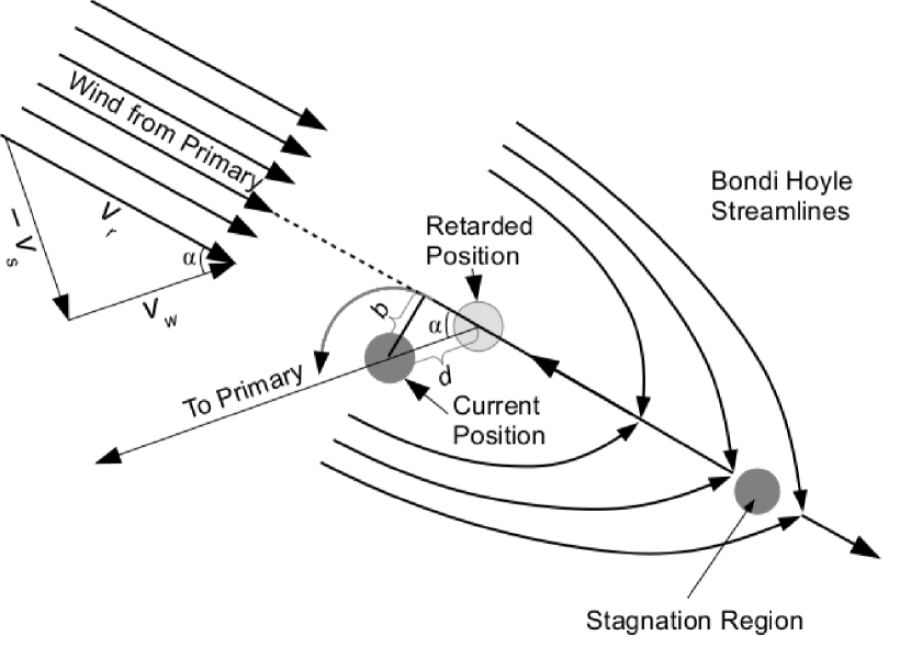
Figure 1: Schematic showing the flow structure of the binary wind capture process. The figure is in the inertial frame of the secondary and the direction of the motion of the primary is to the top left. The unlabeled curved arrow indicates the accretion column bending around the secondary and forming a disk.

The time scale, $t_{c}$, associated with the wind capture process scales approximately with the time scale for material to flow through the BHL radius, that is $t_{c}=\frac{r_{b}}{v_{r}}=\frac{2Gm_{s}}{v_{r}^{3}}$, where (again) $v_{r}$ is the velocity of the gas relative to the companion. In an inertial frame moving with the secondary’s velocity at $t_{0}$, the flow resembles a classical BHL pattern, although the secondary is accelerated from rest toward the primary with $a_{c}=\frac{v_{s}^{2}}{r_{s}}$. The distance, $d$, travelled by the secondary during the wind capture time scale $t_{c}$ is

$$d=\frac{1}{2}a_{c}t_{c}^{2},$$ (2)

and the distance perpendicular to the accretion column, is

$$b=d\sin{\alpha}=d\frac{v_{s}}{v_{r}}.$$ (3)

We call $b$ the accretion line impact parameter which can be expanded as

$$b=\frac{1}{2}\frac{v_{s}^{2}}{r_{s}}\left(\frac{2Gm_{s}}{v_{r}^{3}}\right)^{2}\frac{v_{s}}{v_{r}}=\frac{2G^{2}m_{s}^{2}v_{s}^{3}}{r_{s}v_{r}^{7}}.$$ (4)

Solving for $v_{s}$ and $r_{s}$ in terms of the mass of the primary, $m_{p}$, the total mass, $M=m_{s}+m_{p}$, and the total separation, $R$, we get

$$b=2\left(\frac{m_{s}^{2}M^{3}}{m_{p}^{5}}\right)\frac{\left(\frac{1}{R}\right)^{5/2}}{\left(\frac{1}{R}+\frac{1}{r_{w}}\right)^{7/2}}$$ (5)

where $r_{w}=\frac{Gm_{p}^{2}}{Mv_{w}^{2}}$ which for our choice of wind velocity and masses gives the profile in Figure 2.

We note two important points. First, the expression for (5) is valid only for timescales short enough for the frame to be considered inertial. Thus our expression for the accretion line impact parameter only holds for timescales short compared to the orbital time ($t<<P$, where $P$ is the orbital period). This is also the same limit as $d<<R$. Taken together these limits also imply our expression is only valid when the orbital separation $r_{s}$ is greater than the Bondi-Hoyle radius $r_{b}$.

In addition we note that our model implementation (section 3) assumes that the wind experiences a balance of radiation pressure and gravitational forces from the primary. This is equivalent to assuming the secondary orbits beyond the wind’s acceleration zone. Operationally this means a differential acceleration between the wind and the secondary occurs since the secondary does feel the full gravity from the primary. It is this differential acceleration which creates the accretion line impact parameter. We note however that even in the wind acceleration zone the radiation pressure force on the gas (but not on the secondary) would produce such a differential gravitational acceleration.

Finally we note that characterizing the appropriate “disk formation” radius in the context of Bondi-Hoyle flow in binaries is nontrivial. Different approaches have been used by different authors (Wang, 1981). For example, when considering flows with density gradients of scale $H$, Soker & Livio (1984) used earlier results by Dodd & McCrea (1952), and derived an expression for disk formation radius to be $r_{k}=GM/v^{2}(r_{b}/2H)^{2}$. In another work, Soker & Rappaport (2000) compared the angular momentum of accreted material through the Bondi-Hoyle radius $j_{a}$ to that of material in Keplerian orbit around the accretor $j_{2}$ such that $j_{2}<j_{a}$ for a disk to form. This expression can also be used to derive an expression for a disk formation radius $r_{a}$. We find that our expression for the accretion line impact parameter $b$ will, in the region of its validity, be larger than both these radii. This indicates that $b$, again in its domain of validity, defines the appropriate disk formation radius.

Figure 2: Plot showing the accretion line impact parameter as a function of separation for a 1.5 M_⊙ primary, a 1 M_⊙ secondary and a wind with terminal speed of 10 km s^-1.

One of the primary and novel results of the simulations that we present here is showing that accurately resolving this physical scale in the vicinity of the secondary is essential to capturing the dynamics of the flow. Since the material initially goes into orbit around the secondary with a radius of $b$, a failure to resolve the scale can lead to the lack of an accretion disk forming or the formation of disk with unphysical dynamics such as extreme warps or tilts.

3 Computational Methodology

To model the formation and evolution of disks in binary system, we use the adaptive-mesh-refinement (AMR), magnetohydrodynamical code AstroBEAR2.0. AstroBEAR is a highly-parallel, second-order accurate, shock-capturing, multi-physics Eulerian code (Cunningham et al., 2009; Carroll-Nellenback et al., 2011). While AstroBEAR2.0 has options for MHD, self-gravity and heat conduction, we neglect these processes in our current study.

We use BlueHive –an IBM massively parallel processing supercomputer of the Center for Integrated Research Computing of the University of Rochester– and Ranger –a Sun Constellation Linux Cluster which is part of the TeraGrid project– to run simulations for an average running time of about 0.5 days$/$orbit using 64-1024 processors.

We perform calculations in three-dimensions and solve the equations of hydrodynamics in a co-rotating frame, which in conservative form are:

$$\begin{array}[]{l l}\frac{\partial\rho}{\partial t}+\nabla\cdot(\rho\mbox{\bf v})&=0\\ \frac{\partial\left({\rho\bf v}\right)}{\partial t}+\nabla\cdot\left(\rho{\bf vv}\right)&=-\nabla p-\rho\nabla\Phi-2\rho\Omega\times{\bf v}\\ {}&\quad-\rho\Omega\times\left(\Omega\times{\bf r}\right)\end{array}$$ (6)

where $\rho$, $p$ and v are the gas density, pressure and flow velocity, respectively. The last two terms in the right hand side of equation (6) account for the centrifugal and the Coriolis forces that act on the gas. We employ an isothermal ideal gas equation of state with an adiabatic index of $\gamma=1$.

We follow the secondary star as it orbits about the system’s center of mass with a circular trajectory due to the gravitational field of the binary system. However, the gravitational effects that the stars have on the gas is modelled to be caused by the secondary star only. Thus we assume that there is a balance between the gravitational potential of the primary star and the wind radiation pressure (Section 3.1.3). The gravitational potential of the secondary star which affects the gas is computed using the functional form $\Phi=Gm_{s}/r$ for $r\geq 4\sqrt{dx^{2}+dy^{2}+dz^{2}}$, and we use a spline softening function at smaller radii.

3.1 Initial Conditions and Set-up

Our computational domain consists of a rectangular volume of 10x10x5 AU³. We employ a fixed grid of 64x64x32 base cells plus three, or four (see Table 1), AMR levels of factor two refinement. Nested refined cell blocks are centered at the secondary’s position such that the finest level has 32-64 cells (on the orbital plane) enabling us to resolve the central part of the disks and $b$ (section 2). We note that in our implementation the primary star is located outside the computational domain (see Figure 3, top).

We employ either wind boundary conditions (section 3.1.3) in the $-x,+y$ and $\pm z$ domain faces, or outflow only conditions in all other faces (Figure 3). We include Coriolis and centrifugal terms and use a reference frame which co-rotates with the secondary.

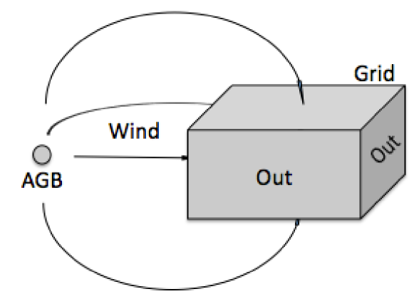
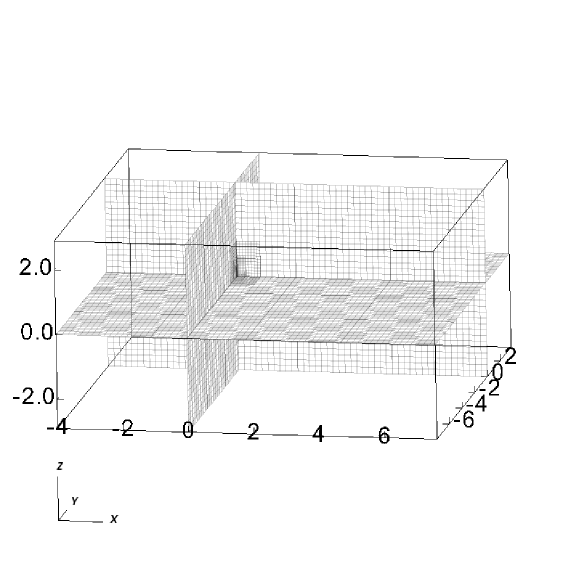
Figure 3: Top: Diagram showing the wind model and the grid. Bottom: Grid, its coordinates, in AU, and the central mesh. The secondary is located at the origin.

3.1.1 Primary

We use a simple AGB star model for the primary consisting of a mass of 1.5 M_⊙ and a wind with an isotropic velocity of $v_{w}=\,$10 km s^-1 and mass-loss rate of $\dot{m}_{p}=\,$10^-5 M_⊙ yr^-1. These values are typical for AGB stars (e.g. Hrivnak et al., 1989; Bujarrabal et al., 2001).

We note a few aspects of this model. First, winds from AGB stars are driven by radiation pressure acting on dust grains. Such interactions are complicated and many details depend subtle non-linear effects (Sandin & Höfner, 2003, and references therein). Additionally, observations suggest that AGB-star winds possess acceleration zones in which the radial wind velocity climbs slowly to its final value (e.g. see Sandin, 2008). Such acceleration regions may play a role in the formation of disks in binaries with separations $\la$ 10 AU. We expect this effect to be mild for the separations explored here (10-20 AU), thus no acceleration region has been considered and we leave more realistic AGB star wind models for future work. Additionally, we note that the binary separations that we explore here are outside the wind-Roche-lobe-overflow (WROLF) limit (Sandin, 2008; Mohamed & Podsiadlowski, 2011).

3.1.2 Companion

We model the secondary star using a sink particle, based on the implementation of Krumholz et al. (2004), which accretes gas within a radius of 4 grid cells. The mass, momentum and energy of the gas within this region are then acquired by the secondary in a conservative fashion. We set the secondary with an initial mass of 1 M_⊙ in a circular orbit about the primary. While important at these radii, we do not adjust the orbit for the effect of mass loss or tidal interactions as they occur on longer evolutionary timescales (Nordhaus et al. 2010; Nordhaus & Spiegel 2012; Spiegel & Madhusudhan 2012).

3.1.3 Wind solution and injection

We set the initial conditions throughout the grid with a constant temperature of 1000 K and a density given by

$$\rho_{w}=\frac{\dot{m}_{p}}{4\pi({\bf x}_{p}-{\bf x})^{2}v_{w}},$$ (7)

where $\dot{m}_{p}=\,$5$\times\,$10^-5 M_⊙ yr^-1, $v_{w}=\,$10 km s^-1, ${\bf x}_{p}$ and ${\bf x}$ are the positions of primary’s orbit and that of an arbitrary grid cell relative to the center of mass, respectively. We calculate the velocity field of the solution by solving for the characteristics that leave the surface of the primary at a retarded time, $t_{r}=t-|{\bf x}|/v_{w}$, with a velocity vector pointing towards ${\bf x}$. Wind speeds are chosen so that $v_{w}>|{\bf v}_{s}|$, where ${\bf v}_{s}$ is the secondary’s orbital velocity. We assume that the distance from the primary’s surface to ${\bf x}$ is larger than $|{\bf x}_{p}|$, which constrains the separation between the secondary and the grid’s boundaries. The wind that arrives at point ${\bf x}$ at the current time $t$ left the primary’s surface at a retarded time $t_{r}$. The vector connecting the primary’s retarded position and our current position ${\bf x}$ is given by

$${\bf d}={\bf x}-{\bf x}_{p}(t_{r}).$$ (8)

At any point on the primary, the wind velocity field, ${\bf u}={\bf u}({\bf x},t)$, is given by

$${\bf u}=v_{w}{\bf\hat{n}}+{\bf v}_{p}(t_{r}).$$ (9)

The vectors ${\bf u}$ and ${\bf d}$ should be parallel at $t_{r}$ –when ${\bf u}$ left the primary’s surface, i.e.

$$(v_{w}{\bf\hat{n}}+{\bf v}_{p}(t_{r}))\times{\bf d}=0.$$ (10)

We can then solve for ${\bf\hat{n}}$ and the wind vector at the retarded time. A better approximation of the retarded time is then found using ${\bf u}$:

$$\tau_{r}=t-|{\bf x}|/|{\bf u}|.$$ (11)

We iterate the above computations until we find a convergent wind solution for the gird cell located at ${\bf x}$. Finally, we transform the solution to a reference frame which co-rotates with the secondary.

Once the initial conditions are set, we continually give the above wind solution to the grid cells in the $-x,+y$ and $\pm z$ domain faces (Figure 3, top). For each iteration however we use $\tau_{r},\,{\bf x}_{p}(\tau_{r})$ and ${\bf u}$ as initial conditions in a recursive Runge-Kutta method to calculate the deflection of ${\bf u}$ –as it travels from the primary’s surface [$\sim\,{x}_{p}(\tau_{r})]$ to ${\bf x}$– caused by the secondary’s gravity field. We consider the orbital motion of the secondary in these computations. This step yields yet better estimates of both ${\bf\hat{n}}$ and $\tau_{r}$ than the calculations in equation (9) alone. We therefore use the new values of ${\bf\hat{n}}$ and $\tau_{r}$ for the next iteration of the wind solution.

Finally, to match the initial conditions and the injected wind solution we allow the gravitational effect that the secondary has on the gas to increase linearly during one wind crossing time, 1.6 $r_{b}/v_{w}$, from zero to $Gm_{s}/r$. The field remains constant thereafter. This has no effect on the binary orbital motion.

4 Results

We carry out three simulations corresponding to stellar separation of 10, 15 and 20 AU. Table 1 summarizes the models and their relevant parameters.

Table 1: Simulations and parameters.

Name	Separation [AU]	Resolution	$r_{b}$ [AU]	$b$ [AU]
M1	10	64x64x32+3amr	4.9	2.4
M2	15	64x64x32+4amr	5.8	1.5
M3	20	64x64x32+4amr	6.3	1.0

$\log{(n)}$ [part cm^-3]                                Flow speed [Mach]

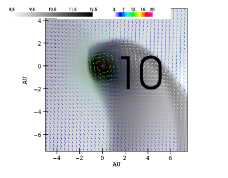
                   Face-on:
 
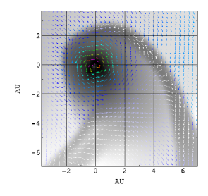
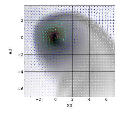
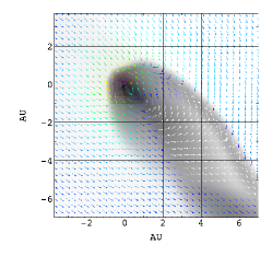
              Face-on, zoom in:
   
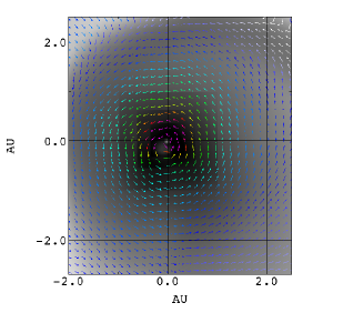
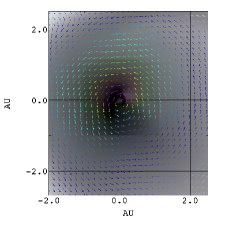
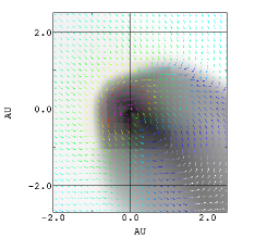
       Edge-on:

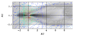
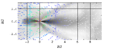
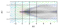
Figure 4: Logarithmic density gray-scale and velocity field maps for the 10 AU (left), 15 AU (middle) and 20 AU (right) models at $t=\,$3 orbits. The primary is simulated to be to the left of the maps. The secondary is receding in bottom row panels due to its orbital motion.

4.1 Disk structure and formation

In order to present the main results of our study in Figure 4 we show logarithmic density gray-scale and velocity field maps of our three simulations at $t=\,$3 orbits. Rows 1 and 2 of Figure 4 show slices though the orbital plane (at two different scales), while the bottom row shows slices though a longitudinal plane that intersects the secondary. These density maps allow us to see the large scale structure of the flows and to compare those flows as the orbital separation is increased.

First we note the basic BHL converging flow which can be seen in bottom row of Figure 4. The AGB wind can be seen streaming in from the left and is subsequently focused towards the midplane by the gravitational force of the secondary. At the time of these images the global flow is considerably more complicated than that described by the simple BHL scenario, however, because of the presence of fully formed accretion disks. Thus, as Figure 4 makes clear, accretion disks are created in all our simulations. These disks form, as expected, from the BHL accretion stream that originates at the stagnation region (below) downstream from the secondary.

We provide a better illustration of the stagnation region in Figure 5 where the top panel shows iso-surfaces of the disk’s density and slow material’s velocity. The middle panel shows one wind flow streamline which starts at the boundary, is deflected by the secondary’s gravity field, reaches the stagnation region then, and is finally accreted onto the disk. In the bottom panel we show several flow streamlines from a different perspective using a velocity color table that clearly shows the stagnation region structure. We note the appearance of nested flow surfaces, whose areas increase with distance from the stagnation region. Thus the accretion column resembles a strong vortex tube –instreaming material flowing along helical paths towards the secondary star– and our simulations are the first to capture this aspect of BHL flows in binaries.

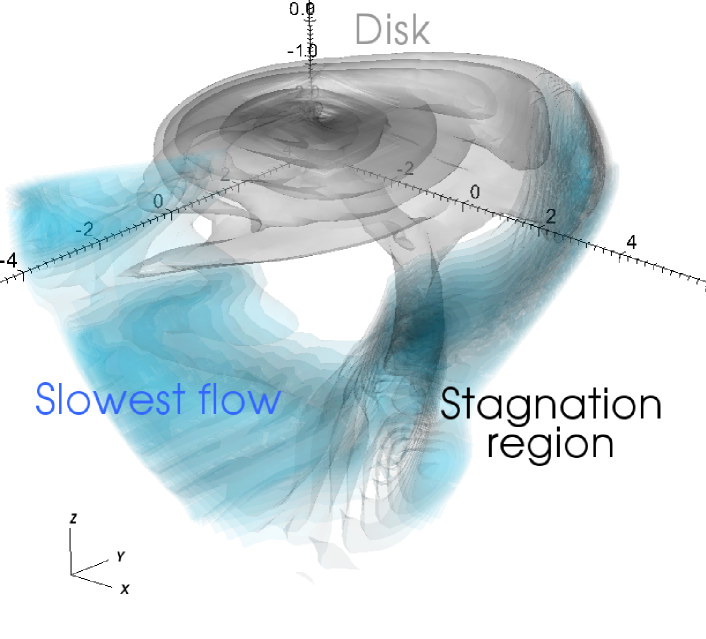
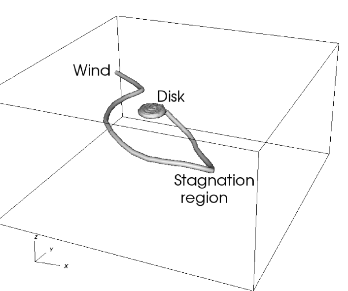
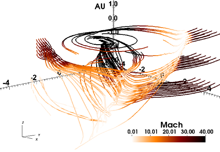
Figure 5: Structure of the stagnation region for the 15 AU case at $t=\,$3 orbits. Top: gray shows disk density iso-surfaces, while blue shows velocity iso-surfaces of wind material with speeds $<$2 km s^-1. Middle: flow streamline that starts at the boundary (wind), is deflected by the secondary’s gravitational field, reaches the stagnation region and is finally accreted onto the disk. Bottom: flow streamline field with a color scale in Mach units.

The density maps in both the equatorial and perpendicular planes (Figure 4) also reveal the presence of bow shocks around the accretion disks. Such shocks also form in the classic BHL flow however once the disks emerge, incident AGB wind must stream around them creating more complex post-shock flow patterns. The velocity vectors in the upper row panels of Figure 4 are of particular interest, showing the redirection of high density flow behind the bow shock and its interaction with the counterstreaming flow in the accretion disk.

To understand the structure and evolution of the disks more explicitly, in Figure 6 we show logarithmic density contours of the disk in slices though the orbital and perpendicular planes. Each panel has 12 contours arranged by line type and color: blue, red and black represent densities of (3.5, 10.5, 35) $\times$10¹⁰ part cm^-3, respectively. Dashed, dotted and dashed-dotted lines represent densities at $t=\,$1, 2 and 3 orbits, respectively.

The density contour maps for different orbital separations are mutually consistent in terms of evolutionary stages but are correspondingly different with respect to the time scales and some features of these phases. Comparing contours of the same color (Figure 6) we see a given iso-density structure at different evolutionary times. These show that once the disk forms further structural changes are mild. Thus in all cases the disks begin ($t=\,$0.1) from long elliptical structures that can be identified as the curved BHL accretion stream. By ($t=\,$1.0) the inner regions of the disk have formed and we see well defined inner black contours which do not change appreciably with time. The middle and outer contours in all three case (red and blue) do show some evolution after $t=\,$1.0. However, these changes tend to be higher order in morphology, whereas overall shape (circular in the $a=10$ and $15$ AU case and elliptical in the $a=20$ AU case) and radii do not change.

Comparing the solid lies in left panels we find, in agreement with the discussion in section 2, that the angle between the accretion flow and the wind decreases with increasing orbital separation, $a$. This angle is close to zero already in the 20 AU model. Thus, as expected, the solution (4) converges to the BHL one for large separations.

We note that given our choice of $\gamma=1$, the accretion disks which form in our models are thin which is consistent with a low gas temperature and sound speed ($h/R\sim c/\Omega)$. The disks orbits are also not circular. We see orbits with eccentricities $e>0$ in all cases, however the magnitude of the average eccentricity increases with increasing orbital separation. And while our disks are thin, we do see flared vertical structures that are also not symmetric in the ($r,z$) plane of the disk but larger on their downstream side relative to the wind. The effect of the wind on the disk is also apparent in that the steepest density gradients are located where the disks impinge on the incoming stellar flow (top left region in left panels and left region in right panels, Figure 6). We find that both the disks’ outer radius, $r_{d}$, and edge height are inversely proportional to $a$. In section 4.3 we show that the shape of the gas parcel orbits in the disk is a function of $a$ as well. We note that the disks’ inclination angles are generally small, meaning that the disks are close to perpendicular to the orbital plane. However, small time variation in the flow occur even after the disks settle into a quasi-steady state.

4.2 Disk mass

In Figure 7 we show profiles of the disks’ mass, $M_{d}(t)$ (solid lines), as a function of both time and the binary separation. These are calculated by summing the mass of grid cells containing bound gas (those having a gravitational energy greater than the kinetic one).

In the 10 AU case we see that the disk mass increases during the first orbit and then saturates at about 7$\times$10^-6 M_⊙. The disk mass then oscillates with a period of $\sim\,$1 orbit and an amplitude of about 1$\times$10^-6 M_⊙.

To understand the origin of these disk mass oscillations, we calculate the gas flux leaving the grid though both the $+x$ and $-y$ boundaries (see Figure 3) in M_⊙ yr^-1 (dashed lines, Figure 7). The position and shape of the gradients in $M_{d}(t)$ compared with those of the mass fluxes indicate that the disk’s mass decreases with increasing outbound flux and vice versa. This suggests the wind’s post bow shock ram pressure mediates the disk mass; the wind appears able to strip a small fraction of disk’s gas and liberate it from the gravitational pull of the companion. This is likely to happen at the outer parts of the disk where the ram pressures of the wind and the disk are comparable. Thus the wind-disk interaction induces perturbations on the orbits of the disk material, which may be sufficiently strong to overcome the gravitational potential of the companion. Some disk gas is pushed outside the computational domain then.

Moving to comparisons of simulations with different $a$, we see that the disk mass in the 15 AU model reaches its maximum value of about 4$\times\,$10^-6 M_⊙ in $\sim\,$0.7 orbits (earlier than the $a=10$ AU case). Once again we see disk mass oscillations with amplitudes of about 1$\times\,$10^-6 M_⊙ and a frequency of $\sim\,$0.3 orbits. Note that these oscillations have a smaller amplitude and period than for the 10 AU case. This would be consistent with our wind stripping interpretation as the wind’s ram pressure is proportional to $a^{-2}\,{\bf x}_{s}^{-1}$, where ${\bf x}_{s}^{-1}$ is the distance between the secondary and the center of mass.

The disk mass profile of the 20 AU model is quite different. While an initial disk forms with a mass $\sim\,$6.5$\times$10^-7 M_⊙, a sharp growth in mass is seen at $t\approx\,$0.85 orbits. The increase occurs in less than $0.1$ of an orbit ($t=5.5\,yr$) and the disk mass then reaches a maximum value of $\sim\,$6.5$\times$10^-7 M_⊙ after a brief period of relaxation. Note that in this case we do not see any disk mass oscillations. This behavior is also consistent with our wind stripping interpretation as the model wind ram pressure is the weakest at 20 AU away from the primary.

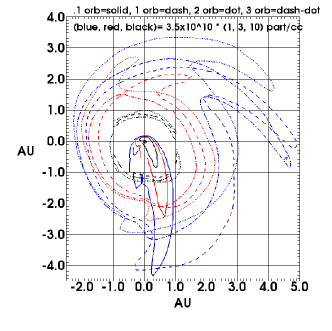
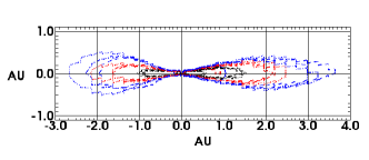
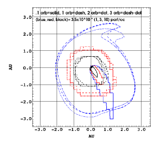
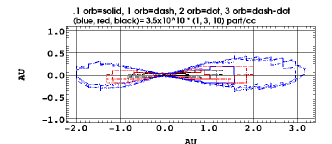
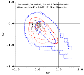
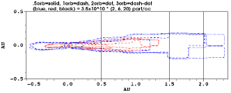
Figure 6: Disk density structure at 4 times. Left: face-on view where the wind enters the grid from the top left corner at an angle close to 45^∘ and the secondary orbital motion is upwards. Right: edge-on view where the wind enters the grid horizontally from the left side and the secondary is receding due to its orbital motion. The primary is simulated to be to the left of all maps. Top, middle and bottom rows correspond to binary separations of 10, 15 and 20 AU, respectively.

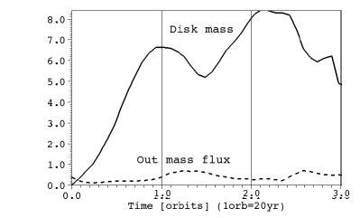
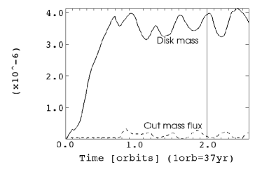
(a) $a=\,$10 AU                                                     (b) $a=\,$15 AU

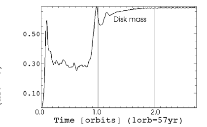
(c) $a=\,$20 AU

Figure 7: Disk mass as a function of time [M_⊙] (solid) and flux of gas that leaves the grid [M${}_{\odot}\,$yr^-1] (dashed).

4.3 Disk orbits

An interesting result from our simulations is that the shape of the disk gas orbits significantly depends on $a$. We show this relation using the disk gas streamline maps in Figure 8, where the top panel presents a 3-D map of the disk gas velocity distribution in colors for the 10 AU model, along with sliced (half the disk) density contours in translucent red color. The lines show that the gas is supersonic, the orbits have low eccentricities, $e$, and the velocity decreases with distance from the secondary.

In the bottom row of Figure 8, we show a quantitative comparison of disk gas orbits as a function of $a$, at $t=\,$3 orbits, corresponding to the 10, 15 and 20 AU cases from left to right, respectively. The maps consistently show that $e$ is a function of both, $r_{d}$ and $a$. For a particular disk, material located at small disk radii shows moderately higher $e$ than material located at larger radii. Comparing disks with different $a$ we see that (i) the magnitude of the average $e$ increases with increasing $a$ and (ii) the angle between the semi-major axis of the orbits and the wind velocity field decreases with $a$. The latter is particularly clear in orbits with small disk radii. This behaviour is in good agreement with our findings in section 6; the angle is close to zero in the 20 AU model (right-most panel).

Finally, the color bars in the bottom panels of Figure 8 show disk gas position along the direction perpendicular to the orbital plane; receding material is red whereas approaching material is blue. Note that we have chosen different color limits in each panel in order to stress disk orbital features. The color of the lines in the 10 and 15 AU cases (left and middle panels) consistently shows that material oscillates about the orbital plane mildly with amplitudes no larger than 0.2 disk radii and frequencies of order half an orbit. The oscillation are much weaker in the 20 AU case. We do not see any correlation between the color of the lines –i.e. the position about the orbital plane– and the wind velocity field direction (which points from the top left corner to the bottom right one; Figure 8 bottom row).

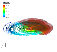
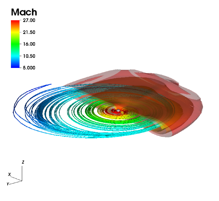
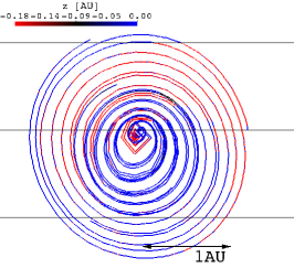
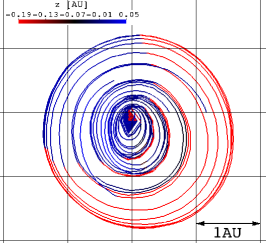
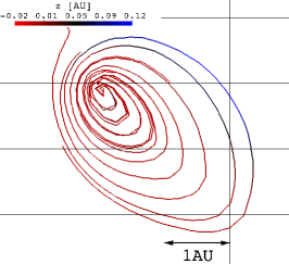
Figure 8: Top: 3-D disk gas orbit streamlines and sliced density contours (red) for the 10 AU case at $t=\,$2 orbits. The central white small sphere is the secondary. Streamline colors denote orbital speed in Mach units. The wind enters the grid towards the image. Bottom: Disk gas orbit streamlines at $t=\,$3 orbits corresponding to the 10, 15 and 20 AU cases, from left to right. The wind enters the grid from the top left corner moving towards the bottom right. Colors denote distance perpendicular to the orbital plane in AU and indicate the orbits inclination.

5 Discussion

5.1 Accretion onto the companion and implications for PPN/PN phenomenology

In Figure 9, we show the evolution of the secondary’s accretion rate. The plots show the total gas flow into a region within a 4 cell radius from the star’s center (section 3.1.2) as a function of time. The plots demonstrate that after a steep initial increase which lasts for about 0.05 orbits the accretion rate reaches a quasi-steady value with oscillations of a period that decreases with $a$. These accretion histories are consistent with those of de Val-Borro et al. (2009, see their Figure 12). We note that we see a small dip in the 20 AU profile, close to 0.9 orbits, which corresponds to the disk formation time.

The analytic Bondi-Hoyle accretion rate for a high velocity wind and negligible pressure conditions is given by

$$\dot{m}_{BH}=\pi R_{b}^{2}\rho({\bf x}_{s})\sqrt{v_{w}^{2}+v_{s}^{2}},$$ (12)

where $R_{b}=\,$2$Gm_{s}\,(v_{w}^{2}+v_{s}^{2})^{-1}$ is the modified BHL radius (Edgar, 2004). For our 10, 15 and 20 AU models, $\dot{m}_{BH}$ takes the values of 3.3, 1.8 and 1.2$\times\,$10${}^{-6}\,$M${}_{\odot}\,$yr^-1, respectively. Thus the secondary accretion rates we find in Figure 9 (0.85, 0.5 and 0.3$\times\,$10${}^{-6}\,$M${}_{\odot}\,$yr^-1, for $a=\,$10, 15 and 20 AU, respectively) are $\dot{m}_{10AU}\sim\,$0.26$\dot{m}_{BH,10}$, $\dot{m}_{15AU}\sim\,$0.28$\dot{m}_{BH,15}$ and $\dot{m}_{20AU}\sim\,$0.25$\dot{m}_{BH,20}$, where the subscripts: $BH,10;BH,15;BH,20$ indicate the Bondi accretion rates at $10,15$ and $20$ AU.

Our results appear to be consistent with those found by other authors. For example in the models of de Val-Borro et al. (2009), the one with $a=\,$70 AU produced $\dot{M}_{acc}/\dot{M}_{wind}\sim$0.06 after 2 orbits. While we have not run any simulations with such a large orbital separation, these values are in line with the trend we observe in our results. The semi-analytic models of Perets & Kenyon (2012) yield $\dot{m}$ values that are also consistent with ours. For example their Model 2 with $a=10$ AU, $m_{p}=\,$3.0 M_⊙, $m_{s}=\,$1.0 M_⊙ and ${\dot{M}}_{p}=\,$10^-5 M_⊙ y^-1 yielded $\dot{M}_{acc}\sim\,$3$\times$10^-7. We note that the models of Perets & Kenyon (2012) are semi-analytic, therefore a direct comparison between our work and theirs is not straightforward.

The formation of these disks depends on the specific angular momentum of the accreted mass, $j_{a}$ (Soker & Rappaport, 2000). It is important to consider $j_{a}$ relative to the analytic net specific angular momentum of wind material that enters $r_{b}$, $j_{BH}$, which is given by

$$j_{BH}=\frac{1}{2}(\frac{2\pi}{P})r_{b}^{2},$$ (13)

where $P$ is the orbital period. Our models show that $j_{a}/j_{BH}(a=\,$10)$=\,$0.35/2.52$=\,$0.13, $j_{a}/j_{BH}(a=\,$15)$=\,$0.35/1.89$=\,$0.18 and $j_{a}/j_{BH}(a=\,$20)$=\,$0.30/1.47$=\,$0.20. Here, we computed the numerators using the accreted gas and calculating a representative average value of the $z$ component (perpendicular to the orbital plane) of the cross product given by the radial distance from the secondary’s center times the gas velocity. These figures are slightly higher, yet sensibly close, to analytical estimates of the specific angular momentum of isothermal high Mach number flows, for which $j_{a}/j_{BH}\simeq\,$0.1 (Livio et al., 1986; Ruffert, 1999).

The results shown in Figure 9 are relevant for constraining the class of models that can power PN outflows and, in particular, the PPN outflows in the reflection nebulae thought to precede the PN phase. The observations of Bujarrabal et al. (2001) imply that statistically, many PPN seem to harbor very powerful outflows whose energies and estimated acceleration times give mechanical luminosities as high as 4 $\times$ 10³⁶ erg s^-1 (Blackman 2009, see also Huggins 2012). Can the accretion rates we find power such high luminosities?

If these high powered PPN outflows do indeed result from accretion disk around a secondary, then one typically expects no more than 10% of the accretion rate to turn into mass outflow and the outflow speed to be $\Omega r_{A}=Qv_{K}$ (e.g. Frank & Blackman 2004), where $\Omega$ is the orbital speed at the inner edge of the disk, $r_{A}$ is the radius of the Alfvén surface, $v_{K}$ is the Keplerian speed at that radius and $Q$ is a numerical factor determining the jet speed as a multiple of the Keplerian speed (if the jet propagated into a vacuum). Although PPN jets would propagate into the stellar envelope such that the observed jet speed would be reduced using momentum conservation (Blackman 2009), the mechanical luminosity of the jet should be comparable to its naked value if energy is conserved in the outflow. Accretion would provide a jet mechanical luminosity of

$$\begin{array}[]{l l}L_{j}&\sim{1\over 2}{{\dot{M}}_{ac}\over 10}Q^{2}v_{K}^{2}\\ {}&=4\times 10^{36}\left({M_{ac}\over 5.6\times 10^{-5}{M_{\odot}/{\rm yr}}}\right)\left({Q\over 3}\right)^{2}\left({v_{K}\over 440{km/s}}\right)^{2},\end{array}$$ (14)

where we have scaled $v_{K}$ to that of an orbit at the surface of a main sequence star of 1 $M_{\odot}$ and 1 $R_{\odot}$ and taken an optimistic $Q=\,$3. The accretion rates we find (see Figure 9) would then fall short by $\sim\,$2 orders of magnitude if the secondary is a main sequence star. However, for a white dwarf, $v_{K}^{2}$ is $\sim\,$70 times larger and the required accretion rate to produce the same mechanical luminosity is reduced by the same factor, and becomes 8 $\times$ 10^-7 M_⊙ yr^-1. This rate is not that dissimilar from the accretion rate we found for the 10 AU separation case. Note that the estimates above depend on the value of $Q$ which is somewhat uncertain and on the actual inner most radius of the disk used to compute $v_{K}$. It could be that the disk does not extend all the way to the star in which case $v_{K}$ in the above formula would be reduced.

Figure 9: Secondary accretion rate evolution.

The fact that only a white dwarf companion could supply the outflow powers for the highest powered PPN, highlights the need to determine the mechanical luminosity distribution function of PPN. If the highest outflow powers are much more common than the expected frequency of white dwarf companions within 10 AU then the required mechanism would likely require closer binary interactions and perhaps even common envelope evolution. More work is needed to assess the various modes of accretion that can operate within a common envelope, either onto the primary, or onto the secondary (Nordhaus & Blackman, 2006; Nordhaus et al., 2011). It should be noted that the late stage PN are less demanding with respect to required accretion rates than the early PPN objects and it may be that not all PPN are as demanding as the Bujarrabal et al. (2001) sample.

One example of a lower power object of interest is the Red Rectangle PPN. In fact this object, reported in Bujarrabal et al. (2001), is one of the lower powered PPN presented therein. Witt et al. (2009) showed that the Red Rectangle is consistent with accretion onto a main sequence companion at binary separation $<$1 AU. The jet has a mechanical luminosity $\sim\,$ 7$\times$ 10³³ erg s^-1. Witt et al. (2009) plausibly argue from presumed evidence for disk emission that the disk around the companion is accreting via Roche lobe overflow from the primary at a rate 2–5$\times$ 10^-5 M_⊙ yr^-1. However, these authors argue that the jet outflow speed would be launched at 100 km s^-1 given this accretion rate, which is significantly below the escape speed at the inner edge of the disk if the disk were to extend all the way to the star. Such an accretion rate could certainly power the observed jets in the Red Rectangle.

In the future, a larger parameter survey covering a systematic range of grid resolution setups and accreting radii about the secondary (sink particle) –gravity softening radii– would be helpful both, to further constrain the connection between core accretion and jet launch in binary-formed disks and to better characterize numerical artifacts.

6 CONCLUSIONS AND SUMMARY

We have performed the highest resolution simulations to date of wind accretion and disk formation in an evolved star binary system. We simulated the wind accretion process at three different orbital radii, 10, 15 and 20 AU, and found accretion disk formation in all cases. We have also derived an accretion line impact parameter criterion that determines the minimum required resolution for such simulations to produce physically consistent results.

In our derivation we assume the wind experiences a balance of radiation pressure and gravitational forces from the primary. This is equivalent to assuming the secondary orbits beyond the wind’s acceleration zone. Operationally this means a differential acceleration between the wind and the secondary occurs since the secondary does feel the full gravity from the primary. It is this differential acceleration which creates the accretion line impact parameter. We note however that even in the wind acceleration zone the radiation pressure force on the gas (but not on the secondary) would produce such a differential gravitational acceleration.

The accretion line impact parameter $b$ measures the perpendicular (retarded) distance from the stagnation point in the BH accretion stream to the accretor and as such is a measure of the distance at which material from the wind is captured into orbit around the secondary. We have compared the validity of this parameter to other formulations of a “disk formation” radius and found that in the regime of applicability $b$ is the larger of the expressions and hence represents the outer most distance at which a disk will form.

Additionally, accretion disks formed in our simulations at 10 and 15 AU incur mass oscillations which appear to result from ram pressure stripping of the outer disk radii. The 15 AU oscillations become weaker as the wind ram pressure decreases with orbital radius (due to the wind density’s $r^{-2}$ density profile (7). The 20 AU disks, showed no oscillations, consistent with an even weaker wind ram pressure.

The disk accretion rates evolve to be quasi-steady after 1$/$4 orbits. The accretion rates are lower for larger orbital radius, taking values 8, 5 to 3 $\times$10${}^{-7}\,$M${}_{\odot}\,$yr^-1, for the 10, 15 and 20 AU cases, respectively. We note that for the secondary’s mass that we explore here, the simplest version of Bondi-Hoyle accretion model (steady uniform parallel wind flow) only applies truly at large separations; only in such cases is the angle between the accretion flow and the wind zero. We see this angle becoming $<\,$5^∘ for the 20 AU case, but it is non-negligible for the smaller radii runs.

While the basic problem of accretion from a wind studied herein has broad applicability in a number of contexts, we chose the parameters to be consistent with those of a stellar mass companion accreting from an AGB wind. This is motivated by the need to identify constraints on the mode of accretion that might be needed to explain the accretion powered jets and outflows of PPN and PN. Toward this end, we find that the accretion rates from our simulations fall short of what is needed to be able to power the most powerful young bipolar PPN unless the companion is a white dwarf. Closer binary interactions, which includes common envelope evolution, are likely an important player for some PPN objects but; our present work focused only on binary radii at 10 AU and larger separation in order to be be largely outside of the radiative wind acceleration zone. It is useful to compare our work with other studies of wind capture accretion in binary systems. Theuns & Jorissen (1993) used SPH simulations and despite low resolution by today’s standards were able to capture the basic features of a bow-shock and disk formation. In the seminal work by Mastrodemos & Morris (1999) SPH methods were again used to systematically explore the formation of accretion disks. Their work implied that disks could form out to distances of at least 21 AU. Their 3-D models also hinted at the formation of significant warps in the disks which would be important as these might drive precession in any jets which form from the disks. The work of de Val-Borro et al. (2009) found disks forming out to radii of 70 AU. If such a result where to hold it would be important for establishing the population of binaries for which disk winds might power jets. Unfortunately the de Val-Borro et al. (2009) study was carried out in 2-D only so it not possible with our work to confirm their outer limits on disk formation. Of equal importance was the role of the inner AGB wind launching radius $R_{w}$ in their studies. de Val-Borro et al. (2009) allowed the inner wind launching radius to be a free parameter. The justification for this was the possibility of large wind acceleration zones for AGB stars. In their simulations de Val-Borro et al. (2009) found that as $R_{w}$ increased the flow pattern became more complex appearing as a mix between Roche Lobe overflow and wind capture. Such a mix of accretion modes was also implied by Mohamed & Podsiadlowski (2007). In Perets & Kenyon (2012) semi-analytic methods also found disks forming at large binary separations ($a=\,$100 AU). If these results can be verified in full 3-D fluid dynamical simulations they would also enlarge the population range of outflow bearing systems (though these outflows would likely be of low power as explained in the previous section). Taken as a whole, understanding these possibilities in greater detail will be essential for understanding the evolutionary pathways and outflow generation of PPN and PN systems.

Finally we note that our study provides new insights into the Bondi-Hoyle accretion in binary systems. We find for example that the stagnation region in which the accretion “line” separates into flows directed towards and away from the accretor is best viewed as a vortex tube as instreaming material flows along helical paths towards the secondary star. In addition we find the flows (and most important the disks) which form via binary BH flows appear quite stable (Blondin & Pope, 2009; Blondin & Raymer, 2012). Only small amplitude fluctuations in the orientation of different disk annuli are seen and these would appear to be too small to drive significant jet precession. In conclusion, more work is needed to explore the consequences of interacting binaries for a wider range of orbital radii. And more observations are needed to determine the mechanical luminosity function of PPN jets to assess what fraction have the high powered jets that are typical of the Bujarrabal et al. (2001) PPN sample.

References

- Balick & Frank (2002) Balick, B., & Frank, A., 2002, ARAA, 40, 439
- Blackman et al. (2001) Blackman, E. G., Frank, A., & Welch, C.,2001, ApJ, 546, 288
- Blackman (2009) Blackman, E. G., 2009, IAU Symposium, 259, 35
- Blackman & Nordhaus (2007) Blackman, E. G., & Nordhaus, J. T., 2007, Asymmetrical Planetary Nebulae IV
- Blackman (2007b) Blackman E.G., 2007, Ap&SS, 307, 7
- Blandford & Payne (1982) Blandford, R. D., & Payne, D. G. 1982, MNRAS, 199, 883
- Blondin & Pope (2009) Blondin, J.M., & Pope, T.C., 2009, ApJ, 700,95
- Blondin & Raymer (2012) Blondin, J.M., & Raymer, E. R., 2012, Apj, in press
- Bujarrabal et al. (2001) Bujarrabal, V., Castro-Carrizo, A., Alcolea, J., Sánchez Contreras, C., 2001, AAP, 377, 868
- Carroll-Nellenback et al. (2011) Carroll-Nellenback, J. J., Shroyer, B., Frank, A., & Ding, C., 2011, arXiv:1112.1710
- Cunningham et al. (2009) Cunningham A. J., Frank A., Varnière P., Mitran S., & Jones, T. W. 2009, ApJS, 182, 519
- De Marco (2009) De Marco, O. 2009, PASP, 121, 316
- D’Souza et al. (2006) D’Souza, M. C. R., Motl, P. M., Tohline, J. E., & Frank, J. 2006, Apj, 643, 381
- Dodd & McCrea (1952) Dodd, K. N., & McCrea, W. J., 1952, MNRAS, 112, 205
- Edgar (2004) Edgar, R., 2004, NAR, 48, 843
- Edgar et al. (2008) Edgar, R. G., Nordhaus, J., Blackman, E. G., & Frank, A. 2008, Apjl, 675, L101
- Eggleton (1983) Eggleton, P. P. 1983, Apj, 268, 368
- Hrivak et al. (1989) Hrivak, B. J., Kwok, S., Volk, K. M., 1989, ApJ, 346, 265
- Huarte-Espinosa et al. (2012) Huarte-Espinosa, M., Frank, A., Balick, B., et al., 2012, MNRAS, 424, 2055
- Huggins (2012) Huggins, P. J., 2012, American Astronomical Society Meeting Abstracts #219, 219, #239.01
- Huggins et al. (2009) Huggins, P. J., Mauron, N., & Wirth, E. A. 2009, MNRAS, 396, 1805
- Jahanara et al. (2005) Jahanara, B., Mitsumoto, M., Oka, K., et al., 2005, AAP, 441, 589
- Kim & Taam (2012) Kim, H., & Taam, R. E. 2012, arXiv:1209.2128
- Kim & Taam (2012) Kim, H., & Taam, R. E. 2012, Apj, 744, 136
- Krumholz et al. (2004) Krumholz, M. R., McKee, C. F., & Klein, R. I. 2004, Star Formation in the Interstellar Medium: In Honor of David Hollenbach, 323, 401
- Livio et al. (1986) Livio, M., Soker, N., de Kool, M., & Savonije, G. J., 1986, MNRAS, 222, 235
- Mastrodemos & Morris (1999) Mastrodemos, N., & Morris, M., 1999, Apj, 523, 357
- Mastrodemos & Morris (1998) Mastrodemos, N., & Morris, M., 1998, Apj, 497, 303
- Makita et al. (2000) Makita, M., Miyawaki, K., & Matsuda, T., 2000, MNRAS, 316, 906
- Mohamed & Podsiadlowski (2007) Mohamed, S., & Podsiadlowski, P., 2007, Asymmetrical Planetary Nebulae IV
- Mohamed & Podsiadlowski (2011) Mohamed, S., & Podsiadlowski, P., 2011, Why Galaxies Care about AGB Stars II: Shining Examples and Common Inhabitants, 445, 355
- Nagae et al. (2004) Nagae, T., Oka, K., Matsuda, T., et al., 2004, AAP, 419, 335
- Nordhaus & Blackman (2006) Nordhaus, J., & Blackman, E. G. 2006, MNRAS, 370, 2004
- Nordhaus et al. (2007) Nordhaus, J., Blackman, E. G., & Frank, A. 2007, MNRAS, 376, 599
- Nordhaus et al. (2010) Nordhaus, J., Spiegel, D. S., Ibgui, L., Goodman, J., & Burrows, A. 2010, MNRAS, 408, 631
- Nordhaus et al. (2010) Nordhaus, J., Spiegel, D. S. submitted to MNRAS Letters.
- Nordhaus et al. (2011) Nordhaus, J., Wellons, S., Spiegel, D. S., Metzger, B. D., & Blackman, E. G. 2011, Proceedings of the National Academy of Science, 108, 3135
- Ouyed & Pudritz (1997) Ouyed, R., & Pudritz, R. E. 1997, ApJ, 482, 712
- Perets & Kenyon (2012) Perets, H. B., & Kenyon, S. J., 2012, arXiv:1203.2918
- Ruffert (1999) Ruffert, M., 1999, AAP, 346, 861
- Sandin & Höfner (2003) Sandin, C., Höfner, S., 2003, AAP, 398, 253
- Sandin (2008) Sandin, C. 2008, MNRAS, 385, 215
- Soker & Livio (1984) Soker, N., & Livio, M., 1984, MNRAS, 211, 927
- Soker & Rappaport (2000) Soker, N., & Rappaport, S., 2000, Apj, 538, 241
- Soker & Rappaport (2001) Soker, N., & Rappaport, S. 2001, Apj, 557, 256
- Soker & Kashi (2012) Soker, N., & Kashi, A. 2012, Apj, 746, 100
- Spiegel & Madhusudhan (2012) Spiegel, D. S., & Madhusudhan, N., 2012, ApJ, 756, 132
- Struck et al. (2004) Struck, C., Cohanim, B. E., & Willson, L. A., 2004, MNRAS, 347, 173
- Theuns & Jorissen (1993) Theuns, T., & Jorissen, A., 1993, MNRAS, 265, 946
- de Val-Borro et al. (2009) de Val-Borro, M., Karovska, M., & Sasselov, D., 2009, Apj, 700, 1148
- Witt et al. (2009) Witt, A. N., Vijh, U. P., Hobbs, L. M., et al., 2009, Apj, 693, 1946
- Wang (1981) Wang, Y.-M., 1981, AAP, 102, 36