Bayesian Learning and Predictability in
a Stochastic Nonlinear Dynamical Model

Abstract

Bayesian inference methods are applied within a Bayesian hierarchical modelling framework to the problems of joint state and parameter estimation, and of state forecasting. We explore and demonstrate the ideas in the context of a simple nonlinear marine biogeochemical model. A novel approach is proposed to the formulation of the stochastic process model, in which ecophysiological properties of plankton communities are represented by autoregressive stochastic processes. This approach captures the effects of changes in plankton communities over time, and it allows the incorporation of literature metadata on individual species into prior distributions for process model parameters. The approach is applied to a case study at Ocean Station Papa, using Particle Markov chain Monte Carlo computational techniques. The results suggest that, by drawing on objective prior information, it is possible to extract useful information about model state and a subset of parameters, and even to make useful long-term forecasts, based on sparse and noisy observations.

Keywords: Bayesian Hierarchical Modelling, Data Model, Inference in Nonlinear Models, Prediction, Parameter (Prior) Model, Stochastic Process Model, Uncertainty

1 Introduction

The last century has seen major advances in the ecological and earth sciences, both in the development of theoretical understanding, encapsulated in mechanistic process models, and in the development of sophisticated statistical theories and models for the interpretation and analysis of observations. However, as Berliner (2003) has pointed out, until recently the development of process models and the statistical analysis of observations have occurred in parallel and somewhat at arms length. Over the last two decades, there has been increasing effort devoted to the integration of observations and process models, so that model–data comparison and data assimilation are now key research topics.

There are a number of drivers for this increased emphasis on the integration of models and observations. The scientific community increasingly insists on the use of more objective and quantitative measures or metrics to evaluate model predictions against observations (e.g. Allen et al., 2007). But ecological and earth system models are increasingly used for practical purposes, from short-term environmental forecasting to local issues of pollution, conservation and renewable resources, to global issues of climate change. Users of model outputs would like more accurate predictions and increasingly demand formal assessments of the uncertainty in model predictions, to inform decision-making and risk-management.

Techniques for the integration of models and observations are intended to quantify model performance and allow intercomparison of alternative models, to improve performance or skill in model predictions, and to provide error estimates or confidence/credible intervals around those predictions. Errors enter into an integrated model–data system from at least three sources. First, there are errors in the process of making observations, which typically provide a distorted and/or fragmented glimpse of the underlying reality. One consequence is that we do not know the exact state of the system when we initialise dynamic models. Second, process models make simplifying assumptions and approximations, so that model simulations cannot be expected to reproduce reality exactly. Many ecological and earth system models are dynamic models, predicting the evolution of system trajectories over time, and model errors are typically stochastic, leading to divergence of simulated trajectories over time. Finally, process models typically incorporate a number of parameters, assumed constant over time, whose values are uncertain.

The term “data assimilation” has been used broadly to describe model–data integration (e.g. Gregg, 2008; Luo et al., 2011). In practice, approaches and applications have tended to fall into one of two categories. In the first, attention has focused on the estimation of uncertain parameters in deterministic process models (e.g. Matear, 1995). Parameters are often estimated by minimizing some kind of cost function based on model–data mismatches, typically a sum-of-squared errors. In some cases, the cost function is constructed and interpreted as a negative log-likelihood based on a formal error model but, in other cases, the cost function is ad hoc. The second class of applications typically involves short-term environmental forecasting or hindcasting, where errors are believed to be dominated by uncertainty about the true value of the system state. Sequential data assimilation techniques are used to update estimates of the state based on current or recent observations. In these approaches, there tends to be a strong emphasis on building realistic observation models, while the stochastic model error is often modelled as simple additive white noise and adjusted to achieve convergence of the assimilation procedure. Very sophisticated data assimilation schemes are now widely adopted and routinely used in weather and ocean forecasting.

The last decade especially has seen increasing advocacy of Bayesian approaches to data assimilation (e.g. Link et al., 2001; Berliner, 2003; Calder et al., 2003; Cressie et al., 2009; Zobitz et al., 2011). Bayesian methods typically yield posterior distributions for the inferred state and parameters, most often summarised using large samples from these distributions. These can be particularly useful in applied contexts, where users may be interested in the probability distribution of performance measures derived from model predictions. A key attraction of the Bayesian approach is its ability to formally incorporate prior information about models and parameters. Given that the rationale for using mechanistic, process-based models is that they build on prior scientific knowledge about the structure and function of system components, it makes sense to use methods that allow this knowledge to be formally represented in model–data comparisons. It is of course possible to use the Bayesian formalism, while discounting or ignoring prior information, through uninformative priors or empirical Bayes methods. In these cases, Bayesian methods can generally be shown to be equivalent to classical methods (e.g. Ver Hoef, 1996; Cressie et al., 2009).

Within the broader Bayesian tradition, Bayesian Hierarchical Modelling (BHM) offers a particularly attractive framework for the integration of mechanistic process models and observations. BHM provides a consistent, formal probabilistic framework combining error or uncertainty in model parameters, model state, model processes and observations (Wikle, 2003; Berliner, 2003; Cressie et al., 2009). This framework encourages the modeller to think carefully and systematically about the approximations and assumptions involved in process model formulation, about the observation process and the relationship between model state variables and observations, and about the relationship between model parameters and independent prior knowledge. One can think of BHM not just as an integration of models and data, but as a deep integration of mechanistic and statistical modelling; Berliner (2003) describes this as “physical-statistical” modelling.

The last decade has seen a rapid growth of Bayesian applications in ecology and the earth sciences, ranging from population dynamics and dispersal (e.g. Link et al., 2001; Calder et al., 2003; Wikle, 2003; Clark and Bjornstaad, 2004; Clark and Gelfand, 2006; Barber and Gelfand, 2007; Hooten et al., 2007) to plant ecology and terrestrial surface fluxes (e.g. Ogle et al., 2004; Baker et al., 2006; Sacks et al., 2006; Xu et al., 2006; Zobitz et al., 2007, 2008) to ocean circulation and climate (e.g. Berliner et al., 2000; Berliner, 2003). Encouragingly, Bayesian approaches are now widely and successfully used for stock assessment and fisheries management (Maunder, 2004).

In this paper, we focus on the application of Bayesian methods, specifically BHM, to aquatic biogeochemical (BGC)/ecological models. Model–data integration in this field has paralleled the broader trajectory outlined above. Earlier studies focused on the problem of parameter estimation in deterministic models (Matear, 1995). Over the last decade, and following developments in data assimilation into physical ocean circulation models, there has been considerable progress in implementing sequential data assimilation techniques for state estimation in 3-D biogeochemical models (Gregg, 2008). Examples of Bayesian approaches in this area fall into two streams. The first uses a Bayesian approach to obtain posteriors for parameters and state estimation in (effectively) deterministic eutrophication models (Arhonditsis et al., 2008, 2007; Zhang and Arhonditsis, 2009). The second, in contrast, uses sequential Bayesian assimilation to obtain posteriors for current and forecast state in stochastic models in which the underlying parameters are assumed constant and known (Dowd and Meyer, 2003; Dowd, 2006, 2007). More recently, Dowd (2011) has extended this work to obtain joint posteriors for the state and a subset of parameters. These examples all embed the ecological dynamics physically within a 0-D box model setting, but Mattern et al. (2010) extend this to a 1-D setting.

The study presented here aims to build on previous work by using the BHM probabilistic framework to underpin enhancements in several areas:

1. The process models used here include stochastic errors in a way that accounts for key simplifying approximations made in replacing communities of species by a single biomass variable. These approximations are widely used in ecological and biogeochemical models, and the approach seems likely to find broader application.

2. Our approach also allows prior distributions for model parameters to be more directly and objectively related to prior information obtained from field and laboratory studies, and from in literature meta–data. This prior information makes a valuable contribution to state estimation and forecasting in the application considered here, where observations are severely limited.

3. The process model has been modified to include a diagnostic variable, Chlorophyll a, to support a simpler and more rigorous observation model.

4. Bayesian inference in nonlinear problems is generally analytically intractable, and computationally intensive simulation-based methods, such as Markov chain Monte Carlo, are used to obtain large random samples from the posterior. Our study exploits new methods for Bayesian inference (Andrieu et al., 2010) to derive a joint posterior for parameters and state in nonlinear dynamical models. This allows us to simultaneously address problems of parameter estimation, state estimation, short-term forecasting and long-term projections in a unified probabilistic framework.

The remainder of this paper is organised as follows. In Section 2, we provide a brief introduction to BHM and its application to dynamical state-space models. Section 3 presents a reformulation of a conventional deterministic model as a stochastic process model within the BHM framework. Uncertainty in the parameters is captured through a collection of time-varying stochastic processes. In Section 4, we provide a case study of this generic model applied to a time series of observations at Ocean Station Papa. Bayesian inference procedures are used to extract information in the form of posteriors for state and parameters from a set of observations that are sparse and patchy in time, and include only a subset of state variables. Twin experiments are used to test the performance and consistency of the inference procedures, and to draw some preliminary conclusions about the effect of observation intensity on posteriors. Section 5 discusses the results obtained in the context of the enhancements listed above, and we make some observations about the strengths and weaknesses of this approach for marine biogeochemical modelling, and ecological modelling more broadly. This is followed by mathematical, statistical and computing appendices.

2 General Methodology

2.1 Bayesian Hierarchical Models (BHMs)

The physical-statistical models described by Berliner (2003), formulated as BHMs, are models that explicitly represent three sources of uncertainty:

1. Data model: Expresses uncertainty arising from observations subject to measurement error and bias.

2. Process model: Expresses uncertainty arising from scientific (here, biophysical) processes that are not completely understood or they are approximated.

3. Parameter (prior) model: Expresses uncertainty arising from parameters not known exactly.

BHMs are probabilistic models, constructed from conditional probability distributions. The data are treated as conditional on the process and some parameters, and the process is treated as conditional on other parameters. Hence, the three components, data, processes and parameters can be thought of as hierarchical levels in a chain of conditional dependence, which we now formalise.

Let the data (observations), process(es) and parameters be represented by the vectors ${\bf{Y}}$, ${\bf{W}}$ and $\boldsymbol{\theta}$, respectively. In some models, the process has a continuous index in time or space; for the purpose of computations it is enough to consider $\mathbf{W}$ as a high-dimensional vector. The joint uncertainty is denoted $[{\bf{Y}},{\bf{W}},\boldsymbol{\theta}]$, where the notation $[\bf{A}]$ represents “the probability distribution of A.” It makes sense to partition the parameters into biophysical parameters and so-called statistical parameters arising from the observation process. Therefore, we write $\boldsymbol{\theta}=\{\boldsymbol{\theta}_{\bf{Y}},\boldsymbol{\theta}_{\bf{W}}\}$.

Applying the rules of conditional probability, we can factorise the joint probability distribution as:

$$[{\bf{Y}},{\bf{W}},\boldsymbol{\theta}]=[{\bf{Y}}|{\bf{W}},\boldsymbol{\theta}_{\bf{Y}},\boldsymbol{\theta}_{\bf{W}}][{\bf{W}},\boldsymbol{\theta}_{\bf{Y}},\boldsymbol{\theta}_{\bf{W}}],$$ (1)

where $[\bf{A}|\bf{B}]$ denotes “the conditional probability of A given B”. Repeating this for the second component of (1), we find:

$$[{\bf{Y}},{\bf{W}},\boldsymbol{\theta}]=[{\bf{Y}}|{\bf{W}},\boldsymbol{\theta}_{\bf{Y}},\boldsymbol{\theta}_{\bf{W}}][{\bf{W}}|\boldsymbol{\theta}_{\bf{Y}},\boldsymbol{\theta}_{\bf{W}}][\boldsymbol{\theta}_{\bf{Y}},\boldsymbol{\theta}_{\bf{W}}]\,.$$ (2)

The components of (2) may be simplified a little by noting that the biophysical parameters, $\boldsymbol{\theta}_{\bf{W}}$, are not needed in the data model when we also condition on the process; similarly, the statistical parameters, $\boldsymbol{\theta}_{\bf{Y}}$, are not needed in the second component when we also condition on the biophysical parameters. Hence, we obtain:

$$[{\bf{Y}},{\bf{W}},\boldsymbol{\theta}]=[{\bf{Y}}|{\bf{W}},\boldsymbol{\theta}_{\bf{Y}}][{\bf{W}}|\boldsymbol{\theta}_{\bf{W}}][\boldsymbol{\theta}_{\bf{Y}},\boldsymbol{\theta}_{\bf{W}}]\,.$$ (3)

We see that the three probability distributions on the right-hand side correspond to the BHM hierarchy of sources of uncertainty identified above, representing a data model, a (stochastic) biophysical process model, and a parameter model, respectively. The parameter model is often referred to as the prior distribution.

Of key interest is how one can make inferences about the unobserved process state ${\bf{W}}$ and the parameters $\boldsymbol{\theta}$, given the observations ${\bf{Y}}$ on the biogeochemical process. Appealing to Bayes’ Theorem (e.g., Cox and Hinkley, 1986, pp. 365-367), we may write:

$$[{\bf{W}},\boldsymbol{\theta}|{\bf{Y}}]\propto[{\bf{Y}}|{\bf{W}},\boldsymbol{\theta}_{\bf{Y}}][{\bf{W}}|\boldsymbol{\theta}_{\bf{W}}][\boldsymbol{\theta}_{\bf{Y}},\boldsymbol{\theta}_{\bf{W}}]\,,$$ (4)

where the constant of proportionality is a function of ${\bf{Y}}$ only and guarantees that the right-hand side of (4) is a proper joint probability distribution. This so-called posterior distribution is proportional to the product of the three levels of the BHM (data model, process model, parameter model) that we have developed above. We return later in this section to the issue of making inferences based on (4).

The use of the three levels of conditional probability models via Bayes’ Theorem to learn from data is precisely the BHM framework we alluded to at the beginning of this section. Examples of its use have been growing in the last decade. It was introduced in a climate-modelling and climate-prediction context by Berliner et al. (2000), in an introductory geophysical context by Berliner (2003), and in an ecological context by Wikle (2003); see also the review by Cressie et al. (2009).

2.2 A State Space Representation

We are interested here in the application of BHM to dynamical systems, in which the state evolves as a function of time (discrete or continuous), and the data are collected by sampling (potentially irregularly and coarsely) in time, whilst the process evolves at a relatively fine time step. We write the time-evolving process ${\bf{W}}$ as $({\bf{W}}_{0},{\bf{W}}_{1},\dots,{\bf{W}}_{T})$ with corresponding observations $({\bf{Y}}_{1},\dots,{\bf{Y}}_{T})$ taken after the initial value of the process $\bf{W}_{0}$. We use subscript $t$ to index time, such that ${\bf{W}}_{t}$ is coincident with ${\bf{Y}}_{t}$, for $t=1,\dots,T$. A graphical depiction of the dependencies is shown in Figure 1 below.

Figure 1: A graphical representation for the process ${\bf{W}}$ and observations ${\bf{Y}}$

We remark that, in practice, observations will be missing at some times, which the BHM framework can readily handle.

We henceforth assume that the forward evolution of the process ${\mathbf{W}}$ depends only on the current state; that is, ${\bf{W}}$ is a Markov-process model described by $[{\bf{W}}_{t}|\mathbf{W}_{t-1},\boldsymbol{\theta}_{\bf{W}}]$, for $t=1,\cdots,T$. This form of conditional independence implies that ${[\bf{W}|\boldsymbol{\theta}_{\bf{W}}]}=\prod_{t=1}^{T}[{\bf{W}}_{t}|{\bf{W}}_{t-1},\boldsymbol{\theta}_{\bf{W}}]$. Further, observations at time $t$ are assumed to be independent of observations at other times, conditional on the state ${\bf{W}}_{t}$. Thus, the data model has the form, ${[\bf{Y}|\bf{W},\boldsymbol{\theta}_{\bf{Y}}]}=\prod_{t=1}^{T}[{\bf{Y}}_{t}|{\bf{W}}_{t},\boldsymbol{\theta}_{\bf{Y}}]$.

2.3 Statistical Inference

The focus of our statistical inference is the calculation of the posterior distribution described by Equation (4), which is rarely amenable to analytic solutions. As a result, modern Bayesian inference has harnessed efficient algorithms deployed on contemporary computing architectures to simulate samples from the posterior distribution. Statistics calculated for these samples, such as means and quantiles, can be shown to converge to the appropriate quantities for the posterior distribution (Tierney, 1994).

Suppose for instance that we are interested in estimating some function $g(\cdot)$ of the state and parameters. We obtain a simulated sample $\{({\bf{W}}^{(\ell)},\boldsymbol{\theta}^{(\ell)})\colon\ell=1,\dots,L\}$ from the posterior distribution $[{\bf{W}},\boldsymbol{\theta}|{\bf{Y}}]$, and we use the transformed sample $\{g({\bf{W}}^{(\ell)},\boldsymbol{\theta}^{(\ell)})\colon\ell=1,\dots,L\}$ to calculate summary statistics. For example, we can estimate the mean as:

$$\widehat{E}(g({\bf{W}},\boldsymbol{\theta})|{\bf{Y}})\equiv(1/L)\sum^{L}_{\ell=1}g({\bf{W}}^{(\ell)},\boldsymbol{\theta}^{(\ell)}),$$

so sampling from the posterior distribution over states and parameters is key to the success of Bayesian hierarchical modelling in this context. The computational approach adopted must also be able to cope with the nonlinear behavior of the process model, noting that the state transition density function is not available in closed form.

Particle Markov chain Monte Carlo (PMCMC) was developed for exactly this situation, and so we have applied it in our case study. In particular, we use the particle marginal Metropolis-Hastings (PMMH) sampler (Andrieu et al., 2010), which we have previously applied successfully to a simple Lotka-Volterra type model (Jones et al., 2010). Details of PMMH are given in Appendix C

3 Reformulating a Marine BGC Model as a BHM

A general description of the BHM framework and its use for scientific inference was given in Section 2. We now show how these ideas can be applied in a marine BGC setting.

3.1 The process model

Recall from Section 2 that the biogeochemical process model is at the second level of the BHM hierarchy. We present the model first in terms of a deterministic model, and then we derive a stochastic version of it.

3.1.1 A deterministic biogeochemical process model

One of the advantages of the BHM framework is that it allows us to build on existing scientific understanding, typically incorporated in deterministic process models. We can draw here on a long and rich history of (deterministic) marine BGC models that describe the cycling of nutrients (e.g. nitrogen) and/or carbon through living and nonliving organic and inorganic compartments, in simplified marine ecosystems. Open-ocean models typically deal only with pelagic planktonic systems, while coastal models may deal with coupled pelagic-benthic systems. In this article, we deal with the simpler case of pelagic models.

In the general case, the state variables in marine BGC models are expressed as component concentrations (mass per unit volume) as functions of space x and time $t$. These components are subject to physical transport (advection and mixing), as well as local biological and chemical reactions. If c(x,$t$) is a vector of state variables, we can write the general reaction-transport equation as:

$$\frac{\partial{\bf{c}}}{\partial{t}}={\bf R}({\bf c},{\bf x},t)+{\bf T}({\bf c},{\bf x},t)\,,$$ (5)

where R represents local biological and chemical reactions, and T is a transport operator; see Appendix A.2 for the specific form of (5) used in the case study in section 4. In this paper, we consider the highly simplified physical setting of a mixed-layer one-box model, and for the moment we ignore the transport operator and focus on the local reactions R. This setting allows us to formulate a BHM most clearly. However, we do include a simple transport term to account for vertical mixing in the case study and this is presented in Appendix A.2.

Pelagic planktonic ecosystems are complex systems that involve many species of phytoplankton and zooplankton, multiple (potentially limiting) nutrients, and dissolved and particulate organic matter pools comprised of complex mixtures. All models of these systems require simplifying approximations, and the level of detail varies across models and depends on the purpose of the model. Model detail and complexity have tended to increase over the last decade, as scientific understanding and computational power have increased. However, this in turn has led to concern about the identifiability of complex models with many uncertain parameters (Hood et al., 2006).

We have chosen a relatively simple, classic NPZD model formulation, which represents the cycling of a limiting nutrient (nitrogen) through four compartments: dissolved inorganic nitrogen or DIN ($N$), phytoplankton nitrogen ($P$), zooplankton nitrogen ($Z$), and detrital nitrogen ($D$). We can write the equations for the local rate of change of the state variables as:

$$\frac{dP}{dt}=g\cdot P-gr\cdot Z,$$ (6)

$$\frac{dZ}{dt}=E_{Z}\cdot gr\cdot Z-m\cdot Z,$$ (7)

$$\frac{dD}{dt}=(1-E_{Z})\cdot f_{D}\cdot gr\cdot Z+m\cdot Z-r\cdot D,$$ (8)

$$\frac{dN}{dt}=-g\cdot P+(1-E_{Z})\cdot(1-f_{D})\cdot gr\cdot Z+r\cdot D.$$ (9)

Notice that $\frac{dP}{dt}+\frac{dZ}{dt}+\frac{dD}{dt}+\frac{dN}{dt}=0$ which is a consequence of “mass balance” in the currency of nitrogen. In (6) - (9), $g$ is the phytoplankton specific growth rate (per day, or d^-1), $gr$ is the zooplankton specific grazing rate (mg $P$ grazed per mg $Z$ d^-1), $m$ is the zooplankton specific mortality rate (d^-1), and $r$ is the specific breakdown rate of detritus (d^-1). A fraction $E_{Z}$ of zooplankton ingestion is converted to zooplankton growth and, of the remainder, a fraction $f_{D}$ is allocated to detritus, with the rest released as dissolved inorganic nitrogen, $N$. The fractions, $E_{Z}$ and $f_{D}$, are treated as constant, independent of ingestion rates. This is a common simplifying assumption in biogeochemical models (e.g., Wild-Allen et al., 2010).

The process rates $g$, $gr$, $m$, and $r$ are all functions of state variables and/or exogenous forcing variables, and hence they are functions of time. As we shall see below, a multiplicative temperature correction $Tc$ is applied to all rate processes; to define $Tc$, we use a so-called “$Q_{10}$ formulation” for dependence on temperature $T$:

$$Tc=Q_{10}^{(T-T_{ref})/10}\,,$$ (10)

Notice that $T$ depends on time and, hence, so does $Tc$, where $T_{ref}$ is a reference temperature, and $Q_{10}$ is a prescribed parameter.

We use a flexible formulation for the dependence of zooplankton’s grazing rate on phytoplankton concentration (zooplankton functional response):

$$gr=\frac{Tc\cdot I_{Z}\cdot A^{\upsilon}}{(1+A^{\upsilon})}\,,$$ (11)

where $\upsilon$ is a given power; the relative availability of phytoplankton $A$ is

$$A=\frac{Cl_{Z}\cdot P}{I_{Z}}\,,$$ (12)

where $A$ depends on time because $P$ does. In (12), $I_{Z}$ is the maximum zooplankton ingestion rate (mg $P$ per mg $Z$ d^-1); and $Cl_{Z}$ is the maximum clearance rate (volume in m³ swept clear per mg $Z$ d^-1). Both are constant in the deterministic formulation. This is a standard rectangular hyperbola or Type-2 functional response (Holling, 1965) when $\upsilon=1$, and a Type-3 sigmoid functional response when $\upsilon>1$.

We follow Steele (1976) and Steele and Henderson (1992) in adopting a time-dependent quadratic formulation for zooplankton mortality:

$$m=Tc\cdot m_{Q}\cdot Z\,,$$ (13)

where the constant quadratic mortality rate $m_{Q}$ has units of (mg $Z$ m^-3)^-1 d^-1. The detrital remineralization rate is assumed to depend only on temperature (which is time dependent):

$$r=Tc\cdot r_{D}\,,$$ (14)

where the constant parameter $r_{D}$ prescribes the rate at the reference temperature and has units of d^-1.

Finally, the phytoplankton specific growth rate $g$ depends on temperature $T$, available light or irradiance $E$ (see Appendix A.3 ) and dissolved inorganic nitrogen $N$. The submodel given below for $g$ is somewhat more elaborate than the submodels used for the other rate processes. We shall see that it predicts changes in phytoplankton composition (nitrogen:carbon ratio and chlorophyll-a:carbon ratio) as well as the phytoplankton specific growth rate, as phytoplankton adapt to changes in available light and nutrients.

In the BHM framework, we are encouraged to pay careful attention to the relationship between process model variables and what we can observe. For example, the process model predicts phytoplankton biomass $P$ in the currency of mg $N$ m^-3, but we typically measure phytoplankton as a pigment (mg $Chla$ m^-3). The submodel given in the following paragraphs allows us to relate these chlorophyll observations ($Chla$) more rigorously to the state variable $P$. Our formulation represents a variant on models proposed by Geider et al. (1998), and details of our derivation are given in Appendix A.1.

The phytoplankton specific growth rate $g$ is expressed in terms of $g^{max}$ (in units of d^-1), a constant maximum specific growth rate at the reference temperature, $T_{ref}$, a light-limitation term $h_{E}$, and a nutrient-limitation term, $h_{N}$. That is,

$$g=Tc\cdot g^{max}\cdot h_{E}\cdot h_{N}/(h_{E}+h_{N})\,.$$ (15)

The light limitation term is given by

$$h_{E}=1-\exp(-\alpha\cdot\lambda^{max}\cdot E/g^{max})\,,$$ (16)

where $\alpha$ is the initial slope of the photosynthesis versus irradiance curve (mg $C$ mg $Chla^{-1}$ mol photon^-1 m²), and $\lambda^{max}$ is the maximum chlorophyll-a:carbon ratio (mg $Chla$ mg $C^{-1}$). The parameter $\alpha=a_{Ch}\cdot Q$ is the product of the chlorophyll-specific absorption coefficient for phytoplankton, $a_{Ch}$ (m² mg $Chla^{-1}$), and the maximum quantum yield for photosynthesis, $Q$ (mg $C$ mol photons^-1).

The nitrogen limitation term is given by

$$h_{N}=N/((g^{max}\cdot Tc/a_{N})+N)\,,$$ (17)

where $a_{N}$ is the maximum specific affinity for nitrogen uptake (mg $N^{-1}$ m³ d^-1).

The phytoplankton nitrogen:carbon ratio, $\chi$, predicted by the model is given by:

$$\chi=\frac{\chi^{min}\cdot h_{E}+\chi^{max}\cdot h_{N}}{h_{E}+h_{N}}\,,$$ (18)

where $\chi^{min}$ and $\chi^{max}$ are the minimum and maximum nitrogen:carbon ratios (mg $N$ mg $C^{-1}$).

The model predicts the phytoplankton chlorophyll-a:carbon ratio $\lambda$, and this can be combined with the nitrogen:carbon ratio $\chi$ to convert phytoplankton biomass $P$ (mg $N$ m^-3) to a predicted $Chla$ concentration as:

$$Chla=P\cdot(\lambda^{max}/\chi^{max})\cdot h_{N}\cdot Tc/(R_{N}\cdot h_{E}+h_{N}),$$ (19)

where $R_{N}$ = $\chi^{min}/\chi^{max}$. This growth model involves six parameters ($g^{max}$, $\alpha$, $\lambda^{max}$, $a_{N}$, $\chi^{max}$, $R_{N}$). The parameters $\alpha$, $\lambda^{max}$ and $\chi^{max}$ appear only in terms of the ratios $\alpha$ / $\lambda^{max}$, and $\lambda^{max}$ / $\chi^{max}$, but since $\chi^{max}$ is fixed based on the Redfield ratio, this does not result in redundant parameters in our inference procedure.

While this completes the specification of the local reactions $\bf{R}$ given in (5), in the simple one-box, mixed-layer (i.e., 0-D) model adopted here, we do need to allow for effects of physical exchanges between the mixed layer and the underlying water mass. These exchanges add additional source-sink terms to the right-hand sides of Equations (6)-(9), and these are specified in Appendix A.2.

3.1.2 From a Deterministic to a Stochastic BGC Process Model

The BHM framework encourages us to formulate the state or process model in probabilistic or stochastic terms, in order to capture the effects of approximations and errors in the process representation. Note that a stochastic-model formulation is not equivalent to recognising prior uncertainty in the (constant) parameters in a deterministic model. A deterministic model effectively asserts that, given the initial state and the parameters, the future state can be predicted exactly at all future times. A stochastic model asserts that, given the model state and parameters at the current time, we can make statements only about the probability distribution of the state at future times.

A deterministic model of the kind described in Section 3.1 can be converted to a stochastic model in a number of ways. The simplest approach is to introduce an additive error term on the right-hand side of equations , either as a continuous Wiener process for the differential equations (6)-(9), or as a Gaussian error term at each time step in the discretised version. We have not adopted that approach here; we have tried instead to introduce randomness into the process model in a way that better reflects the approximations we make in formulating such models, and that preserves mass balance. Specifically, we replace the constant ecophysiological parameters in the deterministic model with stochastic processes that change as the underlying plankton community composition changes. In the remainder of this section we provide motivation for, and a detailed explanation of, this approach.

A key approximation made in formulating models like the one given in Section 3.1, involves biological aggregation. Phytoplankton and zooplankton communities, which consist of many different species, are each represented in the model by a single compartment. More complicated models may divide phytoplankton or zooplankton biomass into two or more functional groups with different ecological roles, but each group still constitutes an aggregation of diverse species. The model formulations used in Section 3.1 are largely derived from many, many laboratory studies of individual species or isolated samples, which give us reason for confidence in the structural form of the models. However, these studies also show very large levels of variation in many of these eco-physiological parameters, across individual species, or across field samples. Hence, the properties assigned to functional groups in these models must be thought of as representing some kind of average across the community of species making up the functional group.

The key point here is not just that variation exists, and so there is uncertainty in specifying these community properties, but that community composition varies over time, and so the community parameters must also be expected to vary over time. In models like those given in Section 3.1, we do not attempt to explain or predict these changes in community composition (and consequently in community properties) mechanistically, but we can account for them by treating them as stochastic processes. Now, we expect some level of persistence in community composition, so it does not seem realistic to treat community properties as being drawn independently from some underlying distribution at each time step. Instead, we allow for community persistence by treating community properties as the outcome of a first-order autoregressive stochastic process.

This means that if $b$ is a generic biogeochemical parameter in the deterministic model, we replace $b$ by a stochastic BGC process $B$ in the model, with

$$B(t+\Delta t)=B(t)\cdot(1-\Delta t/\tau)+\zeta_{B}(t)\cdot\Delta t/\tau,\quad\mbox{ for }|1-\Delta t/\tau|<1.$$ (20)

Here, $\Delta t$ is the discrete time step (assumed to be 1 day in our example), $\tau$ is the characteristic time of the autoregressive process (that is, the time scale on which community composition changes), and $\{\zeta_{B}(t)\}$ represents a sequence of independent and identically distributed random variables with distribution [$\zeta_{B}$]. Detailed properties of this process required for our study are provided in Appendix B.

We can obtain prior information on the distribution [$\zeta_{B}$] by considering past laboratory and field studies. In fact, meta-analyses of past studies for many ecophysiological parameters have been conducted by researchers looking to establish systematic relationships between these parameters and individual size. These analyses show that parameters typically vary over orders of magnitude, so there is good reason to propose log-normal distributions for [$\zeta_{B}$] (i.e., normal distributions for log($\zeta_{B}(t)$)), for most parameters.

There are some further complications we need to consider in making the step from a meta-analysis of laboratory studies to specifying a prior for distributions like $[\zeta_{B}]$. The meta-analyses summarize results of measurements on individual species drawn from a wide variety of locations, but the processes $B$ refer to means over the community of species present at a particular location. We would expect the variance of the community mean to be less than the variance over the constituent species; this effect is dealt with explicitly in Appendix B. It is also possible that the species comprising a functional group at a particular location will be less diverse, and may exhibit lower variance, than the species represented in meta-analyses. We denote the ratio of the coefficient of variation (CV) of community mean parameters to the CV of species parameters by $PDF$ for phytoplankton, and $ZDF$ for zooplankton. In Appendix B, we relate these ratios to measures of community diversity.

Because of the lognormal nature of the autoregressive error $\zeta_{B}(t)$ in (20), we consider the mean of $B$, $E(B)$, and the coefficient of variation of $B$, namely $CV(B)\equiv\sqrt{Var(B)}/E(B)$. Appendix B shows how it is possible to choose the mean and variance of log$\zeta_{B}(t)$ such that $E(B)$ and $CV(B)$ are consistent with the mean and variance of individual species properties, given the values of $PDF$ and $ZDF$. We treat $PDF$, $ZDF$ and the expected value $E(\mathbf{B})\equiv\boldsymbol{\mu}_{\mathbf{B}}$, where $\mathbf{B}$ is the set of all BGC autoregressive processes, as parameters in $\boldsymbol{\theta_{W}}$. We also assume characteristic time scales for changes in phytoplankton community composition ($\tau_{P}$), and likewise for zooplankton community composition ($\tau_{Z}$).

We need to establish priors for the parameters controlling the behaviour of the autoregressive processes: $PDF$, $ZDF$ and $\boldsymbol{\mu}_{\mathbf{B}}$. We set broad, relatively uninformative priors for $PDF$ and $ZDF$. We also set relatively uninformative priors for the components of $\boldsymbol{\mu}_{\mathbf{B}}$, by assigning them the same distribution (mean and variance) used to describe the individual species parameters, based on the meta–data (Appendix B). This means that the prior distribution allows the community parameter to take on the most extreme values revealed by individual species. For further information on priors and their derivations, see Appendix A.4 and Section 3.2.

We can now translate the stochastic BGC process model into the BHM formalism presented in Section 2. The process W, as defined in Section 2.1, can be split into the state vector X and a vector B that recall is the set of autoregressive BGC processes. That is,

$$[{\bf{W}}]=[{\bf{X}},{\bf{B}}]\,,$$ (21)

where the state is $\textbf{X}=\{N,P,Z,D\}$ and the (random) BGC processes are $\textbf{B}=\{g^{max}$, $\lambda^{max}$, $R_{n}$, $a_{N}$, $I_{Z}$, $Cl_{Z}$, $E_{Z}$, $r_{D}$, $m_{Q}\}$. Similarly, $\boldsymbol{\theta_{W}}$ in (3) can be split into two parameter sets, those appearing explicitly in the equations updating $\bf{X}$, namely $\boldsymbol{\theta_{X}}=\{K_{W},a_{Ch},s_{D},f_{D}\}$, and those appearing in the autoregressive equations for the BGC processes $\bf{B}$, namely $\boldsymbol{\theta_{B}}=\{PDF$, $ZDF$, $\mu_{g^{max}}$, $\mu_{\lambda^{max}}$, $\mu_{R_{N}}$, $\mu_{a_{N}}$, $\mu_{I_{Z}}$, $\mu_{Cl_{Z}}$, $\mu_{E_{Z}}$, $\mu_{r_{D}}$, $\mu_{m_{Q}}\}$, taking note that $PDF$ and $ZDF$ effectively scale the coefficient of variation, $CV(B)$, given in 1 of Appendix A.4 . The state-space representation is now as given in Figure 2 below.

Figure 2: Evolution of the state (X) and the BGC (B) processes. Recall that W = [X,B] and that Figure 1 shows how observations Y are related to the process W.

In terms of conditional probabilities, the formulation developed in this section means that:

$$[{\bf W}_{t}|{\bf W}_{t-1},\boldsymbol{\theta}_{W}]=[{\bf X}_{t},{\bf B}_{t}|{\bf X}_{t-1},{\bf B}_{t-1},{\boldsymbol{\theta}_{W}}]=[{\bf X}_{t}|{\bf X}_{t-1},{\bf B}_{t-1},\boldsymbol{\theta}_{X}][{\bf B}_{t}|{\bf B}_{t-1},{\boldsymbol{\theta}_{B}}]\,,$$ (22)

where the last equality expresses the fundamental evolution of the process model (Section 3.1.2).

3.2 The parameter (prior) model

The priors assigned to the parameters specified in this study were drawn from a meta-analysis of the literature. A summary of the prior information available for the BGC parameters and processes, and the sources of this information, is given in Appendix A.4. Each component of the prior is assumed independent of the other components, and no attempt has been made to introduce any dependence structure between the parameters.

3.3 The data model

The data model explicitly links the process model with the observations. The parameters ${\boldsymbol{\theta}}_{\mathbf{Y}}$ in (2) control the observation process, and we consider two broad classes of observation error.

1. Analytical measurement errors should reflect the precision of in situ instruments or laboratory analyses. For example, laboratory determinations of chlorophyll-a pigment concentration might be expected to have a precision of a few percent.

2. Representation errors can arise from (i) mismatches in scale (we may model a large volume of ocean, many kilometres across, but make measurements on bottle samples comprising a few litres), and (ii) mismatches in type (we may predict zooplankton concentration in the currency of nitrogen, but measure volume or wet weight of biomass).

In most real-world situations, errors associated with mismatches in scale and type outweigh analytical measurement errors. The use of a simple 1-box mixed layer model here introduces an additional ambiguity. We are neglecting horizontal advection, which might be thought of as an additional process-model error. The significance of horizontal advection compared with local processes depends on the area of ocean represented by the box. If we regard the box as representing an ocean area several hundred kilometres in extent, we might hope that the errors involved in neglecting advection are small. But we must then expand the observation error to account for the spatial variability observed on these length scales.

In Section 4, the data model for our application to data from Ocean Station Papa is given by:

$${[\bf{Y}|\bf{W},\boldsymbol{\theta_{Y}}]}=\prod_{t=1}^{T}[{\mathbf{Y}}_{t}|{\mathbf{X}}_{t},\boldsymbol{\theta}_{Y}]\,.$$ (23)

Treatment of $\boldsymbol{\theta_{\bf{Y}}}$ for our case study is discussed in section 4. Recall that $\bf{W}$ is made up of $\bf{X}$ and $\bf{B}$; note that if we had direct observations of the ecophysiological properties represented in $\bf{B}$, these could be incorporated into the data model.

4 Learning and Predictability Given Observations

We demonstrate the application of the BHM framework to a marine BGC model using the historical Ocean Station Papa (OSP) dataset as a case study. This site was chosen over alternative subtropical time series sites because the simple mixed layer model is believed to be a better approximation at OSP. Two experiments were conducted:

1. A twin experiment was run using climatological forcing at OSP, with synthetic observations of all state variables assimilated daily. The synthetic observations were generated by adding noise to a known “true” trajectory through the state space.

2. A subset of the historic OSP dataset comprising observations of chlorophyll-a ($Chla$) and nitrate ($N$) was assimilated for the period January 1971 - November 1974. This corresponds to part of a sustained observing campaign, and we found that the marginal posteriors for parameters did not change greatly if additional years were included.

4.1 Ocean Station Papa Site Description

Ocean Station Papa (OSP) is located at 50^∘N, 145^∘W (Figure 3), in 1500 m of water in the sub-arctic region of the north east Pacific Ocean. It experiences a strong seasonal cycle in temperature, wind stress, and incident solar radiation (Whitney and Freeland, 1999). During winter and spring, a mixed layer of depth 80 - 120 m is sustained by a high wind stress with the low incident solar radiation unable to induce any persistent stratification of the water column. During summer, the thermocline shallows in response to increased surface heating and a reduction in the wind stress. Consequently, a relatively shallow mixed layer is maintained of typical depth 25 - 40 m.

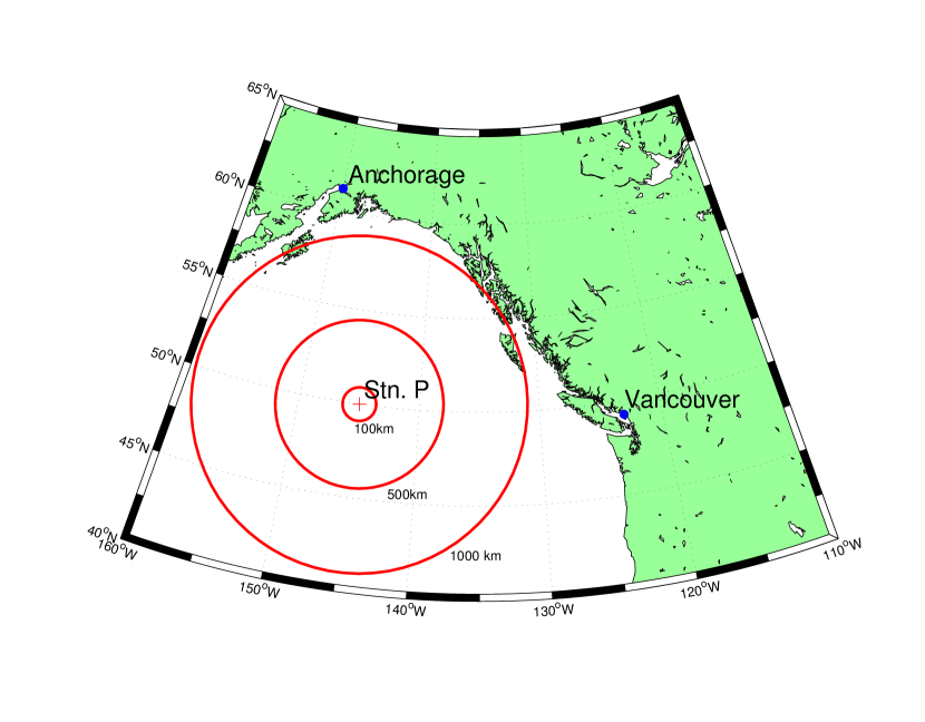
Figure 3: A map of the north-east Pacific Ocean displaying the location of Ocean Station Papa (Stn. P) with range circles at 100, 500 and 1000 km.

It has been noted that there are persistently high macro-nutrient concentrations in the mixed layer and the phytoplankton biomass is typically low. This phenomenon is observed throughout much of the open sub-arctic Pacific ocean. While the concentration of dissolved inorganic nitrogen (DIN) is lower in summer than in winter, it is rarely if ever depleted to levels that may cause nutrient limitation in primary producers (Harrison, 2002). There is no discernible seasonal cycle in chlorophyll-a. Previous modelling studies of Matear (1995), Denman and Pena (1999) and Denman (2003) discuss the likely controls on phytoplankton biomass and the seasonal variation in primary productivity and zooplankton biomass.

4.2 Learning from Observations: Twin Experiment with Climatological Forcing

Twin experiments in a setting like that of OSP have been conducted to compare samples from the posterior, $[{\bf W,\boldsymbol{\theta}}|{\bf{\bf{Y}}}]$, produced by Bayesian inference, with known “true” values of the state and parameters. The term “twin”, borrowed from the data-assimilation literature, refers to experiments where the model used for inference, and the model from which synthetic observations are generated, are the same. Model forcing and boundary conditions are taken from Matear (1995) and are climatological in nature; details are given in Appendix D.

4.2.1 Twin Experiment: Design

To generate the synthetic observations, we select a parameter set $\boldsymbol{\theta}^{*}$ (the “true” parameters) and take a single realisation of the stochastic model $\{\mathbf{W}^{*}_{t}:t=0,1,\ldots,T\}$ to produce the trajectory $\{\mathbf{X}^{*}_{t}:t=0,1,\ldots,T\}$ through state space (again referred to as the truth). We have chosen a set of “true” parameters in the twin experiment that are shifted away from the prior means (to provide a clearer test of the inference procedure), but that nevertheless yield state-variable trajectories qualitatively consistent with OSP observations (e.g., high-nutrient low-chlorophyll (HNLC) conditions). The (synthetic) observations $\mathbf{Y}$ are generated by:

$${\bf{Y}}_{t}={\bf{X}}^{*}_{t}\exp(\xi_{t});\;t=0,1,\ldots,T\,,$$ (24)

where $\xi_{t}$ are independent and identically distributed (IID) as the normal distribution $N(0,\sigma^{2}_{obs})$. The standard deviation, $\sigma_{obs}$, was $0.1$ for DIN observations and $0.2$ for observations of the remaining state variables. The log-normal error model was adopted because errors in the estimates of plankton density are typically better represented by log-normal multiplicative error than by additive normal error (Campbell, 1995), and the log-normal multiplicative-error model delivers synthetic observations that are non-negative. The observation errors are assumed to be independent over time, reflecting either analytical error or (more likely) uncorrelated small-scale variation in concentrations.

4.2.2 Twin Experiment: Results

We first generate an ensemble of model trajectories by sampling from the prior distribution for parameters and running the stochastic model forward through the period January 1971 - November 1974, without assimilating any observations. This so-called free-run process-model ensemble is precisely a sample from the prior distribution over the state (Figure 4, blue shading), which expresses the uncertainty in the state based only on the prior knowledge of the parameters gained from a meta-analysis of the literature. In spite of the large prior uncertainty in some of the process-model parameters, the median values of the (marginal) prior distributions over state variables show surprisingly similar qualitative behavior to the observed climatology at OSP (Figure 4, dark blue line). The median DIN values remain elevated, and median chlorophyll-a values remain low. However, the 95% contours of the prior ensemble include unrealistic behaviours not observed at OSP, involving near-complete depletion of DIN and intense phytoplankton blooms.

When the synthetic observations described in Section 4.2.1 are assimilated, using the methodology described in Section 3, the 95% credibility intervals for the posterior distribution of the state are very tightly constrained about the true trajectory (Figure 4, red shading), compared with the prior intervals and with the observations. Despite the 20% observation error, the dynamical BHM implemented through the PMCMC described in Appendix C, accurately tracks the true state (Figure 4, green line).

The case for N deserves additional explanation. The seasonally varying N concentration, prescribed below the mixed layer as a boundary condition, imposes a sharp upper limit to the predicted mixed-layer N concentrations. Provided grazing control keeps phytoplankton biomass and N utilization small, the predicted concentration is very close to this upper bound. In most prior trajectories, grazing control is effective, so the prior median is close to the upper limit. Some prior parameter combinations allow phytoplankton blooms and N depletion, resulting in the drawdown of N to near-zero levels seen in the prior lower 95th percentile for N. The truth is chosen to be OSP-like, and so produces N concentrations close to the upper bound. Since we add noise to the truth, a significant fraction of the observations lie above the upper bound.

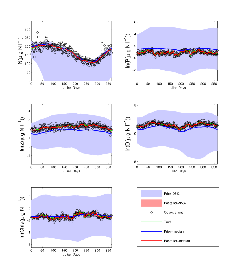
Figure 4: Twin experiment: a time series of the prior and posterior distributional properties of the state (X). Note that the posterior credibility intervals remain so close to the posterior median that they are difficult to distinguish. The figure legend is shown on the lower right.

The prior distributions over the parameters given in Table 1 of Appendix A.4 are the blue curves in Figure 5. These priors are discussed in Section 3.2 and are considered “global” in that they represent experimental results encompassing a wide range of species and domains. For some model parameters ($a_{Ch}$, $s_{D}$, $PDF$, $ZDF$, $\mu_{g^{max}}$, $\mu_{\lambda^{max}}$, $\mu_{Cl_{Z}}$, $\mu_{E_{Z}}$, $\mu_{r_{D}}$, and $\mu_{m_{Q}}$), the marginal posteriors in Figure 5 show evidence of learning in that the posterior mode has moved towards the truth and the posterior variances have contracted compared with the prior. However, for others, the inference procedure appears to extract little or no information from the data, and the marginal posteriors appear to merely recover the prior distributions. This is true for the parameters controlling light attenuation due to water ($K_{W}$), the fraction of zooplankton waste diverted to detritus ($f_{D}$), the parameters related to nitrogen uptake and nitrogen:carbon ratios ($a_{N}$ and $R_{N}$), and the maximum zooplankton ingestion rate ($I_{Z}$). In the case of $a_{N}$, the posterior variance is slightly reduced, but the posterior median remains centred at the prior mean.

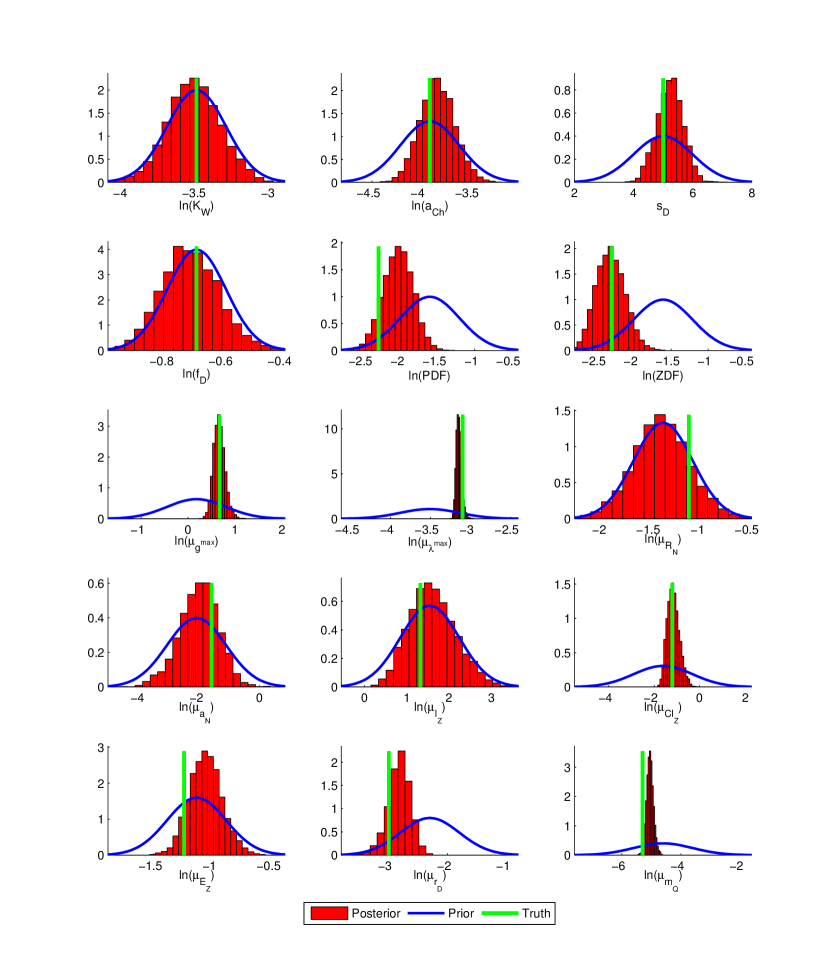
Figure 5: The prior (blue curve) and posteriors (red histogram) for each of the parameters. The true value is given by the vertical green line.

The inference procedure generates posterior distributions for time series of the autoregressive processes $\mathbf{B}(t)$, and could provide information about changes over time in the ecophysiological properties they represent. However, the results from this twin experiment are only mildly encouraging in this regard. In cases where the observations are uninformative about the parameters underlying the autoregressive processes, one can hardly expect to obtain information about the temporal variation in the processes themselves. Indeed, in those cases, the posteriors for the stochastic-process trajectories are the same as the priors. In two cases ($g^{max}$ and $Cl_{Z}$), the posterior median trajectories appear to track the truth, although with consistent bias in the case of $Cl_{Z}$ (Figure 6). But for these, and all other autoregressive processes, the 95% credibility interval for the posterior exceeds the amplitude of the temporal variation in the truth by some margin. The inference procedure does not allow us to conclude that there are significant changes in these processes over time.

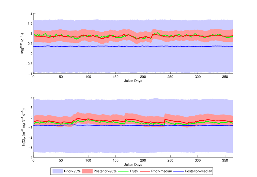
Figure 6: Twin experiment: a time series of the prior and posterior distributional properties of the autoregressive processes ($\mathbf{B}(t)$).

These results reflect the particular nature of the climatological forcing and system behavior at OSP. Given that concentrations of dissolved inorganic nitrogen at OSP remain well above levels expected to limit phytoplankton growth, it is unsurprising that parameters controlling nitrogen limitation of growth rates are poorly constrained. Similarly, phytoplankton biomass remains at levels well below those required to saturate zooplankton grazing, and zooplankton growth rates are controlled by the clearance rate $Cl_{Z}$, not by the maximum ingestion rate.

4.3 Learning from Observations: Ocean Station Papa Dataset

To demonstrate the application of the BHM approach to a real dataset, we have used a subsample of historical OSP data.

4.3.1 Ocean Station Papa - Data Model

Observations of nitrate (DIN) and chlorophyll-a taken between January 1971 and November 1974 are used. Observation errors are large and dominated by spatial sampling errors, because we neglect horizontal advection and assume a large model domain with high levels of within-domain variability. The presence of larger observation errors means that the data will be less informative. We draw on a number of studies below for estimates of the appropriate levels of spatial variability.

The spatial and temporal variability of Particulate Organic Carbon (POC) in this region has been investigated at a number of scales (Bishop et al., 1999). The spatial variability in the vertical and horizontal directions was calculated from the beam-attenuation coefficient obtained from a transmissometer.

• Small-scale horizontal variability (1-10km) of POC appears to be 5% to 10%, which is deemed negligible in comparison to the ocean scale and temporal variability.

• Large-scale horizontal variability (100-300km) of POC appears to range from 10% to 40%, however we attribute some of this variability to the passage of weather systems on time scales of 5 to 10 days.

• Ocean-basin-scale variability (800-2000km) exceeds both the large-scale and small-scale spatial variability, but this is due to the change from HNLC conditions in the deep ocean to a more typical temperate seasonal cycle on the continental shelf.

Bishop et al. (1999) also noted significant interannual variability that may be linked to El Niño events. Nitrate data collected along the Line P transect (a 1425 km long transect between the coast adjacent to the Juan de Fuca strait and Ocean Station Papa (e.g. Pena and Bograd, 2007)) from 1992 to 1997 display a similar pattern to the POC data. Again, it appears that on the scale of 100-300km around OSP, variability in total concentrations of nitrates and nitrites appears to be 10% to 30%, with inter-annual variability exceeding the large-scale spatial variability (Whitney and Freeland, 1999).

Taking all these sources of information into account, we have assigned a CV ($\sigma_{\text{obs}}$) of 0.5 to the observation error for both DIN and chlorophyll-a. This is a conservative (upper) estimate, representing an upper bound to spatial variation, and allowing for other non-spatial contributions, including analytical measurement error.

4.3.2 Ocean Station Papa - Results from Hindcast

A prior ensemble over the state was constructed in a similar manner to the twin experiment, using real forcing from January 1971 to November 1974. Model parameters were sampled from the prior distributions described earlier. As in the twin experiment in Section 4.2, a wide range of model behaviors was observed (Figures 7 and 8), ranging from near-complete depletion of DIN during summer, to year-round grazing control. As in the twin experiment, the median of the prior over the state based on 1971-1974 forcing qualitatively agreed with observed OSP behavior, in that DIN was never limiting, and there were no strong phytoplankton blooms as zooplankton grazing maintained relatively constant phytoplankton biomass (Matear, 1995; Denman and Pena, 1999; Denman, 2003).

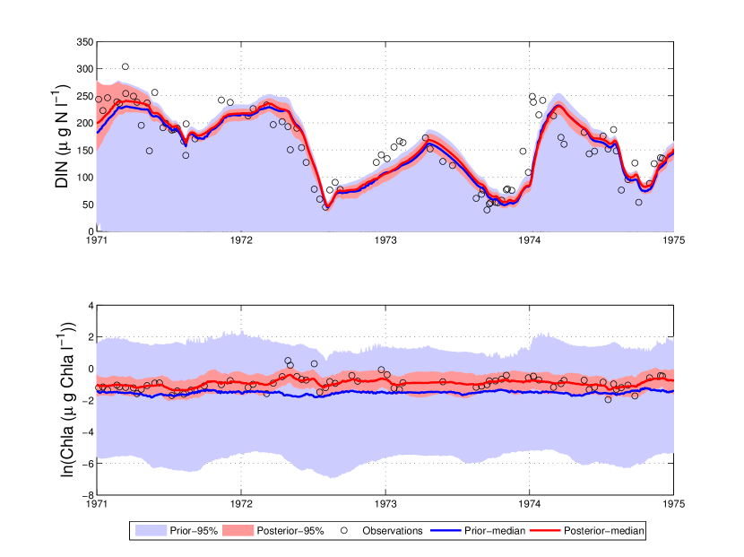
Figure 7: A time series of prior and posterior distributional properties of observed state variables, comparing observations (open black circles), prior (blue) and posterior (red).

When observations of chlorophyll-a and DIN are assimilated, the 95% credibility interval is dramatically reduced. Due to the relatively large observation error prescribed (see Section 3.3), the transient, low-magnitude increase in chlorophyll-a seen in the summer of 1972 is absorbed into the observation error and not tracked in the state. While the three individual observations of this anomalous bloom do not fall within the posterior 95% credibility interval, this cannot be interpreted immediately as lack of model fit. This is because the credibility interval depicted is over the latent chlorophyll-a state variable, not over the “noisier” observed chlorophyll-a; this distinction is important and is discussed by Cressie and Wikle (2011, Section 2.2.2). Although short-lived transient features are not tracked by the model, slow seasonal and intra-seasonal variations are well captured. The methods described in Section 2.3 not only condition the state on observations from previous times, as do filtering approaches, but also on future times. This is referred to as smoothing in the Bayesian filtering literature (Briers et al., 2010; Fearnhead et al., 2010). The advantage of such smoothing is evident in time periods where there are very few observations (e.g., mid-1973).

Through the process model, Bayesian methods allow inference on the unobserved state variables $P$, $Z$ and $D$; see Figure 8. Notice that there is a substantial reduction in the uncertainty expressed through the posterior compared with that expressed through the prior, even for unobserved state variables. For example, there is a strong seasonal cycle in the zooplankton biomass, which has been observed in a number of studies (Harrison, 2002). The peak in the zooplankton biomass occurs during mid summer, which coincides with a peak in primary production (not shown).

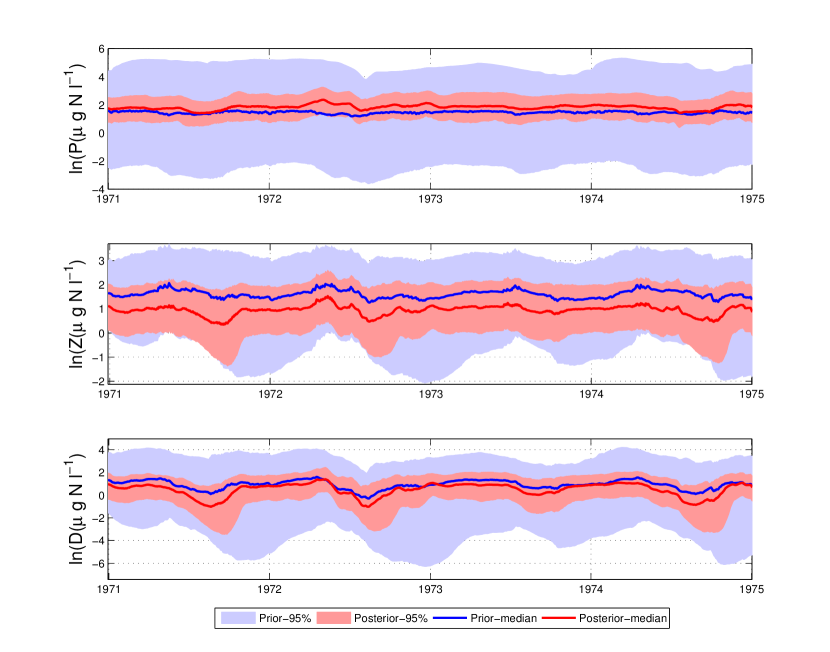
Figure 8: A time series of prior and posterior distributional properties of unobserved state variables comparing prior (blue) and posterior (red).

The marginal posteriors for model parameters shown in Figure 9 demonstrate that the sparse and limited OSP observations carry very little information about many of the parameters. This was not unexpected; previous studies have also experienced difficulty in using the OSP dataset to estimate parameters in deterministic models (Matear, 1995). The large observation variances used here, which compensate for effects of advection, reduce the effective information content of the data, but we believe this is realistic, given the model structure. The posterior marginals show evidence of learning for four parameters: $ZDF,g^{max},\mu_{Cl_{z}}$ and $\mu_{I_{z}}$.

Perhaps unsurprisingly, given the high noise levels and sparse observations, the OSP data do not allow us to derive useful information about temporal variation in the autoregressive processes $\mathbf{B}(t)$. Even for those parameters, $g^{max}$ and $Cl_{z}$, where the observations appear to inform the posteriors for the underlying parameters, the posteriors for the autoregressive trajectories show no significant variation over time (not shown).

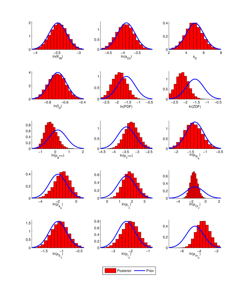
Figure 9: A comparison between the prior (blue curve) and the posterior (red histogram) for all parameters $\boldsymbol{\theta}_{\mathbf{X}}$ and $\boldsymbol{\theta}_{\mathbf{B}}$.

One advantage of the BHM framework is that we can use the sample generated from the joint posterior of the state and parameters, conditioned on past observations, to assess the uncertainty in model forecasts and scenarios. In this case, we have used the posterior conditional on observations from January 1971 to November 1974 to make a probabilistic forecast for 1975. We do this simply by propagating all posterior trajectories forward the additional year, using the boundary and forcing fields for that year. The results from this forecast ensemble (median and 95% credibility intervals) are shown in Figure 10. Agreement with the (non-assimilated) observations in the forecast period is very good.

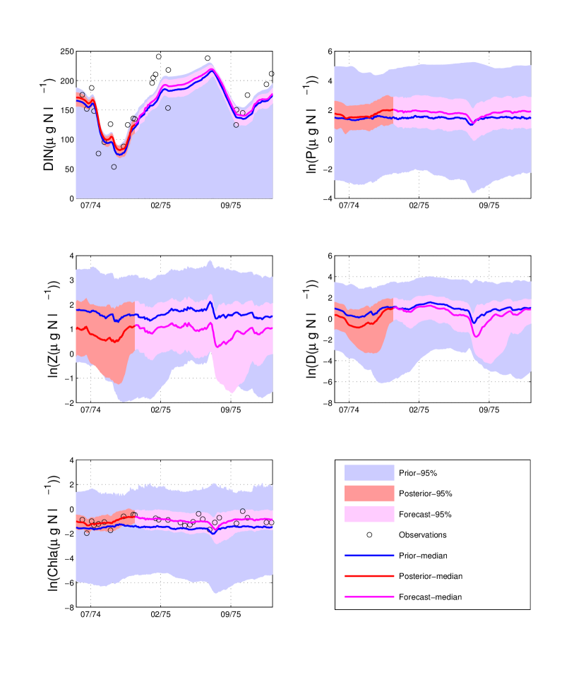
Figure 10: A forecast (magenta shading) for the model’s state variables for the period December 1974 - December 1975. The posterior and prior of the state are given by the red and blue shading, respectively. Observations are denoted by the open black circles; during the forecast period, the observations were not assimilated.

5 Discussion and Conclusions

A key consideration in building BHMs is the treatment of model error. In our study we used the fact that the aggregation of communities of species into single trophic levels or functional groups, and the replacement of well defined eco-physiological parameters for individual species by community-average parameters, is an important source of model error. Consequently, we have replaced the constant community parameters used in most biogeochemical models by stochastic autoregressive processes that vary slowly in time. This is in contrast to the common approach of simply adding white noise to the rate equations.

A potential drawback of this approach is that it increases the complexity and dimensionality of the model and the inference problem. We have augmented the four-dimensional primary state space $(N,P,Z,D)$ with nine additional state variables ($\mathbf{B}$). Instead of estimating nine constant parameters, we must estimate nine means and nine variances controlling the evolution of the stochastic processes $\mathbf{B}(t)$. We have mitigated this problem by using prior information to set the relative magnitudes of the variances of phytoplankton and zooplankton community parameters, and using stochastic factors related to community diversity to set the absolute magnitude. One advantage of the process model, as formulated, is that it allows a strong and direct connection to literature meta-data on the distributions of eco-physiological parameters across species. This allows us to set informative objective priors for most of the parameters, exploiting a key advantage of Bayesian approaches, and partially counterbalancing the increase in unknowns.

The inference procedure was designed to derive joint posteriors for system parameters and the (augmented) system state. Many examples of data assimilation in dynamical models concentrate on either state estimation or parameter estimation. Joint inference is particularly difficult in nonlinear models with sparse data, and it has typically required strong simplifying approximations, such as the replacement of nonlinear dynamics by approximating linear models. The underlying deterministic NPZD model is highly nonlinear, displaying two qualitatively different modes of behaviour or local stability domains, and the observed behaviour at OSP correspond to only one of these domains. The new particle MCMC techniques employed here are able to cope with this nonlinear, threshold behaviour, but are computationally expensive.

Given these challenges, the results of the OSP case study offer a number of grounds for encouragement. First, the stochastic process model allows the construction of priors over the model state, by drawing random samples from the prior distribution for model parameters and initial conditions, and running ensembles of model simulations. We can think of this prior ensemble as encapsulating our ability to predict system behaviour at OSP, given independent scientific knowledge about BGC processes, and local environmental forcing, but no other local knowledge. Encouragingly, the state median in these prior distributions bears a strong qualitative and even quantitative resemblance to OSP observations (Figures 4, 7), even though the priors were chosen to reflect the full range of species attributes reported in the literature. But the 95% credibility intervals for the prior distribution also include trajectories involving phytoplankton blooms and nitrate depletion, which are incompatible with observations at OSP.

Data assimilation into dynamical process models can serve a variety of different diagnostic and prognostic purposes (see e.g., Gregg, 2008; Luo et al., 2011). One class of diagnostic applications targets the hindcasting or nowcasting of system state, given limited observations. Despite sparse observations with large sampling errors on one state variable ($N$) and one diagnostic variable ($Chla$), the Bayesian inference procedure recovers quite tight posteriors for these observed variables (Figure 7). The Bayesian inference procedure is also able to transfer information from observed to unobserved state variables, reducing the uncertainty in the unobserved state variables ($P$, $Z$ and $D$) by about half (Figure 8).

A second class of diagnostic applications focuses on learning about, and interpretation of, model parameters. Here, the parameters describe the ecological characteristics of the plankton communities present at OSP. To the extent that these parameters have smaller variances a posteriori, we can conclude that the observations have provided information about the parameters and the communities they represent. The results for OSP are informative and cautionary. In the twin experiment, with observations on all state variables, the posteriors for some parameters are essentially identical to the priors, so provide no additional information (Figure 5). These results can be explained in terms of model dynamics. Since nutrients under OSP conditions are always saturating, and phytoplankton concentrations remain low, the parameters affecting phytoplankton growth at low nutrient concentrations, and zooplankton ingestion at high phytoplankton concentrations, have negligible effect on model predictions, and are not identifiable. This pattern of identifiability is an intrinsic characteristic of the environmental forcing and dynamics at OSP. In other ocean conditions, such as oligotrophic mixed layers where nutrient concentrations are always low and limiting, one would expect different sets of model parameters to be identifiable.

Using the limited set of historical observations available for OSP, the inference procedure is able to extract information about a few key parameters only (Figure 9). For the most part, these parameters directly control the key processes involved in zooplankton grazing control of phytoplankton. The posterior distributions for the parameters controlling the variance in model parameters (PDF and ZDF) are shifted towards lower values, compared with the priors. At the inferred lower levels of stochastic noise, trajectories are less likely to escape the local stability domain corresponding to grazing control.

The Bayesian inference procedure provides posterior distributions for the trajectories of the stochastic BGC processes, $\mathbf{B}(t)$. Reliable information on changes in these processes would be of particular interest to plankton ecologists. However, even in a twin experiment with daily data on all state variables, we were only able to obtain suggestive (but not confirmatory) information about temporal variation in two parameters. This limited success is understandable, given that we are effectively trying to extract information about changes in unobserved variables on relatively short time scales, when the evidence of these changes is available only indirectly through changes in the time derivatives of the observed state variables. Even modest levels of observation noise are sufficient to confound this attempt. We conclude that higher frequency observations, and /or lower observation noise, would be required to learn about temporal variation in these community properties from observations of state variables alone.

A twin experiment with similar forcing, sampling pattern and observation noise to the historical OSP observations yielded qualitatively equivalent results to those obtained using the real data. While not conclusive, this does suggest that the limited information about state and parameters obtained using the historical observations may be attributed to their sparseness and high observation noise, rather than an inconsistency with structural model assumptions.

It is common practice to distinguish short-term forecasts, in which uncertainty is dominated by the error in estimates of the current system state, from longer-term forecasts or projections, in which uncertainty may be dominated by errors in model structure, errors in parameter estimates, and the underlying stochastic process error. The methods used here allow us to move seamlessly from short-term to long-term forecasts. The forecast results are encouraging (Figure 10), especially given that the inference procedure and observations have provided information about a small subset only of model parameters. This limited information, combined with prior information on other parameters, is sufficient to produce a long-term forecast that agrees both qualitatively and quantitatively with observations.

Given the limited identifiability of both parameters and the related stochastic biogeochemical processes, one could reasonably ask whether the model is over-parameterised. This would be the case if we were building a model specifically for the purpose of explanation or prediction at OSP that ignored prior information on model structure and parameters. However, we are engaged in developing a generic model, based on well accepted principles and strong prior information. The model is applied at OSP, but we envisage the same model (or a similar model) being applied at many other locations, and in the long run used as a basis for basin-scale or global BGC models spanning many different environmental conditions. Under these circumstances, it would be inappropriate to eliminate processes from the model on the grounds that they are not important at OSP, or that they are not identifiable from a particular set of historical observations from OSP. We are interested rather in the question of what such a model allows us to infer and predict about OSP and other regions, given generic objective prior information and the limited available observations.

Models with many, poorly identified parameters can be subject to over-tuning and poor predictive performance, especially if parameter estimation procedures are heuristic, and/or are designed to produce a single “optimal” parameter set. The BHM framework and inference procedures used here provide protection against over-tuning. The posterior distribution yields samples from the full range of possible parameters and states, conditional on priors and observations, and it therefore provides a realistic picture of the effects of equifinality (Von Bertalanffy, 1969; Beven and Binley, 1992) on model hindcasts and predictions. The performance of the posterior for the long-term forecast for OSP (Figure10) supports this conclusion.

Emerging observing systems promise much richer data sets than in the past. New automated in situ and remote sensors can provide data for more variables with much higher temporal resolution and/or spatial coverage. The twin experiment with daily observations presented here provides a hint of what we might expect from such improved observing systems. Data assimilating models are increasingly being used to assess the information value of alternative observing system designs, as part of so-called Observing System Simulation Experiments (OSSEs; e.g., Masutani et al., 2010). The twin experiments presented were intended primarily as a check on the consistency and performance of the inference methods; an OSSE would require careful attention to observing system elements and costs, and the use of replicate experiments. We anticipate using the BHM framework to build OSSEs. Oceanographic field studies often include local in situ or ship-board experiments that effectively measure the instantaneous values of community ecophysiological properties. The model formulation proposed here offers the opportunity to integrate these measurements with standard observations of state variables (biomass) within a consistent and rigorous inference framework. We see this as an interesting direction for further research using both OSSEs and real observations.

We recognise that, in order to fully exploit the potential for OSSEs, and for hindcasting and forecasting more generally, it will be necessary to extend our approach from the 0-D box model considered here to spatially resolved models, including both 1-D vertical mixing models (e.g. Mattern et al., 2010) and 3-D circulation models (cf. Gregg, 2008). The adoption of spatially resolved models would avoid the ambiguity about spatial scales inherent in the box model and allow a more rigorous treatment of spatial sampling errors. We do not foresee major conceptual problems in extending the formulation to spatially resolved models, but Bayesian inference in these models will involve formidable computational challenges, and may require the development of effective approximate techniques.

We believe that the example presented here delivers at least in part on the promise described by Berliner (2003) and Cressie et al. (2009) of BHM as a self-consistent probabilistic framework that integrates statistical and mechanistic process models. The specific process model developed here shows promise as a basis for applications for many local and regional aquatic BGC applications. We hope that some of the methods developed here, including the use of stochastic processes for aggregate community properties, will find broader application.

Appendix A Process Model: Supplementary Material

A.1 A simple adaptive model of phytoplankton growth and composition in response to light, nutrient, and temperature.

The phytoplankton growth model used in this paper predicts changes in phytoplankton specific growth rate $g$ and composition (nitrogen:carbon chlorophyll-a:carbon ratios) in response to changes in incident irradiance $E$, temperature $T$, and dissolved inorganic nitrogen $N$. The formulation represents a compromise between realism and complexity. Consistent with the BHM framework, we have sought a formulation that explicitly connects the key observed quantity chlorophyll-a ($Chla$) to the state variable of phytoplankton biomass ($P$) using the common currency of nitrogen. By explicitly treating changes in nitrogen:carbon ratios as well, the formulation would also support observations of dissolved oxygen or dissolved inorganic carbon, although we do not treat those in this paper. At the same time, we have avoided introducing additional hidden state variables, and we have sought to minimize the number of new parameters.

This formulation draws on the adaptive phytoplankton growth model of Geider et al. (1998), who specified the carbon-specific phytoplankton growth rate, $g_{C}$, and the nitrogen-specific phytoplankton growth rate, $g_{N}$, as follows:

$$g_{C}=g^{m}_{C}.(1-\exp(-\alpha.\lambda.E/g^{m}_{C})),$$ (25)

$$g^{m}_{C}=g^{max}.Tc.(\chi-\chi^{min})/(\chi^{max}-\chi^{min}),$$ (26)

$$g_{N}=V^{m}.N/(K+N),$$ (27)

$$V^{m}=V^{max}.Tc.(\chi^{max}-\chi)/(\chi^{max}-\chi^{min}).$$ (28)

Here, the temperature correction factor $Tc$ is based on a “$Q_{10}$ factor” (see Eq. (10) in the main text), $\lambda$ is the chlorophyll-a:carbon ratio, $K$ is the half-saturation constant for phytoplankton growth on $N$, and $\alpha$ is the initial slope of the photosynthesis versus irradiance curve. In Geider et al. (1998)’s model, the light-saturated $C$-specific phytoplankton growth rate, $g^{m}_{C}$, and the nutrient-saturated phytoplankton nitrogen-specific growth rate, $V^{m}$, depend on the nitrogen:carbon ratio, $\chi$, in a way that ensures that the ratio lies between $\chi^{min}$ and $\chi^{max}$. We may think of this formulation as an extensive version of a cell quota model.

Geider et al. (1998) introduced a third expression for the phytoplankton $Chla$-specific growth rate, $g_{Chl}$, as a function of $g_{C}$, $g_{N}$, $\lambda$, $E$, and $\chi$. Here, we have avoided introducing new dynamic state variables for phytoplankton carbon and phytoplankton chlorophyll-a. Instead, we have sought a solution for $g_{N}$, $\lambda$ and $\chi$, as functions of $T$, $N$ and $E$, under conditions of balanced growth when $g_{C}=g_{N}=g_{Chla}$. It is not possible to derive an explicit expression for these solutions in the original model. However, it is possible to do so with the following key simplification.

Behrenfeld et al. (2005) argue that phytoplankton adjust their chlorophyll-a:carbon ratio, $\lambda$, so that it is proportional to $g^{m}_{C}$ under balanced growth. We assume that, at steady-state,

$$\lambda=\lambda^{max}.g^{m}_{C}/g^{max},$$ (29)

and substituting (29) into (25) gives

$$g_{C}=g^{m}_{C}.(1-\exp(-\alpha.\lambda^{max}.E/g^{max})).$$ (30)

We define $g^{*}_{E}$ as the maximum $C$-specific phytoplankton growth rate for given irradiance $E$ and temperature $T$. This is achieved at $\chi=\chi^{max}$ and is given by:

$$g^{*}_{E}=g^{max}.Tc.(1-\exp(-\alpha.\lambda^{max}.E/g^{max})).$$ (31)

We define $g^{*}_{N}$ as the maximum $N$-specific phytoplankton growth rate for given nutrient concentration $N$ and temperature $T$. This is achieved at $\chi=\chi^{min}$ and is given by:

$$g^{*}_{N}=V^{max}.Tc.N/(K+N).$$ (32)

Now, $g_{C}=g^{*}_{E}.(\chi-\chi^{min})/(\chi^{max}-\chi^{min})$, and $g_{N}=g^{*}_{N}.(\chi^{max}-\chi)/(\chi^{max}-\chi^{min})$.

Under balanced growth, the specific growth rate $g=g_{C}=g_{N}$, and solving for $\chi$ gives:

$$\chi=(g^{*}_{E}.\chi^{min}+g^{*}_{N}.\chi^{max})/(g^{*}_{E}+g^{*}_{N}).$$ (33)

Substituting (33) into $g_{C}=g^{*}_{E}.(\chi-\chi^{min})/(\chi^{max}-\chi^{min})$, and appealing to the equality $g=g_{C}=g_{N}$, yields:

$$g=g^{*}_{E}.g^{*}_{N}/(g^{*}_{E}+g^{*}_{N})$$ (34)

and, from, (29)

$$\lambda=\lambda^{max}.Tc.g^{*}_{N}/(g^{*}_{E}+g^{*}_{N}).$$ (35)

These expressions have a simple and logical interpretation. The rates $g^{*}_{E}$ and $g^{*}_{N}$ are the potential specific phytoplankton growth rates determined by light and nutrient separately, and we can think of them as measures of light and nutrient availability as perceived by the cell. The achieved growth rate $g$ is a compromise between the two. If one is much larger than the other, then the achieved growth rate is very close to the smaller rate. Note that simple non-adaptive models of phytoplankton growth often multiply a light-limitation and a nutrient-limitation term. It is well known that this underestimates growth rates. Our approach partly avoids the defect of multiplicative growth models. In (33), the nitrogen:carbon ratio approaches $\chi^{min}$ when light is much more available than nutrient ($g^{*}_{E}>>g^{*}_{N}$), and it approaches $\chi^{max}$ when $g^{*}_{N}>>g^{*}_{E}$, as one might expect. The chlorophyll-a:carbon ratio, $\lambda$, approaches $\lambda^{max}$ when light is limiting and nutrient is abundant ($g^{*}_{N}>>g^{*}_{E}$), and it approaches zero when nutrient is strongly limiting and light is saturating.

It is possible to treat $g_{N}$ as an $N$-specific uptake rate, and for the maximum specific uptake rate of nitrogen ($V^{max}$) to be substantially larger than the maximum $C$-specific growth rate ($g^{max}$). This would allow rapid uptake of nitrogen in a dynamic quota model. However, given that we are considering only balanced growth here, we treat $g_{N}$ as a specific growth rate and assume $V^{max}=g^{max}$. We must then interpret $K$ as a half-saturation constant for growth rather than uptake:

$$K=\frac{g^{max}.T_{C}}{a_{N}}.$$ (36)

With this simplification (substitute (36) into the $N/(K+N)$ term of (32)), we can write:

$$h_{N}=N/((g^{max}.Tc/a_{N})+N),$$ (37)

and from (31) we set

$$h_{E}=1-\exp(-\alpha.\lambda^{max}.E/g^{max}).$$ (38)

As before, under the assumption of balanced growth ($g=g_{C}=g_{N}$), we obtain

$$g=Tc.g^{max}.h_{E}.h_{N}/(h_{E}+h_{N}),$$ (39)

and

$$\chi=(h_{E}.\chi^{min}+h_{N}.\chi^{max})/(h_{E}+h_{N}).$$ (40)

If we set $R_{N}$ = $\chi^{min}/\chi^{max}$, then

$$\chi=\chi^{max}.(h_{E}.R_{N}+h_{N})/(h_{E}+h_{N}),$$ (41)

and

$$\lambda=\lambda^{max}.Tc.h_{N}/(h_{E}+h_{N}).$$ (42)

The phytoplankton chlorophyll-a:nitrogen ratio equals $\lambda/\chi$, and it is given by:

$$Chla:N=(\lambda^{max}.Tc/\chi^{max}).h_{N}/(h_{E}.R_{N}+h_{N}).$$ (43)

A.2 The transport operator

In this section we describe the transport operator, ${\bf T}({\bf c},{\bf x},t)$, used in equation (5) in the main text. The specific form applied to each of the state variables differs based on the characteristics of the specific state variable being operated on.

The change in mixed layer depth ($MLD$) is given by:

$$\psi(t)=\frac{d(MLD)}{dt},$$ (44)

and we define

$$\psi^{+}(t)\equiv max\left\{\psi(t),0\right\}.$$ (45)

This form of exchange across the mixed-layer has been adopted from Evans and Parslow (1985). Therefore the state equations, including the effects of changes in the mixed layer, can be written as:

$$\frac{dP}{dt}=g\cdot P-gr\cdot Z+\frac{\kappa+\psi^{+}(t)}{MLD}\cdot(BCP-P),$$ (46)

$$\frac{dZ}{dt}=E_{Z}\cdot gr\cdot Z-m\cdot Z+\frac{\psi(t)}{MLD}\cdot(BCZ-Z),$$ (47)

$$\frac{dD}{dt}=(1-E_{Z})\cdot f_{D}\cdot gr\cdot Z+m\cdot Z-r\cdot D-S_{D}\cdot D/MLD+\frac{\kappa+\psi^{+}(t)}{MLD}\cdot(BCD-D),$$ (48)

$$\frac{dN}{dt}=-g\cdot P+(1-E_{Z})\cdot(1-f_{D})\cdot gr\cdot Z+r\cdot D+\frac{\kappa+\psi^{+}(t)}{MLD}\cdot(BCN-N),$$ (49)

where $\kappa$ is the background mixing, $S_{D}$ is the detrital sinking rate (a parameter subject to inference), and $BCP$, $BCZ$, $BCD$ and $BCN$ are the boundary conditions for $P,Z,D$ and $N$, respectively. With the exception of $BCN$ all other state variable boundary conditions are set to 0. It is assumed that as the mixed layer shoals, $P,D$ and $N$ are lost from the mixed layer, whereas $Z$ is assumed to be retained in the mixed layer. As the mixed layer deepens, $P,Z$ and $D$ concentrations will be diluted, whereas $N$ will be added in an amount proportional to the prescribed boundary condition $BCN$. The variables $\kappa,\psi,MLD$ and $BCN$ are considered to be exogenous forcing and are prescribed.

A.3 The light model

$$E=E_{0}.(1-\exp(-Kz))/Kz,$$ (50)

where $E_{0}$ is the mean daily photosynthetically available radiation (PAR) just below the air-sea interface, and $Kz$ is given by:

$$Kz=(K_{W}+a_{Ch}\cdot Chla)\cdot MLD.$$ (51)

In (51), $K_{W}$ is attenuation due to the seawater, $a_{Ch}$ is attenuation due to $Chla$ and $MLD$ is the mixed layer depth.

A.4 The parameter (prior) model

Where possible, the priors for the process-model parameters have been based on information in the literature. The parameters can be divided into three classes.

For some physiological parameters, there are existing meta-analyses in the literature that provide estimates of parameter means and variances. Previous studies of phytoplankton by Tang (1995) and Montagnes et al. (1994), and of zooplankton by Hansen et al. (1997), have derived allometric relationships (log-log regressions) for phytoplankton and zooplankton parameters $g^{max}$, $\lambda^{max}$, $E_{Z}$, $Cl_{Z}$ and $I_{Z}$ as a function of individual size. From these data sets, we have derived prior means and coefficients of variation (Table 1), assuming that the phytoplankton community at OSP is dominated by small cells (mean cell volume 100 $\mu$m³), and grazing is dominated by microzooplankton (mean individual volume $10^{5}\mu$m³). We have used normal prior distributions for those parameters having small coefficient of variation, and log-normal prior distributions for the rest.

For some parameters, we can draw on a range of quoted values in the literature that are sufficient to provide crude estimates of prior mean and variance. Historical observations of the light attenuation due to water, $K_{W}$, and the specific absorption coefficient for chlorophyll-a, $a_{Ch}$, were taken from Kirk (1994). The maximum quantum yield is assumed constant at 0.1 mol $C$ mol photons^-1, or 1200 mg $C$ mol photons^-1. Estimates of the affinity of phytoplankton for dissolved inorganic nitrogen, $a_{N}$, are based on data in Hein et al. (1995) and on theoretical calculations of the diffusion limit to uptake.

Other parameters can be regarded as semi-empirical, representing ecosystem properties and processes that are only crudely represented in the model. We do not model zooplankton respiration explicitly, and we assume that approximately half of the ingested nitrogen that does not appear as an increase in biomass is released as unassimilated fecal pellets, and half is lost through respiration and excretion of dissolved inorganic nitrogen (cf. Parsons and Takahashi, 1973), so $f_{D}$ is given a prior mean of 0.5 and a small CV of 0.1 (Table 1). Because zooplankton grazing is assumed to be dominated by micro-zooplankton, we have assigned the detrital sinking rate $S_{D}$ a relatively small prior mean of 5 m d^-1, with a large CV of 1.0.

Detrital organic matter comprises diverse organic compounds that vary widely in their susceptibility to bacterial attack and remineralization. In the model, very labile organic nitrogen compounds such as amino acids, which may be utilized and remineralized on time scales of hours, are treated implicitly as part of the fraction $(1-E_{Z}).(1-f_{D})$ of ingestion that is released directly as dissolved inorganic nitrogen. A mean remineralization rate of 0.1 d^-1 is applied to the remaining detritus, with a relatively large CV of 0.5. The quadratic mortality rate for zooplankton, $m_{Q}$, is an empirical ecosystem parameter, representing the density-dependent predation on micro-zooplankton. It has been assigned a mean value of 0.01 d^-1 (mg $N$ m^-3)^-1, corresponding to a mortality rate of 0.1 d^-1 at typical micro-zooplankton biomass levels of 10 mg $N$ m^-3. Because we have little prior information to constrain $m_{Q}$, we have assigned it a large CV of 1.0.

The scale factors $PDF$ and $ZDF$ have been assigned a prior mean of 0.2. This is a relatively low value, and it corresponds to a diverse community in which the community mean properties show substantially less variation than those of individual species (see Appendix B). The prior variance is set to 0.4, so the prior distribution allows higher values of $PDF$ and $ZDF$, and also less diverse communities.

Table 1: The priors on parameters used in the stochastic NPZD model are all log-normal, with mean ($\mu$) and standard deviation ($\sigma$) on the log-scale, except for $S_{D}$ which is Gaussian.

Parameter	Description	Mean($\mu$)	SD ($\sigma$)
$K_{W}$	Light Attenuation: Water	0.03 m-1	0.2
$a_{Ch}$	Light Attenuation: Chla	0.04 m2 mg Chla-1	0.3
$S_{D}$	Detrital Sinking Rate	5 m d-1	1.0
$f_{D}$	Fraction of grazing to detritus	0.5	0.1
$PDF$	Phytoplankton Diversity Factor	0.15	0.4
$ZDF$	Zooplankton Diversity Factor	0.15	0.4
$\mu_{g^{max}}$	Maximum Carbon Specific Growth Rate	1.2 d-1	0.63
$\mu_{R_{N}}$	Ratio between $\chi^{min}$ and $\chi^{max}$	0.25	0.3
$\mu_{\lambda^{max}}$	Maximum $Chla$ to $C$ratio	0.03	0.37
$\mu_{a_{N}}$	Phytoplankton affinity for $N$	0.3 d-1 mg $N^{-1}$ m3	1
$\mu_{I_{Z}}$	Maximum Zooplankton ingestion rate	4.7 d-1	0.7
$\mu_{Cl_{Z}}$	Maximum Zooplankton clearance rate	0.2 m3 mg $N^{-1}$ d-1	1.3
$\mu_{E_{Z}}$	Zooplankton growth efficiency	0.32	0.25
$\mu_{m_{Q}}$	Zooplankton quadratic mortality rate	0.01 d-1 mg $N^{-1}$ m3	1
$\mu_{r_{D}}$	Detrital remineralization rate	0.1 d-1	0.5

Appendix B Autoregressive Process with Log-Normal Innovations

Suppose that a time series $\{B(t)\}$ evolves according to an AR(1) process with an intrinsic time-scale of $\tau$. Then, from equation (20) in the main text,

$$B(t+1)=B(t)(1-1/\tau)+\zeta_{B}(t)/\tau.$$ (52)

The innovation sequence $\{\zeta_{B}(t)\}$ is independent of $\{B(t)\}$ and is assumed to follow a log-normal distribution, so that $Z=\log(\zeta_{B}(t))\sim N(\mu_{z},\sigma_{z}^{2})$. The moments of the log-normal distribution are immediately available from those of the normal distribution since $E[\zeta_{B}(t)^{s}]=E[\exp(sZ)]$, the moment generating function of the underlying normal distribution. We find then that

$$E(\zeta_{B}(t)^{s})=\exp(s\mu_{z}+s^{2}\sigma_{z}^{2}/2),\quad s\geq 0.$$ (53)

Hence the mean and variance of $\{\zeta_{B}(t)\}$ follow directly as

$$\mu_{\zeta} = \exp(\mu_{z}+\sigma_{z}^{2}/2),$$

$$\sigma^{2}_{\zeta} = \exp(2\mu_{z})(\exp(2\sigma_{z}^{2})-\exp(\sigma_{z}^{2})).$$ (54)

The coefficient of variation, $CV(\zeta_{B})=\sigma_{\zeta}/\mu_{\zeta}$, is given by

$$CV(\zeta_{B})=(\exp(\sigma_{z}^{2})-1)^{1/2},$$ (55)

and so it does not depend on the mean.

Assuming second-order stationarity of $\{B(t)\}$ requires that $|1-1/\tau|<1$, so $\tau>1/2$. Taking expectations on both sides of equation (52), we find (using an obvious notation):

$$\mu_{B}=\mu_{B}(1-1/\tau)+\mu_{\zeta}/\tau,$$ (56)

so

$$\mu_{B}=\mu_{\zeta}=\exp\left(\mu_{z}+\sigma_{z}^{2}/2\right).$$ (57)

Next, calculating the variance of both sides using the independence assumption above, we obtain again using an obvious notation):

$$\sigma^{2}_{B} = (1-1/\tau)^{2}\sigma^{2}_{B}+\sigma^{2}_{\zeta}/\tau^{2}$$ (58)

$$= (2\tau-1)^{-1/2}\sigma^{2}_{\zeta}.$$

Since $\mu_{B}=\mu_{\zeta}$,

$$CV(B)^{2} = CV(\zeta_{B})^{2}/(2\tau-1)$$ (59)

$$= \left(\exp(\sigma_{z}^{2})-1\right)/(2\tau-1).$$

We may apply this result as follows. Suppose a community is made up of $n$ species, each with biomass fractions $\{p_{i}:i=1,\dots,n;\sum p_{i}=1\}$, and suppose further that the species-specific growth rate parameters $\boldsymbol{\phi}_{i}$ are log-normally distributed, where $log(\boldsymbol{\phi}_{i})$ has mean $\mu_{l\phi}$ and variance $\sigma_{l\phi}^{2}$. We are interested in the biomass-weighted community value, $\Phi\equiv\sum{p_{i}}{\boldsymbol{\phi}_{i}}$. Hence,

$$E(\Phi) = \sum p_{i}E(\boldsymbol{\phi}_{i})$$ (60)

$$= \exp(\mu_{l\phi}+\sigma_{l\phi}^{2}/2).$$

Further,

$$var(\Phi)=\sum{p_{i}}^{2}var(\boldsymbol{\phi}_{i})=\sum{p_{i}}^{2}\exp(2\mu_{l\phi})(\exp(2\sigma_{l\phi}^{2})-\exp(\sigma_{l\phi}^{2})).$$ (61)

Thus,

$$CV(\Phi)^{2}=\sum{p_{i}}^{2}(\exp(\sigma_{l\phi}^{2})-1).$$ (62)

In our case, we want to choose $\mu_{\zeta}$ and $\sigma_{\zeta}$ so that $E(B)=E(\Phi)$ and $CV(B)^{2}=CV(\Phi)^{2}$. Using (57), (59), (60) and (62), we have

$$exp(\mu_{\zeta}+\sigma_{\zeta}^{2}/2) = \exp(\mu_{l\phi}+\sigma^{2}_{l\phi}/2),$$ (63)

$$(\exp(\sigma_{\zeta}^{2})-1)/(2\tau-1) = \sum{p_{i}}^{2}.(\exp(\sigma_{l\phi}^{2})-1).$$ (64)

Finally,

$$\mu_{z} = \mu_{l\phi}+\sigma_{l\phi}^{2}/2-\sigma_{z}^{2}/2,$$ (65)

$$\sigma_{z}^{2} = \log\left(1+(2\tau-1)\sum{p_{i}}^{2}(\exp(\sigma_{l\phi}^{2})-1)\right).$$ (66)

For those eco-physiological parameters modelled here as a stochastic autoregressive process $\{B(t)\}$, we derive prior estimates of $\mu_{l\phi}$ and $\sigma_{l\phi}$ from the literature. We treat the quantities $\sum p_{i}^{2}$ as constants. For the phytoplankton community, $\sum p_{i}^{2}\equiv PDF^{2}$, and for the zooplankton community $\sum p_{i}^{2}\equiv ZDF^{2}$. The diversity factors $PDF$ and $ZDF$ (recalling that these scale the prescribed $\sigma_{l\phi}$ values) and $\mu_{l\phi}$ are parameters subject to inference, and they are given prior distributions (see Appendix A.4).

Appendix C Particle Markov Chain Monte Carlo Sampling

For brevity, we use the notation ${\bf W}_{i:j}$ (where $i\leq j$) to denote the sequence $({\bf W}_{i},\ldots,{\bf W}_{j})$, and likewise for ${\bf Y}_{i:j}$. We may write the posterior distribution as

$$[{\bf W}_{1:T},\boldsymbol{\theta}_{\bf W},\boldsymbol{\theta}_{\bf{Y}}|{\bf Y}_{1:T}] = [\mathbf{W}_{1:T}|\boldsymbol{\theta}_{\bf W},\boldsymbol{\theta}_{\bf Y},\mathbf{Y}_{1:T}][\boldsymbol{\theta}_{\bf W},\boldsymbol{\theta}_{\bf Y}|\mathbf{Y}_{1:T}].$$ (67)

The first factor of Equation (67) may be computed using a particle filter (Gordon et al., 1993; Doucet et al., 2001), with parameters fixed according to a draw from the second factor, considered below. At time $t$, let $[\mathbf{W}_{1:t}|\boldsymbol{\theta}_{\bf W},\boldsymbol{\theta}_{\bf Y},\mathbf{Y}_{1:t}]$ be represented by a set of $N$ samples (particles) $\mathbf{w}^{i}_{1:t}$ with associated weights $\alpha^{i}_{t}$, for $i=1,\ldots,N$. Given $\{(\mathbf{w}^{i}_{1:t-1},\alpha_{t-1}^{i})\}$, we may recursively obtain $\{(\mathbf{w}^{i}_{1:t},\alpha_{t}^{i})\}$ by setting, for $i=1,\ldots,N$,

$$\mathbf{w}^{i}_{t} \sim [\mathbf{W}_{t}|\mathbf{W}_{t-1}=\mathbf{w}^{i}_{t-1},\boldsymbol{\theta}_{\bf W}]$$ (68)

$$\alpha^{i}_{t} = \alpha^{i}_{t-1}\cdot[\mathbf{Y}_{t}|\mathbf{W}_{t}=\mathbf{w}^{i}_{t},\boldsymbol{\theta}_{\bf Y}].$$ (69)

The procedure is initialised with $\mathbf{w}_{0}^{i}\sim[\mathbf{W}_{0}]$ and $\alpha_{0}^{i}=1$, for $i=1,\ldots,N$. After several iterations, the sample tends to degenerate to a situation where only a single particle has significant weight. For this reason, resampling is typically performed after each step, redrawing particles with probability proportional to weights, and resetting all weights to be identically one. This has the effect of eliminating particles of low weight and replicating particles of high weight (Gordon et al., 1993; Kitagawa, 1996).

Note that, by time $T$, the procedure has produced weighted samples of the target factor $[\mathbf{W}_{1:T}|\boldsymbol{\theta}_{\bf W},\boldsymbol{\theta}_{\bf Y},\mathbf{Y}_{1:T}]$ of Equation (67). Sampling-importance-resampling (SIR) may be used to obtain a single sample from among these, making a single multinomial draw from the set $\{\mathbf{w}^{i}_{1:T}\}$ with assigned probabilities $\{\alpha_{T}^{i}/\sum_{j=1}^{N}\alpha_{T}^{j}\}$.

Turning to the second factor of Equation (67), note that

$$[\boldsymbol{\theta}_{\bf W},\boldsymbol{\theta}_{\bf Y}|\mathbf{Y}_{1:T}] \propto [\mathbf{Y}_{1:T}|\boldsymbol{\theta}_{\bf W},\boldsymbol{\theta}_{\bf Y}][\boldsymbol{\theta}_{\bf W},\boldsymbol{\theta}_{\bf Y}],$$ (70)

and that a particle filter may again be used to compute the likelihood term:

$$[\mathbf{Y}_{1:T}|\boldsymbol{\theta}_{\bf W},\boldsymbol{\theta}_{\bf Y}] = [\mathbf{Y}_{1}|\boldsymbol{\theta}_{\bf W},\boldsymbol{\theta}_{\bf Y}]\prod_{t=2}^{T}[\mathbf{Y}_{t}|\mathbf{Y}_{1:t-1},\boldsymbol{\theta}_{\bf W},\boldsymbol{\theta}_{\bf Y}]$$ (72)

$$= \int_{-\infty}^{+\infty}[\mathbf{Y}_{1}|\mathbf{W}_{1},\boldsymbol{\theta}_{\bf Y}][\mathbf{W}_{1}]d\mathbf{W}_{1}\times$$

$$\prod_{t=2}^{T}\int_{-\infty}^{+\infty}[\mathbf{Y}_{t}|\mathbf{W}_{t},\boldsymbol{\theta}_{\bf Y}][\mathbf{W}_{t}|\mathbf{Y}_{1:t-1},\boldsymbol{\theta}_{\bf W},\boldsymbol{\theta}_{\bf Y}]d\mathbf{W}_{t}$$

$$\approx \prod_{t=1}^{T}\frac{1}{N}\sum_{i=1}^{N}\alpha_{t}^{i},$$ (73)

where we have assumed in arriving at the last line that resampling is performed at each recursion of the particle filter. See Andrieu et al. (2010) for details.

The computation of this likelihood facilitates a Metropolis-Hastings (Metropolis et al., 1953; Hastings, 1970) sampling of $[\boldsymbol{\theta}_{\bf W},\boldsymbol{\theta}_{\bf Y}|\mathbf{Y}_{1:T}]$. For each parameter sample accepted, a state sample is drawn from the same particle filter used to obtain a likelihood estimate, resulting in a full sample of the posterior distribution given by Equation (67).

Finally, we require a suitable proposal distribution for the Metropolis-Hastings sampler. In this work, we use the approximate (log-)normal posterior furnished by a joint unscented Kalman filter (Julier and Uhlmann, 1997; Wan and van der Merwe, 2000) performing online process and parameter inference. After some number of steps, this is discarded in favour of a (log-)normal proposal adapted from the history of posterior samples (Haario et al., 2001).

Appendix D Case Study: Supplementary Material

D.1 Forcing Data

The forcing data used for the climatological twin-experiment and case-study was derived from that used in the study outlined in Matear (1995). The exogenous forcing that was applied is given in Figure 11. The forcing used for the 1971-1975 OSP experiment using the historical observations was again derived from the dataset used by Matear (1995) and is contained in Figure 12. The time series of Mixed Layer Depth (MLD) is used in equation (5) in the main text to form the transport operator and is discussed in Appendix A.2. Furthermore, the daily change in MLD (44) is used to parameterise the exchange across the base of the mixed layer. The sub-Mixed Layer DIN is the boundary condition (BCN) referred to in Appendix A.2. The Mixed Layer Temperature is used in the temperature correction term (equation (10) in the main text) for many of the rate processes given in Section 3.1 in the main text and Appendix A.1, while the photosynthetic available radiation (PAR) immediately below the surface is used to drive the photosynthesis in the phytoplankton growth model (Appendix A.1).

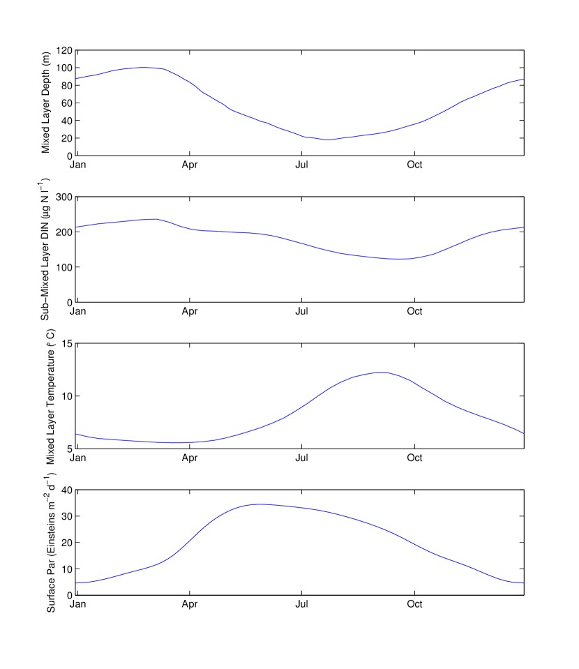
Figure 11: The climatological forcing obtained from Matear (1995) used in the twin experiment.

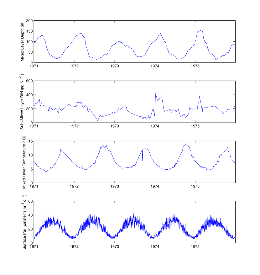
Figure 12: The forcing used in the Ocean Station Papa case study.

References

- Allen et al. (2007) Allen, J. I., J. T. Holt, J. Blackford, and R. Proctor. 2007. Error quantification of a high-resolution coupled hydrodynamic-ecosystem coastal-ocean model: Part 2. Chlorophyll-a, nutrients and SPM. Journal of Marine Systems 68:381–404.
- Andrieu et al. (2010) Andrieu, C., A. Doucet, and R. Holenstein. 2010. Particle Markov chain Monte Carlo methods. Journal of the Royal Statistical Society, Series B 72:269–302.
- Arhonditsis et al. (2008) Arhonditsis, G. B., G. Perhar, W. Zhang, E. Massos, M. Shi, and A. Das. 2008. Addressing equifinality and uncertainty in eutrophication models. Water Resources Research 44:W01420.
- Arhonditsis et al. (2007) Arhonditsis, G. B., S. S. Qian, C. A. Stow, E. Lamon, and K. H. Reckhow. 2007. Eutrophication risk assessment using Bayesian calibration of process-based models: Application to a mesotrophic lake. Ecological Modelling 208:215–229.
- Baker et al. (2006) Baker, D. F., S. C. Doney, and D. S. Schimel. 2006. Variational data assimilation for atmospheric CO2. Tellus, Series B 58:359–365.
- Barber and Gelfand (2007) Barber, J. J., and A. E. Gelfand. 2007. Hierarchical spatial modeling for estimation of population size. Environmental and Ecological Statistics 14:193–205.
- Behrenfeld et al. (2005) Behrenfeld, M., E. Boss, D. Siegel, and D. Shea. 2005. Carbon-based ocean productivity and phytoplankton physiology from space. Global Biogeochemical Cycles 19:GB1006.
- Berliner (2003) Berliner, L. M. 2003. Physical-statistical modeling in geophysics. Journal of Geophysical Research 108:doi:10.1029/2002JD002865.
- Berliner et al. (2000) Berliner, L. M., C. K. Wikle, and N. Cressie. 2000. Long-lead prediction of Pacific SSTs via Bayesian dynamic modeling. Journal of Climate 13:3953–3968.
- Beven and Binley (1992) Beven, K., and A. Binley. 1992. The future of distributed models: model calibration and uncertainty prediction. Hydrological Processes 6:279–298.
- Bishop et al. (1999) Bishop, J., S. Calvert, and M. Soon. 1999. Spatial and temporal variability of POC in the northeast Subarctic Pacific. Deep-Sea Research Part II-Topical Studies In Oceanography 46:2699–2733.
- Briers et al. (2010) Briers, M., A. Doucet, and S. Maskell. 2010. Smoothing algorithms for state-space models. Annals of the Institute of Statistical Mathematics 62:61–89.
- Calder et al. (2003) Calder, C. A., M. Lavine, P. Mueller, and J. S. Clark. 2003. Incorporating multiple sources of stochasticity in population dynamic models. Ecology 84:1395–1402.
- Campbell (1995) Campbell, J. W. 1995. The lognormal-distribution as a model for biooptical variability in the sea. Journal of Geophysical Research-Oceans 100:13237–13254.
- Clark and Bjornstaad (2004) Clark, J. S., and O. N. Bjornstaad. 2004. Population time series - Process variability, observation errors, missing values, lags, and hidden states. Ecology 85:3140–3150.
- Clark and Gelfand (2006) Clark, J. S., and A. E. Gelfand. 2006. A future for models and data in ecology. Trends in Ecology and Evolution 21:375–380.
- Cressie et al. (2009) Cressie, N., C. A. Calder, J. S. Clark, J. M. Ver Hoef, and C. K. Wikle. 2009. Accounting for uncertainty in ecological analysis: The strengths and limitations of hierarchical statistical modeling (with discussion). Ecological Applications 19:553–570.
- Cressie and Wikle (2011) Cressie, N., and C. K. Wikle. 2011. Statistics for Spatio-Temporal Data. Wiley, Hoboken, NJ.
- Denman (2003) Denman, K. 2003. Modelling planktonic ecosystems: parameterizing complexity. Progress In Oceanography 57:429–452.
- Denman and Pena (1999) Denman, K., and M. Pena. 1999. A coupled 1-D biological/physical model of the Northeast SubArctic Pacific Ocean with iron limitation. Deep-Sea Research Part II-Topical Studies In Oceanography 46:2877–2908.
- Doucet et al. (2001) Doucet, A., N. de Freitas, and N. Gordon, editors. 2001. Sequential Monte Carlo Methods in Practice. Springer, New York, NY.
- Dowd (2006) Dowd, M. 2006. A sequential Monte Carlo approach for marine ecological prediction. Environmetrics 17:435–455.
- Dowd (2007) Dowd, M. 2007. Bayesian statistical data assimilation for ecosystem models using Markov Chain Monte Carlo. Journal of Marine Systems 68:439–456.
- Dowd (2011) Dowd, M. 2011. Estimating parameters for a stochastic dynamic marine ecological system. Environmetrics 22:501–515.
- Dowd and Meyer (2003) Dowd, M., and R. Meyer. 2003. A Bayesian approach to the ecosystem inverse problem. Ecological Modeling 168:39–55.
- Evans and Parslow (1985) Evans, G. T., and J. S. Parslow. 1985. A model of annual plankton cycles. Biological Oceanography 3:327–347.
- Fearnhead et al. (2010) Fearnhead, P., D. Wyncoll, and J. Tawn. 2010. A sequential smoothing algorithm with linear computational cost. Biometrika 97:447–464.
- Geider et al. (1998) Geider, R., H. MacIntyre, and T. Kana. 1998. A dynamic regulatory model of phytoplanktonic acclimation to light, nutrients, and temperature. Limnology and Oceanography 43:679–694.
- Gordon et al. (1993) Gordon, N., D. Salmond, and A. Smith. 1993. Novel approach to nonlinear/non-Gaussian Bayesian state estimation. IEEE Proceedings-F 140:107–113.
- Gregg (2008) Gregg, W. W. 2008. Assimilation of SeaWiFS ocean cholophyll data Into a three-dimensional global ocean model. Journal of Marine Systems 69:205–225.
- Haario et al. (2001) Haario, H., E. Saksman, and J. Tamminen. 2001. An adaptive Metropolis algorithm. Bernoulli 7:223–242.
- Hansen et al. (1997) Hansen, P., P. Bjornsen, and B. Hansen. 1997. Zooplankton grazing and growth: Scaling within the 2-2,000-mu m body size range. Limnology and Oceanography 42:687–704.
- Harrison (2002) Harrison, P. 2002. Station Papa time series: Insights into ecosystem dynamics. Journal of Oceanography 58:259–264.
- Hastings (1970) Hastings, W. 1970. Monte Carlo sampling methods using Markov chains and their applications. Biometrika 57:97–109.
- Hein et al. (1995) Hein, M., M. Pedersen, and K. Sandjensen. 1995. Size-dependent nitrogen uptake in micro- and macroalgae. Marine Ecology-Progress Series 118:247–253.
- Holling (1965) Holling, C. S. 1965. The functional response of predators to prey density and its role in mimicry and population regulation. Memoirs of the Entomology Society Of Canada 45:60.
- Hood et al. (2006) Hood, R. R., E. A. Laws, R. A. Armstrong, N. R. Bates, C. W. Brown, C. A. Carlson, F. Chai, S. C. Doney, P. G. Falkowski, R. A. Feely, M. A. M. Friedrichs, M. R. Landry, J. K. Moore, D. M. Nelson, T. L. Richardson, B. Salihoglu, M. Schartau, D. A. Toole, and J. D. Wiggert. 2006. Pelagic functional group modeling: Progress, challenges and prospects. Deep-Dea Research Part II-Topical Studies in Oceanography 53:459–512.
- Hooten et al. (2007) Hooten, M. B., C. K. Wikle, R. M. Dorazio, and J. A. Royle. 2007. Hierarchical spatiotemporal matrix models for characterizing invasions. Biometrics 63:558–567.
- Jones et al. (2010) Jones, E., J. Parslow, and L. Murray. 2010. A Bayesian approach to state and parameter estimation in a Phytoplankton-Zooplankton model. Australian Meteorological and Oceanographic Journal 59:7–16.
- Julier and Uhlmann (1997) Julier, S. J., and J. K. Uhlmann, 1997. A new extension of the Kalman Filter to nonlinear systems. Pages 182–193 in I. Kadar, editor. The Proceedings of AeroSense: The 11th International Symposium on Aerospace/Defense Sensing, Simulation and Controls, Multi Sensor Fusion, Tracking and Resource Management.
- Kirk (1994) Kirk, J. 1994. Light and photosynthesis in aquatic ecosystems. Cambridge University Press, Cambridge, UK.
- Kitagawa (1996) Kitagawa, G. 1996. Monte Carlo filter and smoother for non-Gaussian nonlinear state space models. Journal of Computational and Graphical Statistics 5:1–25.
- Link et al. (2001) Link, W. A., E. Cam, J. D. Nichols, and E. G. Cooch. 2001. Of BUGS and birds: Markov chain Monte Carlo for hierarchical modelling in wildlife research. Journal of Wildlife Management 66:277–291. URL http://www.jstor.org/stable/10.2307/3803160.
- Luo et al. (2011) Luo, Y., K. Ogle, C. Tucker, S. Fei, C. Gao, S. LaDeau, J. S. Clark, and D. S. Schimel. 2011. Ecological forecasting and data assimilation in a data-rich era. Ecological Applications 21:1429–1442.
- Masutani et al. (2010) Masutani, M., J. S. Woollen, S. J. Lord, G. D. Emmitt, T. J. Kleespies, S. A. Wood, S. Greco, H. Sun, J. Terry, V. Kapoor, R. Treadon, and K. A. Campana. 2010. Observing system simulation experiments at the National Centers for Environmental Prediction. Journal of Geophysical Research-Atmospheres 115:D07101.
- Matear (1995) Matear, R. 1995. Parameter optimization and analysis of ecosystem models using simulated annealing: a case study at Station P. Journal of Marine Research 53:571–607.
- Mattern et al. (2010) Mattern, J., M. Dowd, and K. Fennel. 2010. Sequential data assimilation applied to a physical-biological model for the Bermuda Atlantic Time Series station. Journal of Marine Systems 79:144–156.
- Maunder (2004) Maunder, M. N. 2004. Population viability analysis based on combining integrated, Bayesian, and hierarchical analysis. Acta Oecolgica 26:85–94.
- Metropolis et al. (1953) Metropolis, N., A. Rosenbluth, M. Rosenbluth, A. Teller, and E. Teller. 1953. Equation of state calculations by fast computing machines. Journal of Chemical Physics 21:1087–1092.
- Montagnes et al. (1994) Montagnes, D., J. Berges, P. Harrison, and F. Taylor. 1994. Estimating carbon, nitrogen, protein, and chlorophyll-a from volume in marine-phytoplankton. Limnology and Oceanography 39:1044–1060.
- Ogle et al. (2004) Ogle, K., R. L. Wolpert, and J. F. Reynolds. 2004. Reconstructing plant root area and water uptake profiles. Ecology 85:1967–1978.
- Parsons and Takahashi (1973) Parsons, T. R., and M. Takahashi. 1973. Biological Oceanographic Processes. Pergamon Press, Oxford, UK.
- Pena and Bograd (2007) Pena, M., and S. Bograd. 2007. Time series of the northeast Pacific. Progress in Oceanography 75:115–119.
- Sacks et al. (2006) Sacks, W. J., D. S. Schimel, R. K. Monson, and B. H. Braswell. 2006. Model–data synthesis of diurnal and seasonal CO2 fluxes at Niwot Ridge, Colorado. Global Change Biology 12:240–259.
- Steele (1976) Steele, J. 1976. Role of predation in ecosystem models. Marine Biology 35:9–11.
- Steele and Henderson (1992) Steele, J., and E. Henderson. 1992. The role of predation in plankton models. Journal of Plankton Research 14:157–172.
- Tang (1995) Tang, E. 1995. The allometry of algal growth-rates. Journal of Plankton Research 17:1325–1335.
- Tierney (1994) Tierney, L. 1994. Markov chains for exploring posterior distributions. Annals of Statistics 22:1701–1762.
- Ver Hoef (1996) Ver Hoef, J. M. 1996. Parameteric empirical Bayes methods for ecological applications. Ecological Applications 6:1047–1055.
- Von Bertalanffy (1969) Von Bertalanffy, L. 1969. General System Theory: Foundations, Development, Applications. George Braziller, Inc.
- Wan and van der Merwe (2000) Wan, E. A., and R. van der Merwe, 2000. The unscented Kalman Filter for nonlinear estimation. Pages 153–158 in Proceedings of IEEE Symposium on Adaptive Systems for Signal Processing Communications and Control.
- Whitney and Freeland (1999) Whitney, F., and H. Freeland. 1999. Variability in upper-ocean water properties in the NE Pacific Ocean. Deep-Sea Research Part II-Topical Studies in Oceanography 46:2351–2370.
- Wikle (2003) Wikle, C. K. 2003. Hierarchical Bayesian models for predicting the spread of ecological processes. Ecology 84:1382–1394.
- Wild-Allen et al. (2010) Wild-Allen, K., M. Herzfeld, P. A. Thompson, U. Rosebrock, J. Parslow, and J. K. Volkman. 2010. Applied coastal biogeochemical modelling to quantify the environmental impact of fish farm nutrients and inform managers. Journal of Marine Systems 81:134–147.
- Xu et al. (2006) Xu, T., L. White, D. Hui, and Y. Luo. 2006. Probabilistic inversion of a terrestrial ecosystem model: analysis of uncertainty in parameter estimation and model prediction. Global Biogeochemical Cycles 20:GB2007.
- Zhang and Arhonditsis (2009) Zhang, W., and G. B. Arhonditsis. 2009. A Bayesian hierarchical framework for calibrating aquatic biogeochemical models. Ecological Modelling 220:2142–2161.
- Zobitz et al. (2007) Zobitz, J. M., S. P. Burns, J. Ogee, M. Reichstein, and R. Bowling. 2007. Partitioning net ecosystem exchange of CO2: A comparison of a Bayesian/isotope approach to environmental regression methods. Journal of Geophysical Research- Biogeosciences 112:G03013.
- Zobitz et al. (2011) Zobitz, J. M., A. R. Desai, D. J. P. Moore, and M. A. Chadwick. 2011. A primer for data assimilation with ecological models using Markov Chain Monte Carlo (MCMC). Oecologia 167:599–611.
- Zobitz et al. (2008) Zobitz, J. M., D. J. P. Moore, W. J. Sacks, R. K. Monson, D. R. Bowling, and D. S. Schimel. 2008. Integration of process-based soil respiration models with whole-ecosystem CO2 measurements. Ecosystems 11:250–269.