Dispersion law for a one-dimensional weakly interacting Bose gas
with zero boundary conditions

From the time-dependent Gross equation, we find the quasiparticle dispersion law for a one-dimensional weakly interacting Bose gas with a non-point interatomic potential and zero boundary conditions (BCs). The result coincides with the dispersion law for periodic BCs, i.e. the Bogolyubov law $E_{B}(k)=\sqrt{\left(\frac{\hbar^{2}k^{2}}{2m}\right)^{2}+n_{0}\nu(k)\frac{\hbar^{2}k^{2}}{m}}$. In the case of periodic BCs, the dispersion law is easily derived from Gross’ equation. However, for zero BCs, the analysis is not so simple.

1 Introduction

The quasiparticle dispersion law is usually derived under periodic boundary conditions (BCs), since under such BCs the analysis is simplest [1, 2, 3, 4, 5, 6]. In nature, however, BCs are typically close to zero ones. The analysis for zero BCs is of independent interest from a mathematical point of view. From the physical point of view it is interesting to find out whether the boundaries affect the dispersion law $E(k)$ of quasiparticles. Another interesting point is that under zero BCs, the wave functions of the system are not the eigenfunction of the momentum operator. Therefore, the value of $k$ in the quasiparticle dispersion law $E(k)$ is a quasimomentum (instead of the momentum).

The dispersion law $E(k)$ for a one-dimensional (1D) system of weakly interacting bosons with zero BCs has already been found using the Bethe ansatz [7] (for a point interaction), and by a generalization of the Bogoliubov method [8] (for a non-point interaction). Both solutions coincide with the Bogoliubov law [1, 2]

$$E_{B}(k)=\sqrt{\left(\frac{\hbar^{2}k^{2}}{2m}\right)^{2}+n_{0}\nu(k)\frac{\hbar^{2}k^{2}}{m}}.$$ (1)

The dispersion law (1) is in approximate agreement with the experiment [9, 10, 11, 12, 13, 14, 15, 16] (true, all experiments except [16] were performed with a nonuniform gas in a trap). The results of paper [7] hint that in the case of zero BCs, a quasimomentum seems to be an additional (non-additive) integral of motion instead of an additive momentum. However, we do not know whether there is an operator which corresponds to the quasimomentum of the system and commutes with the Hamiltonian of the system.

In the present work we find the dispersion law of a 1D system of weakly interacting bosons under zero BCs and in the absence of an external field. The interatomic potential is assumed to be of general form. We will use Gross’ approach [3, 17, 18] which is the simplest method of describing a weakly interacting Bose system. This method is practically equivalent to the zero approximation in Bogoliubov’s approach [1]. Such an analysis will help one to better understand the properties of quasiparticles under zero BCs.

2 Solutions of Gross’ equation

For simplicity, we restrict ourselves by the 1D case. Consider a weakly interacting Bose gas placed in a vessel with zero BCs, in the absence of an external field. Let the temperature be very low, $T\rightarrow 0~{}\mathrm{K}$. Such a gas can be described by the time-dependent Gross equation [3, 18]

$$i\hbar\frac{\partial\Psi(x,t)}{\partial t}=-\frac{\hbar^{2}}{2m}\frac{\partial^{2}\Psi(x,t)}{\partial x^{2}}+\Psi(x,t)\int\limits_{0}^{L}dx^{\prime}U(|x-x^{\prime}|)|\Psi(x^{\prime},t)|^{2}$$ (2)

with the normalization

$$\int\limits_{0}^{L}dx|\Psi(x,t)|^{2}=N,$$ (3)

where $N$ is the total number of particles. Let the system be in the interval $x\in[0,L]$. Zero BCs mean that

$$\Psi(x=0,t)=\Psi(x=L,t)=0.$$ (4)

Gross’ equation (2) follows from the Heisenberg operator equation if we set $\hat{\psi}(x,t)=\Psi(x,t)$ in the latter [3, 18]. In this case $N$ must be large ($N\gg 1$ [1]), and one can regard $\Psi(x,t)$ as the wave function (WF) of a nonuniform quasicondensate.

Note that the condensate $N_{k=0}\sim N$ for an infinite 1D uniform system is forbidden at $T>0$ [19, 20, 21, 22, 23, 24, 25] and even at $T=0$ [25, 26, 27, 28, 29, 30, 31, 32, 33]. However, all systems in nature are finite. For a finite 1D uniform system at $T\geq 0$, the lowest macroscopically occupied state is permitted, although its properties correspond to a quasicondensate [25, 32] rather than a condensate. For our approach, the distinction between a condensate and a quasicondensate is inessential, both can be described by the WF $\Psi(x,t)$.

The quasicondensate WF reads

$$\Psi(x,t)=R(x,t)e^{iS(x,t)/\hbar},$$ (5)

where $R$ and $S$ are real functions. In the ground state, the quasicondensate is described by the WF

$$\Psi_{0}(x,t)=R_{0}(x)e^{iS/\hbar},\qquad S=-\epsilon t,$$ (6)

which satisfies the equation

$$\epsilon\Psi_{0}=-\frac{\hbar^{2}}{2m}\frac{\partial^{2}\Psi_{0}}{\partial x^{2}}+\Psi_{0}(x,t)\int\limits_{0}^{L}dx^{\prime}U(|x-x^{\prime}|)|\Psi_{0}(x^{\prime},t)|^{2}.$$ (7)

The BCs are $R_{0}(x=0,t)=R_{0}(x=L,t)=0$. Such a quasicondensate is uniform everywhere except a very narrow region near the walls, the particle number density is $n_{0}(x)=R_{0}^{2}(x)$. In the presence of small oscillations, we have

$$R(x,t)=R_{0}(x)+\delta R(x,t),\qquad S(x,t)=-\epsilon t+s_{0}(x,t),$$ (8)

and $n(x)=n_{0}(x)+\tilde{n}_{0}(x,t)$. Since $R$, $n$ and $S$ are real, quantities $\tilde{n}_{0}(x,t)$ and $s_{0}(x,t)$ must be also real. Substituting function (5) with $R(x,t),S(x,t)$ (8) into Eq. (2) and separating the real and imaginary parts, we find the equations for small quantities $\tilde{n}_{0}(x,t)$ and $s_{0}(x,t)$:

$$\frac{\partial\tilde{n}_{0}}{\partial t}=-\frac{1}{m}\nabla\left[(n_{0}+\tilde{n}_{0})\nabla s_{0}\right],$$ (9)

$$-\frac{\partial s_{0}}{\partial t} = -\frac{\hbar^{2}}{2m}\frac{\nabla^{2}[(n_{0}+\tilde{n}_{0})^{1/2}-n_{0}^{1/2}]}{(n_{0}+\tilde{n}_{0})^{1/2}}+\frac{(\nabla s_{0})^{2}}{2m}$$ (10)

$$+ \frac{\hbar^{2}}{2m}\frac{\delta R}{R_{0}}\frac{\nabla^{2}R_{0}}{R_{0}+\delta R}+\int\limits_{0}^{L}dx^{\prime}\tilde{n}_{0}(x^{\prime},t)U(|x-x^{\prime}|).$$

To simplify the equations, we neglect the nonuniformity of $R_{0}(x)$ near the walls by setting $\nabla n_{0}=0$ and $\nabla R_{0}=0$. In this case, $n_{0}(x)=n_{0}=N/L$. If $N\gg 1$ and the coupling is not too weak, the values of $\nabla n_{0}$ and $\nabla R_{0}$ are significantly different from zero only at a distance from the wall, which is less than or of the order of the mean interatomic distance [34]. Therefore, we may expect that the consideration of the nonuniformity of $R_{0}(x)$ near the wall will affect only the solution for the ground state, but not the dispersion law, since the latter is a bulk property.

In addition, we consider oscillations of the density and the phase so weak that their smallness exceeds the smallness of the potential. Then we can restrict ourselves by the linear approximation. Thus, we obtain [3]:

$$\frac{\partial\tilde{n}_{0}}{\partial t}=-\frac{n_{0}}{m}\nabla^{2}s_{0},$$ (11)

$$-\frac{\partial s_{0}}{\partial t}=-\frac{\hbar^{2}}{4mn_{0}}\nabla^{2}\tilde{n}_{0}+\int\limits_{0}^{L}dx^{\prime}\tilde{n}_{0}(x^{\prime},t)U(|x-x^{\prime}|).$$ (12)

In this case, BCs read

$$\tilde{n}_{0}(x=0,t)=0,\quad\tilde{n}_{0}(x=L,t)=0.$$ (13)

Since only the standing waves can be stationary states in the presence of boundaries, we seek the solutions in the form

$$\tilde{n}_{0}(x,t)=\tilde{n}(x)T_{\rm{n}}(t),\qquad s_{0}(x,t)=s(x)T_{\rm{s}}(t).$$ (14)

Substituting these functions in Eqs. (11) and (12) and separating the variables, we obtain

$$\frac{1}{T_{\rm{s}}(t)}\frac{\partial T_{\rm{n}}(t)}{\partial t}=C_{1},$$ (15)

$$-\frac{1}{T_{\rm{n}}(t)}\frac{\partial T_{\rm{s}}(t)}{\partial t}=C_{2},$$ (16)

$$C_{1}\tilde{n}(x)=-\frac{n_{0}}{m}\nabla^{2}s(x),$$ (17)

$$C_{2}s(x)=-\frac{\hbar^{2}}{4mn_{0}}\nabla^{2}\tilde{n}(x)+\int\limits_{0}^{L}dx^{\prime}\tilde{n}(x^{\prime})U(|x-x^{\prime}|).$$ (18)

The solution of Eqs. (15) and (16) can be written as

$$T_{\rm{n}}(t)=\cos{\omega t},\qquad T_{\rm{s}}(t)=\sin{\omega t},$$ (19)

$$C_{1}=C_{2}=-\omega,$$ (20)

in the real form or

$$T_{\rm{n}}(t)=T_{\rm{s}}(t)=e^{i\omega t},\qquad C_{1}=-C_{2}=i\omega$$ (21)

in the complex form. The real values of $\tilde{n}_{0}(x,t)$ and $s_{0}(x,t)$ are only obtained for the solution (19), (20) which will be used in what follows. Then the equations for $\tilde{n}(x)$ and $s(x)$ take the form

$$\omega\tilde{n}(x)=\frac{n_{0}}{m}\nabla^{2}s(x),$$ (22)

$$-\omega s(x)=-\frac{\hbar^{2}}{4mn_{0}}\nabla^{2}\tilde{n}(x)+\int\limits_{0}^{L}dx^{\prime}\tilde{n}(x^{\prime})U(|x-x^{\prime}|).$$ (23)

These are the two basic equations we are going to study. They are simple enough, but it turns out that sometimes it is not easy to solve them.

Let us try to find a solution as a single harmonic:

$$\tilde{n}(x)=n_{0}a_{2l}\sin{(k_{2l}x)},\qquad s(x)=b_{2l}\sin{(k_{2l}x)},\qquad k_{2l}=2\pi l/L.$$ (24)

Under periodic BCs, the potential can be expanded in a Fourier series

$$U(|x_{1}-x_{2}|)=\frac{1}{L}\sum\limits_{j=0,\pm 1,\pm 2,\ldots}\nu(k_{j})e^{ik_{j}(x_{1}-x_{2})},$$ (25)

$$\nu(k)=\int\limits_{-L}^{L}U_{1}(|x|)e^{-ikx}dx,$$ (26)

where $x=x_{1}-x_{2}$, and $k_{j}=2\pi j/L$. In this case, the potential is

$$U(|x_{1}-x_{2}|)=U_{1}(|x_{1}-x_{2}|)+U_{1}(L-|x_{1}-x_{2}|),$$ (27)

since one particle acts on another one from two sides. We note that relation (26) contains namely $U_{1}(x)$, rather than $U(x)$. The formulae (25), (26) follow from the Fourier-analysis, if we consider that the argument of the function $U(|x_{1}-x_{2}|)$ is (i) $x_{1}-x_{2}$ or (ii) $x_{1}$ and $x_{2}$ independently. In the thermodynamic limit, the addition $U_{1}(L-|x_{1}-x_{2}|)$ into (27) is usually omitted. Substituting (24), (25) in (22), (23), we obtain the Bogoliubov dispersion law (1).

If we try to solve the problem in a similar way, but subject to boundaries, we will fail. Since the substitution of the harmonic (24) into Eqs. (22), (23) gives rise to many other harmonics.

When considering a system under the zero BCs, the potential $U(|x_{1}-x_{2}|)$ must be expanded into a proper series. The expansion can be carried out in three different ways depending on the argument of the function: as the argument (arguments), we can consider 1) $x_{1}-x_{2}$, or 2) $|x_{1}-x_{2}|$, or 3) $x_{1}$ and $x_{2}$ separately. We thus obtain three expansions, each of which exactly reproduces the function on the entire interval $x_{1},x_{2}\in[0,L]$. If we take $|x_{1}-x_{2}|$ as an argument, then the modulus enters the exponent of the exponential function, and such series cannot be used in the analysis. If $x_{1}$ and $x_{2}$ are independent arguments, we obtain the double Fourier series, which is difficult for applications. Therefore, we will take $x_{1}-x_{2}$ as an argument. In this case, we have $x_{1}-x_{2}\in[-L,L].$ By the standard rules of the Fourier-analysis, the expansion reads

$$U(|x_{1}-x_{2}|)=\frac{1}{2L}\sum\limits_{j=0,\pm 1,\pm 2,\ldots}\nu(k_{j})e^{ik_{j}(x_{1}-x_{2})}=\frac{\nu(0)}{2L}+\sum\limits_{j=1,2,\ldots}\frac{\nu(k_{j})}{L}\cos{[k_{j}(x_{1}-x_{2})]},$$ (28)

$$\nu(k)=\int\limits_{-L}^{L}U(|x|)e^{-ikx}dx,$$ (29)

where $k_{j}=\pi j/L$. This series exactly reproduces the initial function for each $x_{1}$ and $x_{2}$ within the considered interval $x_{1},x_{2}\in[0,L]$. The expansions for periodic and zero BCs have been analyzed in detail in paper [35].

From equations (22), (23) and (28) we now find the dispersion law under zero BCs

$$\tilde{n}(0)=0,\quad\tilde{n}(L)=0.$$ (30)

We represent $\tilde{n}(x)$ and $s(x)$ in the form of expansions in the complete set of sines

$$\tilde{n}(x)=n_{0}\sum\limits_{l=1,2,\ldots}a_{l}\sin{(k_{l}x)},$$ (31)

$$s(x)=\sum\limits_{l=1,2,\ldots}b_{l}\sin{(k_{l}x)},$$ (32)

where $k_{l}=\pi l/L$. Then BCs (30) are satisfied and the expansions (31), (32) contain all possible wavelengths corresponding to the zero BCs, $\lambda=2L/l$. Therefore the expansions (31), (32) ensure a correct and complete description of the system.

Substitute these series in Eq. (22). Since the sines $\sin{(k_{l}x)}$ are independent basis functions, the equations for the coefficients $a_{l}$, $b_{l}$ and the frequency $\omega$ can be obtained, if the sums of coefficients of each of $\sin{(k_{l}x)}$ are set to zero. In this way, relation (22) yields

$$b_{l}=-\frac{\omega m}{k_{l}^{2}}a_{l},\qquad l=1,2,\ldots,\infty.$$ (33)

Using the formulae (28), (31), (32) and the expansions

$$\cos(k_{j}x)=\sum\limits_{p=1,2,3,\ldots}c_{j}^{p}\sin(k_{p}x),$$ (34)

$$1=\sum\limits_{p=1,2,3,\ldots}c_{0}^{p}\sin(k_{p}x),$$ (35)

$$c_{j}^{p}=\left[\begin{array}[]{ccc}0&\ \mbox{for even}\ p-j,&\\ \frac{2}{\pi}\left(\frac{1}{p-j}+\frac{1}{p+j}\right)&\mbox{for odd}\ p-j,&\end{array}\right.$$ (36)

we find after some algebra:

$$\int\limits_{0}^{L}dx^{\prime}\tilde{n}(x^{\prime})U(|x-x^{\prime}|)=\frac{n_{0}\nu(0)}{2L}\sum\limits_{p=1,2,\ldots}\frac{a_{p}}{k_{p}}[1-(-1)^{p}]\sum\limits_{l=1,2,\ldots}c_{0}^{l}\sin{(k_{l}x)}$$ (37)

$$+\sum\limits_{l=1,2,\ldots}\sin{(k_{l}x)}\left\{\frac{a_{l}n_{0}\nu(k_{l})}{2}+\sum\limits_{j,p=1,2,\ldots}^{j\neq p}\frac{c_{j}^{l}a_{p}n_{0}\nu(k_{j})}{2\pi}[1-(-1)^{p+j}]\left(\frac{1}{p-j}+\frac{1}{p+j}\right)\right\}.$$

Subject to (31), (32), (33) and (37), equation (23) is reduced to

$$\sum\limits_{l=1,2,\ldots}a_{l}\sin{(k_{l}x)}\frac{E^{2}_{M}(k_{l})-\hbar^{2}\omega^{2}}{\hbar^{2}k_{l}^{2}/m}+\sum\limits_{l=1,2,\ldots}c_{0}^{l}\sin{(k_{l}x)}\sum\limits_{p=1,2,\ldots}\frac{n_{0}\nu(0)}{2\pi p}a_{p}[1-(-1)^{p}]$$

$$+\sum\limits_{l=1,2,\ldots}\sin{(k_{l}x)}\sum\limits_{j,p=1,2,\ldots}^{j\neq p}\frac{c_{j}^{l}n_{0}\nu(k_{j})}{2\pi}a_{p}[1-(-1)^{p+j}]\left(\frac{1}{p-j}+\frac{1}{p+j}\right)=0,$$ (38)

$$E^{2}_{M}(k)=\left(\frac{\hbar^{2}k^{2}}{2m}\right)^{2}+n_{0}\nu(k)\frac{\hbar^{2}k^{2}}{2m}.$$ (39)

Since the functions $\sin{(k_{l}x)}$ are independent, from (38) we obtain the system of equations for the unknown coefficients $a_{l}$ and the frequency $\omega$:

$$(E^{2}_{M}(k_{l})-\hbar^{2}\omega^{2})a_{l}+c_{0}^{l}\sum\limits_{p=1,2,\ldots}\frac{\epsilon_{l}^{2}(q_{0})}{\pi p}[1-(-1)^{p}]a_{p}$$

$$+\sum\limits_{j,p=1,2,\ldots}^{j\neq p}\frac{c_{j}^{l}\epsilon_{l}^{2}(q_{j})}{\pi}[1-(-1)^{p+j}]\left(\frac{1}{p-j}+\frac{1}{p+j}\right)a_{p}=0,\quad l=1,2,\ldots,\infty,$$ (40)

where

$$\epsilon_{l}^{2}(q_{j})=n_{0}\nu(q_{j})\frac{\hbar^{2}k_{l}^{2}}{2m}.$$ (41)

Since the factor $c_{0}^{l}$ is zero for all even $l$’s and non-zero for all odd $l$’s, the system of equations (40) splits into two independent systems of equations, one for $a_{l}$’s with even $l$’s and the other for $a_{l}$’s with odd $l$’s. These systems of equations can be written as

$$a_{2l}(E^{2}_{M}(k_{2l})-\hbar^{2}\omega^{2})+\frac{4}{\pi^{2}}\sum\limits_{j=0,\pm 1,\pm 2,\ldots}\frac{\epsilon_{2l}^{2}(k_{2j+1})}{2l-2j-1}$$

$$\times\sum\limits_{p=1,2,\ldots}a_{2p}\left[\frac{1}{2p-2j-1}+\frac{1}{2p+2j+1}\right]=0,\quad l=1,2,\ldots,\infty,$$ (42)

$$a_{2l-1}(E^{2}_{M}(k_{2l-1})-\hbar^{2}\omega^{2})+\frac{4}{\pi^{2}}\sum\limits_{j=0,\pm 1,\pm 2,\ldots}\frac{\epsilon_{2l-1}^{2}(k_{2j})}{2l-2j-1}$$

$$\times\sum\limits_{p=1,2,\ldots}a_{2p-1}\left[\frac{1}{2p-1-2j}+\frac{1}{2p-1+2j}\right]=0,\quad l=1,2,\ldots,\infty.$$ (43)

We now take into account that, for any integer $l,$

$$\frac{4}{\pi^{2}}\sum\limits_{j=0,\pm 1,\pm 2,\ldots}\frac{1}{(2l-2j-1)^{2}}=1.$$ (44)

For large $N$ the function $\epsilon_{2l}^{2}(q_{2j+1})$ varies slightly as $j$ changes by 1. The main contribution to the sum (44) is made by the terms with $j=l,l-1$ and the nearest ones. Therefore, we have

$$\frac{4}{\pi^{2}}\sum\limits_{j=0,\pm 1,\pm 2,\ldots}\frac{\epsilon_{2l}^{2}(k_{2j+1})}{(2l-2j-1)^{2}}=\epsilon_{2l}^{2}(k_{2l})+\epsilon_{g}^{2}(2l),$$ (45)

where $\epsilon_{g}^{2}(2l)\ll\epsilon_{2l}^{2}(k_{2l})$ should hold. The formula (45) defines the function $\epsilon_{g}^{2}(2l)$. Let us separate the term with $p=l$ in the sum in (42). Then, subject to (45), we obtain the infinite system of equations for the coefficients $a_{2l}$:

$$a_{2l}(E^{2}_{B}(k_{2l})+\epsilon^{2}_{b}(2l)+\epsilon_{g}^{2}(2l)-\hbar^{2}\omega^{2})+\frac{4}{\pi^{2}}\sum\limits_{j=0,\pm 1,\pm 2,\ldots}\frac{\epsilon_{2l}^{2}(k_{2j+1})}{2l-2j-1}$$

$$\times\sum\limits^{p\neq l}_{p=1,2,\ldots}a_{2p}\left[\frac{1}{2p-2j-1}+\frac{1}{2p+2j+1}\right]=0,\quad l=1,2,\ldots,\infty,$$ (46)

with

$$\epsilon^{2}_{b}(2l)=\frac{4}{\pi^{2}}\sum\limits_{j=0,\pm 1,\pm 2,\ldots}\frac{\epsilon_{2l}^{2}(k_{2j+1})}{4l^{2}-(2j+1)^{2}}.$$ (47)

Similarly, Eq. (43) can be written as

$$a_{2l-1}(E^{2}_{B}(k_{2l-1})+\epsilon^{2}_{b}(2l-1)+\epsilon_{g}^{2}(2l-1)-\hbar^{2}\omega^{2})+\frac{4}{\pi^{2}}\sum\limits_{j=0,\pm 1,\pm 2,\ldots}\frac{\epsilon_{2l-1}^{2}(k_{2j})}{2l-2j-1}$$

$$\times\sum\limits^{p\neq l}_{p=1,2,\ldots}a_{2p-1}\left[\frac{1}{2p-1-2j}+\frac{1}{2p-1+2j}\right]=0,\quad l=1,2,\ldots,\infty,$$ (48)

where

$$\epsilon^{2}_{b}(2l-1)=\frac{4}{\pi^{2}}\sum\limits_{j=0,\pm 1,\pm 2,\ldots}\frac{\epsilon_{2l-1}^{2}(k_{2j})}{(2l-1)^{2}-4j^{2}},$$ (49)

$$\epsilon_{g}^{2}(2l-1)=\frac{4}{\pi^{2}}\sum\limits_{j=0,\pm 1,\pm 2,\ldots}\frac{\epsilon_{2l-1}^{2}(k_{2j})}{(2l-2j-1)^{2}}-\epsilon_{2l-1}^{2}(k_{2l-1}).$$ (50)

It is convenient to introduce the coefficients $f_{l}$:

$$f_{l}=\frac{\epsilon^{2}_{b}(l)+\epsilon_{g}^{2}(l)}{E^{2}_{B}(k_{l})},\quad l=1,2,\ldots,\infty.$$ (51)

Consider the system of equations (46) for $a_{2l}$’s. This is the infinite system of linear homogeneous equations for the coefficients $a_{2l}$. The system has a solution if its determinant is equal to zero. This condition yields the equation for $\omega^{2}$, which has an infinite number of solutions $\omega^{2}_{2j}$ ($j=1,2,\ldots,\infty$). The sum in Eq. (46) contains only the terms with alternating denominators. This favours the smallness of the sum, since

$$\sum\limits_{j=0,\pm 1,\pm 2,\ldots}\frac{1}{(2l-2j-1)(\pm 2p-2j-1)}=0$$ (52)

for integer $p$, $l$, and $\pm p\neq l$. These properties allow us to construct a perturbation theory for solving equation (46).

To obtain the solution in the zero approximation we set the sum in (46) equal to zero. Then the system of equations (46) is reduced to the equations $a_{2l}(E^{2}_{B}(k_{2l})[1+f_{2l}]-\hbar^{2}\omega^{2})=0$, $l=1,2,\ldots,\infty$ and gives the solutions $a_{2l_{0}}\neq 0$, $a_{2l\neq 2l_{0}}=0$ and

$$\hbar^{2}\omega^{2}(k_{2l_{0}})=E^{2}_{B}(k_{2l_{0}})[1+f_{2l_{0}}];$$ (53)

here $l_{0},l=1,2,\ldots,\infty$.

In the first approximation we take into account the sum in (46) and consider that $a_{2l\neq 2l_{0}}$ are small but non-zero (for all $l,l_{0}$). Let $\omega(2l_{0})$ be the frequency, which is a solution of the system of equations (46) and corresponds to the quasimomentum $k_{2l_{0}}$: $\omega(2l_{0})\equiv\omega(k_{2l_{0}})$. Then in the set of coefficients $a_{2},a_{4},a_{6},\ldots$, which are solutions of Eq. (46) for the frequency $\omega(2l_{0})$, the value of the harmonic $a_{2l_{0}}$ must be much larger (in modulus) than the values of all the other $a_{2l}$’s. Therefore, for the frequency $\omega(2l_{0})$ we consider the harmonic $a_{2l_{0}}$ to be principal and separate it in the sum in (46), by assuming that the contribution of the other harmonics $a_{2p\neq 2l_{0}}$ to the sum is small. From the system of equations (46), for $l\neq l_{0}$ we find

$$a_{2l\neq 2l_{0}}(2l_{0})=a_{2l_{0}}(2l_{0})\frac{A_{2l}(2l_{0})\hbar^{2}\omega^{2}(2l_{0})}{E^{2}_{B}(k_{2l})[1+f_{2l}]-\hbar^{2}\omega^{2}(2l_{0})},$$ (54)

where $l=1,2,\ldots,\infty$ (except $l=l_{0}$), and the inequality $|a_{2l\neq 2l_{0}}(2l_{0})|\ll|a_{2l_{0}}(2l_{0})|$ must hold (otherwise the exact solution $\hbar^{2}\omega^{2}(k_{2l_{0}})$ can be very different from the zero approximation (53)). If $|a_{2l\neq 2l_{0}}(2l_{0})|\ll|a_{2l_{0}}(2l_{0})|$, the quantity $A_{2l}(2l_{0})$ can be sought by perturbation theory:

$$A_{2l}(2l_{0})=A_{2l}^{(0)}(2l_{0})+\delta A_{2l}(2l_{0}),$$ (55)

$$A_{2l}^{(0)}(2l_{0}) = -\frac{4}{\pi^{2}}\sum\limits_{j=0,\pm 1,\ldots,\pm\infty}\frac{\epsilon_{2l}^{2}(k_{2j+1})}{\hbar^{2}\omega^{2}(2l_{0})}\frac{1}{2l-2j-1}$$ (56)

$$\times \left[\frac{1}{2l_{0}-2j-1}+\frac{1}{2l_{0}+2j+1}\right],$$

$$\delta A_{2l}(2l_{0}) = -\frac{4}{\pi^{2}}\sum\limits_{j=0,\pm 1,\ldots,\pm\infty}\frac{\epsilon_{2l}^{2}(k_{2j+1})}{2l-2j-1}\sum\limits_{p=1,2,\ldots,\infty}^{p\neq l,l_{0}}\frac{A_{2p}(2l_{0})}{E^{2}_{B}(k_{2p})[1+f_{2p}]-\hbar^{2}\omega^{2}(2l_{0})}$$ (57)

$$\times \left[\frac{1}{2p-2j-1}+\frac{1}{2p+2j+1}\right]$$

$$\approx -\frac{4}{\pi^{2}}\sum\limits_{j=0,\pm 1,\ldots,\pm\infty}\frac{\epsilon_{2l}^{2}(k_{2j+1})}{2l-2j-1}\sum\limits_{p=1,2,\ldots,\infty}^{p\neq l,l_{0}}\frac{A_{2p}^{(0)}(2l_{0})}{E^{2}_{B}(k_{2p})[1+f_{2p}]-\hbar^{2}\omega^{2}(2l_{0})}$$

$$\times \left[\frac{1}{2p-2j-1}+\frac{1}{2p+2j+1}\right].$$

This method is true if, for all $l_{0}$ and $l$ (except $l=l_{0}$),

$$|\delta A_{2l}(2l_{0})|\ll|A_{2l}^{(0)}(2l_{0})|.$$ (58)

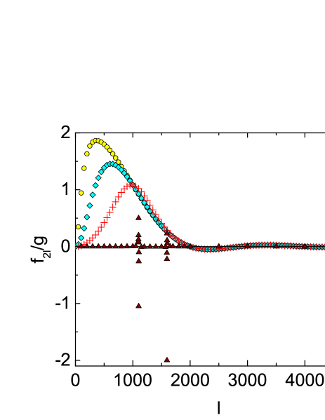
Fig. 1: Values of $f_{2l}/g$ for various $l$ for the 1D system of $N=1000$ ⁴He atoms with interatomic potential (LABEL:p1) and $a=2\,\mbox{\AA}$, $a/\bar{R}=0.5$. The symbols code the different values of $u_{0}=\frac{U_{0}}{1\mathrm{K}\cdot k_{B}}$: $u_{0}=0.1$ (circles), $u_{0}=1$ (diamonds), $u_{0}=10$ (crosses), and $u_{0}=100$ (triangles). The scale factor $g$ is different for different curves: $g=0.1\frac{u_{0}}{N}\frac{a^{2}}{\bar{R}^{2}}$ for $u_{0}=0.1;1;10$ and $g=1$ for $u_{0}=100$. Note that we have changed the value of $|f_{2l}/g|$ for $l=1596$: the figure shows $f_{2l}/g=-2$, but the real value is $f_{2l}/g=-6.35$.

Next, let us consider Eq. (46) with $l=l_{0}$. Substitute $a_{2l\neq 2l_{0}}$ (54) in (46). In this case, $a_{2l_{0}}$ is canceled in Eq. (46), and we obtain the equation for the frequency:

$$\hbar^{2}\omega^{2}(2l_{0})=E^{2}_{B}(k_{2l_{0}})[1+f_{2l_{0}}]-\hbar^{2}\omega^{2}(2l_{0})\delta A_{2l_{0}}(2l_{0}),$$ (59)

Although the formula (57) was obtained for $\delta A_{2l}(2l_{0})$ when $l\neq l_{0}$, we may formally set $l=l_{0}$ in (57). Such a $\delta A_{2l}(2l_{0})$ is denoted in (59) by $\delta A_{2l_{0}}(2l_{0})$. Let us also denote

$$-\hbar^{2}\omega^{2}(2l_{0})\delta A_{2l_{0}}(2l_{0})=q_{2l_{0}}E^{2}_{B}(k_{2l_{0}}),$$ (60)

then (59) takes the form

$$\hbar^{2}\omega^{2}(2l_{0})=E^{2}_{B}(k_{2l_{0}})[1+f_{2l_{0}}+q_{2l_{0}}],$$ (61)

and we get the equation

$$q_{2l_{0}}=-\delta A_{2l_{0}}(2l_{0})[1+f_{2l_{0}}+q_{2l_{0}}]$$ (62)

for the new parameter $q_{2l_{0}}$. In this case $\delta A_{2l_{0}}(2l_{0})$ is given by (57) and depends on $q_{2l_{0}}$.

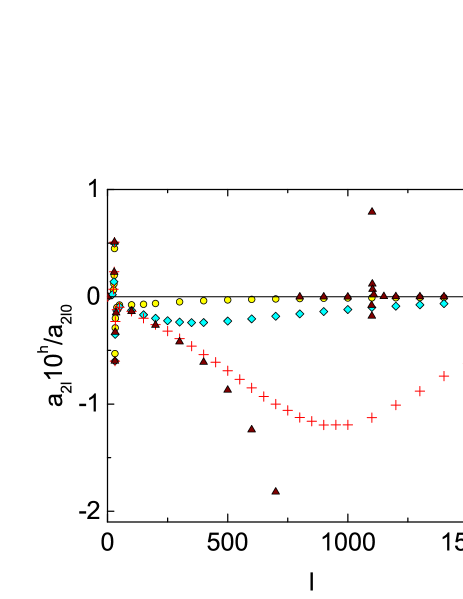
Fig. 2: The set of quantities $a_{2l}(2l_{0})/a_{2l_{0}}(2l_{0})$ for wave packet $\tilde{n}(x)$ (Eqs. (31), (32)) for the $30$th frequency ($l_{0}=30$). The $a_{2l}$ are obtained by the formula (54), where $A_{2l}(2l_{0})=A_{2l}^{(0)}(2l_{0})$ and $A_{2l}^{(0)}(2l_{0})$ is given by (56). Shown are the curves for $u_{0}=0.1$ (circles), $1$ (diamonds), $10$ (crosses), and $u_{0}=100$ (triangles). We consider $N=1000$ ⁴He atoms with interatomic potential (LABEL:p1) for $a=2\,\mbox{\AA}$, $a/\bar{R}=0.5$ and $q_{2l_{0}}=0$. The values of $a_{2l}(2l_{0})$ are multiplied by a factor $10^{h}$, which is equal to $10^{5}$ for $u_{0}=0.1;1;10$. For $u_{0}=100$ we assume $10^{h}=10^{5}$ when $l\leq 750$ and $10^{h}=10$ when $l>750$. The discontinuity in the curve $\blacktriangle\blacktriangle\blacktriangle$ at $l=750$ is fictitious and is only caused by the change in the coefficient $10^{h}$.

It is difficult to analyze analytically the equations obtained, but the numerical analysis is rather simple. We used the “semi-transparent sphere” potential

$$U(|x_{1}-x_{2}|)=\left[\begin{array}[]{ccc}U_{0}>0,&\ |x_{1}-x_{2}|\leq a&\\ 0,&\ a<|x_{1}-x_{2}|\leq L&\end{array}\right.$$ (63)

for the domain $x_{1},x_{2}\in[0,L]$ and solved the system of equations (46) for $l=1,2,\ldots,l^{max}$ ($l^{max}\simeq 10N\bar{R}/a$) and several values of $a/\bar{R}$ and $u_{0}$ (here $u_{0}=\frac{U_{0}}{1\mathrm{K}\cdot k_{B}}$ and $\bar{R}=L/N$ is the mean interatomic distance) using perturbation theory (54)–(62). The summations in (45), (47), (56) and (57) were performed over $p=1,2,\ldots,l^{max}$ and $j=0,\pm 1,\ldots,\pm l^{max}$; increasing $l^{max}$ by a factor of $10$ changes the results negligibly. For ⁴He atoms ($a\approx 2\,\mbox{\AA}$) the numerical analysis shows that the numbers $f_{2l}$ (51) are very small ($|f_{2l}|\ \lower-1.2pt\vbox{\hbox{\hbox to0.0pt{$<$\hss}\lower 5.0pt\vbox{\hbox{$\sim$}}}}\ 1/N$, see fig. 1) when $u_{0}a/\bar{R}\ \lower-1.2pt\vbox{\hbox{\hbox to0.0pt{$<$\hss}\lower 5.0pt\vbox{\hbox{$\sim$}}}}\ 10$. In this case, the largest among $|f_{2l}|$’s is equal to $|f_{2l}|\simeq\frac{0.1u_{0}}{N}\frac{a^{p}}{\bar{R}^{p}}$ with $p\approx 1$–$2$. The inequalities $|a_{2l\neq 2l_{0}}(2l_{0})|\ll|a_{2l_{0}}(2l_{0})|$ and (58) are satisfied provided that $u_{0}a/\bar{R}\ \lower-1.2pt\vbox{\hbox{\hbox to0.0pt{$<$\hss}\lower 5.0pt\vbox{\hbox{$\sim$}}}}\ 1$. Values of $a_{2l}(2l_{0})/a_{2l_{0}}(2l_{0})$ and $\delta A_{2l}(2l_{0})/A^{(0)}_{2l}(2l_{0})$ for different sets of parameters are shown in figures 2 and 3. When $u_{0}a/\bar{R}\gg 1$, several values $a_{2l}(2l_{0})/a_{2l_{0}}(2l_{0})$ and all $\delta A_{2l}(2l_{0})/A^{(0)}_{2l}(2l_{0})$ turn out to be of the order of unity (in modulus), so our perturbation theory does not work. We have checked this for $N=100,1000,10000$ and many values of $l_{0}$.

In the numerical analysis we used $\hbar^{2}\omega^{2}$ (61) with $q$ as a free parameter. We varied $q$ from -100 to 100 and compared it with the theoretical $q$ which is given by the left-hand side of (62). The solution for $q$ is that $q$ for which the theoretical $q$ is equal to a free one. We obtained $|q|\ \lower-1.2pt\vbox{\hbox{\hbox to0.0pt{$<$\hss}\lower 5.0pt\vbox{\hbox{$\sim$}}}}\ 0.01/N$ for $u_{0}a/\bar{R}\ \lower-1.2pt\vbox{\hbox{\hbox to0.0pt{$<$\hss}\lower 5.0pt\vbox{\hbox{$\sim$}}}}\ 1$, $N=100,1000$ and $l_{0}=1,2,\ldots,l^{max}$ with $l^{max}\simeq 10N\bar{R}/a$. Note that (62) is an algebraic equation of infinite degree with respect to $q_{2l_{0}}$. Therefore there must be an infinite number of roots $q_{2l_{0}}$. All the roots except $q_{2l_{0}}=0$ are probably complex.

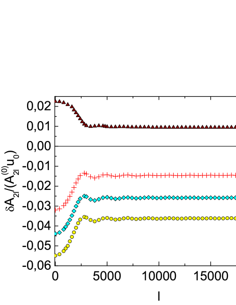
Fig. 3: Values of $\delta A_{2l}(2l_{0})/[A^{(0)}_{2l}(2l_{0})u_{0}]$ for various $l$’s for the system of $N=1000$ ⁴He atoms with interatomic potential (LABEL:p1); $l_{0}=30$, $q_{2l_{0}}=0$, $a=2\,\mbox{\AA}$, and $a/\bar{R}=0.5$. Shown are the curves for $u_{0}=0.1$ (circles), $1$ (diamonds), $10$ (crosses), and $100$ (triangles). The values of $A^{(0)}_{2l}(2l_{0})$ and $\delta A_{2l}(2l_{0})$ are obtained by the formulae (56) and (57).

Thus, the numerical analysis shows that $|f_{2l}|\ \lower-1.2pt\vbox{\hbox{\hbox to0.0pt{$<$\hss}\lower 5.0pt\vbox{\hbox{$\sim$}}}}\ 1/N$ and $|q(2l_{0})|\ \lower-1.2pt\vbox{\hbox{\hbox to0.0pt{$<$\hss}\lower 5.0pt\vbox{\hbox{$\sim$}}}}\ 0.01/N$ for all $l$ and $l_{0}$ provided that $u_{0}a/\bar{R}\ \lower-1.2pt\vbox{\hbox{\hbox to0.0pt{$<$\hss}\lower 5.0pt\vbox{\hbox{$\sim$}}}}\ 1$. In this case, Eq. (61) takes the form

$$\hbar^{2}\omega^{2}(k)=E^{2}_{B}(k),$$ (64)

which is equivalent to the famous Bogoliubov formula (1).

An analysis of the system of equations (48) for odd harmonics also leads to the Bogoliubov dispersion law. In this case formulae and figures are similar, so we will skip them.

As mentioned in the introduction, one of the difficulties in the case of zero BCs is determining the quasimomentum of the quasiparticle. The analysis above allows one to find the quasimomentum. Since $|a_{2l}(2l_{0})/a_{2l_{0}}(2l_{0})|\ll 1$ for all $l_{0}=1,2,\ldots,l^{max}$ and all $l\neq l_{0}$, the harmonic $a_{2l_{0}}$ strongly dominates the wave packet $\tilde{n}(x)$ (31). Therefore the value $k_{2l_{0}}=\pi 2l_{0}/L$ is the quasimomentum of the quasiparticle. Similarly, one can obtain that for an odd harmonic, the quasimomentum is $k_{2l_{0}-1}=\pi(2l_{0}-1)/L$. Thus, we have a general formula for the quasiparticle quasimomentum: $k_{l_{0}}=\pi l_{0}/L$ ($l_{0}=1,2,\ldots,\infty$), which agrees with the results of papers [7, 8, 36, 37].

The question is: have we found all the solutions for the frequencies? The answer is yes. Indeed, the system (46) can be solved for a finite number of $l$: $l=1,2,\ldots,l^{max}$. Equating the corresponding determinant to zero, we obtain an algebraic equation of degree $l$ for $\omega^{2}$. Hence there must be $l^{max}$ solutions. But we found exactly $l^{max}$ values of $\omega^{2}$, corresponding to quasimomenta $k_{2},k_{4},\ldots,k_{2l^{max}}$. So there are no other solutions. Similarly for the system (48).

Note that the exact solution for the ground state energy $E_{0}$ of a 1D system of point bosons ($U(|x_{j}-x_{l}|)=2c\delta(x_{j}-x_{l})$) is close to Bogoliubov’s $E_{0}$ only for $N\ \lower-1.2pt\vbox{\hbox{\hbox to0.0pt{$>$\hss}\lower 5.0pt\vbox{\hbox{$\sim$}}}}\ 1000$ [38, 34]. Since Gross’ approximation $\hat{\Psi}(\textbf{r},t)=\Psi(\textbf{r},t)$ [17] is in fact the zero approximation of Bogoliubov’s approach [1], Gross’ equation (2) can be applied to systems with $N\ \lower-1.2pt\vbox{\hbox{\hbox to0.0pt{$>$\hss}\lower 5.0pt\vbox{\hbox{$\sim$}}}}\ 1000$. The criterion for the applicability of Bogoliubov’s model in the 1D case for zero BCs is $\frac{\sqrt{\gamma}}{2\pi}\ln{\frac{N\sqrt{\gamma}}{\pi}}\ll 1$ (at $T=0$) [8] where $\gamma=\frac{2mc}{\hbar^{2}n}$. This criterion can be written as

$$\gamma\ll b=\left(\frac{2\pi}{\ln{\frac{N\sqrt{\gamma}}{\pi}}}\right)^{2}.$$ (65)

The condition $\gamma\ll b$ is equivalent to $u_{0}\ll 1.5ba/\bar{R}$, since $n=1/\bar{R}$ and $c=\nu(0)/2=U_{0}a$ for the potential (LABEL:p1), and since $a\approx 2\,\mbox{\AA}$, $\hbar^{2}/(2ma^{2})\approx 1.5k_{B}\,\mathrm{K}$ for ⁴He atoms. In order for the system to be uniform far from the walls, the inequality $N\sqrt{\gamma}\gg 1$ should be satisfied [8, 34]. So we have $b\sim 1$ for not too large $N$, and $b\rightarrow 0$ for $N\rightarrow\infty$. The usability condition $u_{0}a/\bar{R}\ \lower-1.2pt\vbox{\hbox{\hbox to0.0pt{$<$\hss}\lower 5.0pt\vbox{\hbox{$\sim$}}}}\ 1$ of the perturbation theory constructed above is equivalent to the condition $u_{0}\ \lower-1.2pt\vbox{\hbox{\hbox to0.0pt{$<$\hss}\lower 5.0pt\vbox{\hbox{$\sim$}}}}\ \bar{R}/a$. For real-world systems we have $\bar{R}/a\geq 1$. According to these estimates, the condition $u_{0}\ll 1.5ba/\bar{R}$ required for Bogoliubov’s approach to work, sets a narrower range of variability of $u_{0}$ as compared to the range $u_{0}\ \lower-1.2pt\vbox{\hbox{\hbox to0.0pt{$<$\hss}\lower 5.0pt\vbox{\hbox{$\sim$}}}}\ \bar{R}/a$, in which our perturbation theory holds. Thus, our method works in the entire range of parameters for which Gross’ equation holds.

Interestingly, Bogoliubov’s solutions for $E_{0}$ and $E(k)$ are valid in a wider range of parameters than the applicability range (65) of Bogoliubov’s method: for a 1D system of point bosons, the exact solutions for the ground state energy $E_{0}$ [38, 39] and the dispersion law $E(k)$ [4, 7] are close to Bogoliubov’s solutions at $\gamma\ \lower-1.2pt\vbox{\hbox{\hbox to0.0pt{$<$\hss}\lower 5.0pt\vbox{\hbox{$\sim$}}}}\ 1,N\gg 1$ (even for $N\rightarrow\infty$, which is inconsistent with the condition (65)). The cause of this is still unclear.

3 Conclusion

We have found the dispersion law of a one-dimensional weakly interacting zero-temperature Bose gas under zero boundary conditions by solving Gross’ equation using the perturbation theory. Such a method is mainly analytical (the numerical analysis is only used to prove the smallness of some quantities and to determine the range of applicability of the method). Note that all frequencies $\omega$ can be found from the systems of equations (46), (48) numerically by setting the determinants of two corresponding matrices to zero. This approach is mostly numerical and is beyond the scope of this article.

Our results show that the dispersion law of a Bose gas with zero BCs coincides with the dispersion law of the same periodic system. A similar result has been obtained previously by other methods [7, 8, 36, 37]. According to an analysis in [40], the ground state energy of a Fermi system is the same for periodic and twisted BCs.