General notions of indexability for queueing control and asset management

Abstract

We develop appropriately generalized notions of indexability for problems of dynamic resource allocation where the resource concerned may be assigned more flexibility than is allowed, for example, in classical multi-armed bandits. Most especially we have in mind the allocation of a divisible resource (manpower, money, equipment) to a collection of objects (projects) requiring it in cases where its over-concentration would usually be far from optimal. The resulting project indices are functions of both a resource level and a state. They have a simple interpretation as a fair charge for increasing the resource available to the project from the specified resource level when in the specified state. We illustrate ideas by reference to two model classes which are of independent interest. In the first, a pool of servers is assigned dynamically to a collection of service teams, each of which mans a service station. We demonstrate indexability under a natural assumption that the service rate delivered is increasing and concave in the team size. The second model class is a generalization of the spinning plates model for the optimal deployment of a divisible investment resource to a collection of reward generating assets. Asset indexability is established under appropriately drawn laws of diminishing returns for resource deployment. For both model classes numerical studies provide evidence that the proposed greedy index heuristic performs strongly.

, and

t1Supported by EPSRC Grant EP/E049265/01. t2Supported by an RCUK Fellowship.

1 Introduction

A notable, now classical, contribution to the theory of dynamic resource allocation was the elucidation by Gittins git79 , git89 of index-based solutions to a large family of multi-armed bandit problems (MABs). This is a class of models concerned with the sequential allocation of effort, to be thought of as a single indivisible resource, to a collection of stochastic reward generating projects (or bandits as they are sometimes called). Gittins demonstrated that optimal project choices are those of highest index. There is no doubt that the idea that strongly performing policies are determined by simple, interpretable calibrations (i.e., indices) of decision options is an attractive and powerful one and offers crucial computational benefits. There is now substantial literature describing extensions to and reformulations of Gittins’ result. Some key contributions are cited in the recent survey of Mahajan and Teneketzis mah07 .

Whittle whi88 introduced a class of restless bandit problems (RBPs) as a means of addressing a critical limitation of Gittins’ MABs, namely, that projects should remain frozen while not in receipt of effort. In RBPs, projects may change state while active or passive though according to different dynamics. However, this generalization is bought at great cost. In contrast to MABs, RBPs are almost certainly intractable having been shown to be PSPACE-hard by Papadimitriou and Tsitsiklis pap99 . Whittle whi88 proposed an index heuristic for those RBPs which pass an indexability test. This heuristic reduces to Gittins’ index policy in the MAB case. Whittle’s index emerges from a Lagrangian relaxation of the original problem and has an interpretation as a fair charge for the allocation of effort to a particular project in a particular state. Weber and Weiss web90 established a form of asymptotic optimality for Whittle’s heuristic under given conditions. More recently, several studies have demonstrated the power of Whittle’s approach in a range of application areas. These include the dynamic routing of customers for service arg08 , gla07 , machine maintenance gla05 , asset management gla06 and inventory routing arc08 .

The above classical models and associated theory are undeniably powerful when applicable. However, the scope of their applicability is heavily constrained by the very simple view the models take of the resource to be allocated. As indicated above, in Gittins’ MAB model a single indivisible resource is allocated wholly and exclusively to a single project at each decision epoch. In Whittle’s RBP formulation, parallel server versions of this are allowed. Many applications, however, call for the allocation of a divisible resource (e.g., money, manpower or equipment) in situations where its over concentration would usually be far from optimal. This is the case, for example, in the problem concerning the planning of new product pharmaceutical research which was discussed by Gittins git89 and which provided practical motivation for his pioneering contribution. This paper records the first outcomes of a major research program whose goal is to develop a usable and effective index theory for such problems.

In Section 2 we present a general model for dynamic resource allocation. Both Gittins’ MABs and Whittle’s RBPs may be recovered as special cases as may the recent model of gla08 which extends Gittins’ MABs such that bandit activation consumes amounts of the available resource which may vary by bandit and state. Our general model allows for resource to be applied at a range of levels to each constituent project, subject to some overall constraint on the total rate at which resource is available. A notion of (full) indexability which generalizes that of Whittle for RBPs is developed. Any project which is fully indexable has an index which is a function both of a given resource level ($a$) and of a given state ($x$). The index $W(a,x)$ may be understood as a fair charge for raising the project’s resource level above $a$ when in state $x$. We discuss how to use such indices to develop heuristics for dynamic resource allocation when all projects are fully indexable.

In Sections 3 and 4 we use the ideas and methods of Section 2 to construct index heuristics for the dynamic allocation of a divisible resource in the context of two model classes which are of considerable interest in their own right. In Section 3 we deploy the framework of Section 2 to develop heuristics for the dynamic allocation of a pool of $S$ servers to $K$ service stations (or customer classes) at which queues may form. This model is able to capture situations where, for example, each of $K$ customer classes is served by a dedicated team of specialists. Additionally, $S$ higher level generalist servers are available for deployment across the customer classes to supplement the specialist teams as demand dictates. Deployment of $a_{k}$ generalists to customer class $k$ enhances the local specialist team which then delivers service collectively at rate $\mu_{k}(a_{k})$. An assumption that the service rate functions $\mu_{k}$ are increasing and concave reflects a law of diminishing returns as service teams grow. The problem of determining how the pool of generalists should be deployed across the customer classes in response to queue length information is formulated as a dynamic resource allocation problem of the kind discussed in Section 2. The analysis which establishes full indexability in Section 3 markedly adds to the queueing control literature in establishing monotonicity with respect to service costs of optimal policies for a derived problem involving a single queue. An algorithm is given for the computation of indices. A numerical study provides evidence that a greedy index heuristic for allocating the common service pool is close to optimal throughout a numerical study featuring nearly 10,000 two station problems.

The model class studied in Section 4 generalizes the so-called spinning plates model discussed by Glazebrook, Kirkbride and Ruiz-Hernandez gla06 . It is a flexible finite state model class in which a divisible investment resource is available to drive improvements to the (reward) performance of $K$ reward generating assets, which in the absence of any such resource deployment will tend to deteriorate. Positive investment both arrests an asset’s tendency to deteriorate and enhances asset performance by enabling movement of the asset state toward those in which its reward generating performance will be stronger. Full indexability for assets is established under laws of diminishing returns as asset investment levels grow. This considerably extends the work of Glazebrook, Kirkbride and Ruiz-Hernandez gla06 . A numerical study which features 14,000 two asset problems testifies to the strong performance of the greedy index heuristic in comparison to optimum and to competitor policies. Conclusions and proposals for further work are discussed in Section 5.

2 A model for dynamic resource allocation

We propose a semi-Markov decision process (SMDP) formulation $\{(\Omega_{k},L_{k},c_{k},r_{k},q_{k}),1\leq k\leq$ $K\}$ of the problem of dynamically allocating a resource to a collection of $K$ stochastic projects. This formulation includes Gittins’ MABs and Whittle’s RBPs as special cases. In our SMDP project $k$ is characterized by its (finite or countable) state space $\Omega_{k}$, its highest activation level $L_{k}\in\mathbb{Z}^{+}$, cost rate function $c_{k}\dvtx\{0,1,\ldots,L_{k}\}\times\Omega_{k}\rightarrow\mathbb{R}^{+}$, resource consumption function $r_{k}\dvtx\{0,1,\ldots,\break L_{k}\}\times\Omega_{k}\rightarrow\mathbb{R}^{+}$ and Markov transition law $q_{k}$. The model is in continuous time. We use $x_{k},x_{k}^{\prime}\in\Omega_{k}$ for generic states of project $k$ and $\mathbf{x},\mathbf{x}^{\prime}\in\mathop{\mbox{{$\!\times$}}}_{k=1}^{K}\Omega_{k}$ for generic states of the process. In the SMDP an action $\mathbf{a}=(a_{1},a_{2},\ldots,a_{K})$ must be taken at time $0$ and after each (state) transition of the process. This specifies the resource level $a_{k}\in\{0,1,\ldots,L_{k}\}$ to be applied to project $k,1\leq k\leq K$. The choice $a_{k}=0$ indicates that resource at a minimal level (usually none) is to be applied to $k$ ($k$ is passive), while the choice $a_{k}=L_{k}$ indicates a maximal resource allocation. Resource level $a_{k}$ applied to project $k$ when in state $x_{k}$ leads to a consumption of resource at rate $r_{k}(a_{k},x_{k})$, with $r_{k}(\cdot,x_{k})$ increasing $\forall k,x_{k}$. In the major examples discussed in the upcoming sections we will have $r_{k}(a_{k},x_{k})=a_{k}$ $\forall k,x_{k}$ and the resource level is identified with the resource consumed. When resource level $a_{k}$ is applied to project $k$ when in state $x_{k}$, it incurs costs at rate $c_{k}(a_{k},x_{k})$. Both cost and resource consumption rates are additive over projects. It will be convenient to write $c(\mathbf{a},\mathbf{x})=\sum_{k}c_{k}(a_{k},x_{k})$ and $r(\mathbf{a},\mathbf{x})=\sum_{k}r_{k}(a_{k},x_{k})$. The set of admissible actions in process state $\mathbf{x}$ is given by $A(\mathbf{x})=\{\mathbf{a};r(\mathbf{a},\mathbf{x})\leq R\}$ where $R$ is the rate at which resource is available to the system, assumed constant over time. We suppose that $A(\mathbf{x})\neq\phi,\mathbf{x}\in\mathop{\mbox{{$\!\times$}}}_{k=1}^{K}\Omega_{k}$. An admissible policy is a rule for taking admissible actions.

Should action $\mathbf{a}$ be taken when the system is in state $\mathbf{x}$, the system will remain in state $\mathbf{x}$ for an amount of time which is exponentially distributed with rate

$$\sum_{\mathbf{x}^{\prime}\in\mathop{\mbox{{$\!\times$}}}_{k}\Omega_{k}}\mathbf{q}(\mathbf{x}^{\prime}\mid\mathbf{x},\mathbf{a})=\sum_{k=1}^{K}\sum_{x_{k}^{\prime}\in\Omega_{k}}q_{k}(x_{k}^{\prime}\mid x_{k},a_{k})\leq Q<\infty\qquad\forall\mathbf{x},\mathbf{a}.$$

The transition following will be from state $x_{k}$ to state $x_{k}^{\prime}$ within project $k$ with probability

$$q_{k}(x_{k}^{\prime}\mid x_{k},a_{k})\biggl{\{}\sum_{\mathbf{x}^{\prime}\in\,\mathop{\mbox{{$\!\times$}}}_{k}\mathbf{\Omega}_{k}}\mathbf{q}(\mathbf{x}^{\prime}\mid\mathbf{x},\mathbf{a})\biggr{\}}^{-1}.$$

Hence the projects evolve independently, given the choice of action, with $q_{k}$ yielding transition rates for project $k$. The goal of analysis is the determination of a policy for resource allocation (a rule for taking admissible actions at all decision epochs) which minimizes the average cost per unit time incurred over an infinite horizon.

To develop ideas and notation we use $\bar{\mathbf{U}}$ for the set of deterministic, stationary, Markov (DSM) and admissible policies determined by functions $\mathbf{u}$ with domain $\mathop{\mbox{{$\!\times$}}}_{k=1}^{K}\Omega_{k}$ which satisfy $\mathbf{u}(\mathbf{x})\in A(\mathbf{x})$ $\forall\mathbf{x}$. Fix $\mathbf{u}\in\bar{\mathbf{U}}$. We shall also use $\{\mathbf{X}(t),t\geq 0\}$ for the system state evolving over time and $[\mathbf{u}\{\mathbf{X}(t)\},t\geq 0]$ for the corresponding stochastic process of admissible actions taken by $\mathbf{u}$. We write

$$C(\mathbf{u},\mathbf{x})=\mathop{\lim\inf}_{t\rightarrow\infty}\frac{1}{t}\biggl{(}\int_{0}^{t}\mathbb{E}_{\mathbf{u}}^{\mathbf{x}}c(\mathbf{u}\{\mathbf{X}(s)\},\mathbf{X}(s))\,ds\biggr{)}$$ (1)

for the average cost per unit time incurred under policy $\mathbf{u}$ over an infinite horizon from initial state $\mathbf{x}$. In (1) $\mathbb{E}_{\mathbf{u}}^{\mathbf{x}}$ denotes an expectation taken over realizations of the system evolving under $\mathbf{u}$ from initial state $\mathbf{x}$. We shall assume the existence of a policy $\mathbf{u}\in\bar{\mathbf{U}}$ such that $C(\mathbf{u},\mathbf{x})<\infty$ $\forall\mathbf{x}$ and write $C^{\mathrm{opt}}(\mathbf{x})$ for the minimized cost rate, namely,

$$C^{\mathrm{opt}}(\mathbf{x})=\inf_{\mathbf{u}\in\bar{\mathbf{U}}}C(\mathbf{u},\mathbf{x}).$$ (2)

We shall use the term optimal to denote a policy (assumed to exist) which achieves the infimum in (2) uniformly over initial states. This applies both to the problem in (2) and also to the derived optimization problems we shall discuss later in the account. In the model classes featured in Sections 3 and 4 it will be the case that the average costs in (1) and (2) are independent of $\mathbf{x}$. Henceforth, for simplicity, we shall suppress dependence on the initial state $\mathbf{x}$ in the notation.

We shall use

$$R(\mathbf{u})=\mathop{\lim\inf}_{t\rightarrow\infty}\frac{1}{t}\biggl{(}\int_{0}^{t}\mathbb{E}_{\mathbf{u}}r(\mathbf{u}\{\mathbf{X}(s)\},\mathbf{X}(s))\,ds\biggr{)}$$ (3)

for the average rate at which resource is consumed under policy $\mathbf{u}$. We also write

$$C(\mathbf{u})=\sum_{k=1}^{K}C_{k}(\mathbf{u}),\qquad R(\mathbf{u})=\sum_{k=1}^{K}R_{k}(\mathbf{u})$$ (4)

to give a disaggregation of the cost and resource consumption rates into the contributions from individual projects.

In principle, the tools of dynamic programming (DP) are available to determine optimal policies. See, for example, put94 . However, direct application of DP is computationally infeasible other than for small problems (crucially, small $K$). Hence, our primary interest lies in the development of heuristic policies which are close to cost minimizing. To this end we relax the optimization problem in (2) by extending the class of policies from the DSM admissible class $\bar{\mathbf{U}}$ to those DSM policies $\mathbf{u}\dvtx\mathop{\mbox{{$\!\times$}}}_{k=1}^{K}\Omega_{k}\rightarrow\mathop{\mbox{{$\!\times$}}}_{k=1}^{K}\{0,1,\ldots,L_{k}\}$ which consume resource at an average rate which is no greater than $R$. Hence, we write

$$\acute{C}^{\mathrm{opt}}=\inf_{\mathbf{u}}\sum_{k=1}^{K}C_{k}(\mathbf{u}),$$ (5)

where in (5), the infimum is taken over the collection of DSM policies satisfying

$$\sum_{k=1}^{K}R_{k}(\mathbf{u})\leq R.$$ (6)

We now relax the problem again by further extending the class of policies and by incorporating the constraint (6) into the objective (5) in a Lagrangian fashion. We write

$$C(W)=\inf_{\mathbf{u}}\sum_{k=1}^{K}\{C_{k}(\mathbf{u})+WR_{k}(\mathbf{u})\}-WR.$$ (7)

In (7) the infimum is taken over the class of DSM policies $\mathbf{u}\dvtx\mathop{\mbox{{$\!\times$}}}_{k=1}^{K}\Omega_{k}\rightarrow\mathop{\mbox{{$\!\times$}}}_{k=1}^{K}\{0,1,\ldots,L_{k}\}$ which allow, for each project $k$, a free choice of action from the set $\{0,1,\ldots,L_{k}\}$ at each decision epoch. It is clear that

$$C(W)\leq\acute{C}^{\mathrm{opt}}\leq C^{\mathrm{opt}},\qquad W\in\mathbb{R}^{+}.$$

However, the Lagrangian relaxation of our optimization problem expressed by (7) admits, on account both of the policy class involved and the nature of the objective, an additive project-based decomposition. Expressed differently, an optimal policy for (7) operates optimal policies for the individual projects in parallel. In an obvious notation we write

$$C(W)=\sum_{k=1}^{K}C_{k}(W)-WR,$$ (8)

where

$$C_{k}(W)=\inf_{u_{k}}\{C_{k}(u_{k})+WR_{k}(u_{k})\},\qquad 1\leq k\leq K.$$ (9)

The optimization problem in (9) concerns project $k$ alone. We denote it $P(k,W)$. In its objective the Lagrange multiplier $W$ plays the role of a charge per unit of time and per unit of resource consumed. An optimal policy $u_{k}(W)$ for $P(k,W)$ minimizes an aggregate rate of project costs incurred and charges levied for resource consumed. Further, the policy $\mathbf{u}(W)$ which applies $u_{k}(W)$ to each project $k$, achieves $C(W)$ in (7) and hence provides a solution to the above Lagrangian relaxation. Note that in what follows we shall use the notation $\mathbf{u}(W,\mathbf{x}),u_{k}(W,x_{k})$ to denote the action (resource consumption levels) chosen by DSM policies $\mathbf{u}(W),u_{k}(W)$ in states $\mathbf{x},x_{k}$, respectively.

In order to develop natural project calibrations (or indices) which can facilitate the construction of effective heuristics for our original problem (2), we seek optimal policies for the problems $\{P(k,W),W\in\mathbb{R}^{+},1\leq k\leq K\}$ which are structured as in Definition 1 below. We first require additional notation. Write

$$\quad\Pi_{k}\{u_{k}(W),a\}=\{x\in\Omega_{k};u_{k}(W,x)\leq a\},\qquad a\in\{0,1,\ldots,L_{k}-1\},$$ (10)

for the set of project $k$ states for which policy $u_{k}(W)$ chooses to consume resource at level $a$ or below.

Definition 1 ((Full indexability)).

Project $k$ is fully indexable if there exists a family of DSM policies $\{u_{k}(W),W\in\mathbb{R}^{+}\}$ such that $u_{k}(W)$ is optimal for $P(k,W)$ $\forall W$ and $\Pi_{k}\{u_{k}(W),a\}$ is nondecreasing in $W$ for each $a\in\{0,1,\ldots,L_{k}-1\}$.

To summarize the requirements of Definition 1, a project $k$ will be fully indexable if the problem $P(k,W)$ has an optimal policy which, for any given state, consumes an amount of resource which is decreasing in the resource charge $W$. Full indexability enables a calibration of the individual projects as described in Definition 2.

Definition 2 ((Project indices)).

If project $k$ is fully indexable as in Definition 1, a corresponding index function $W_{k}\dvtx\{0,1,\ldots,L_{k}-1\}\times\Omega_{k}\rightarrow\mathbb{R}^{+}$ is given by

$$W_{k}(a,x)=\inf[W;x\in\Pi_{k}\{u_{k}(W),a\}].$$ (11)

The index $W_{k}(a,x)$ can be thought of as a fair charge at project $k$ for raising the resource level from $a$ to $a+1$ in state $x$. Were a resource charge less than $W_{k}(a,x)$ to be levied, the consumption of the additional resource would be preferable, while if the resource charge were to be in excess of the index, that would not be the case. We shall adopt the convention that the index function is extended to $W_{k}\dvtx\{-1,0,1,\ldots,L_{k}\}\times\Omega_{k}\rightarrow\mathbb{R}^{+}\cup\{\infty\}$ where $W_{k}(-1,x)=\infty,W_{k}(L_{k},x)=0$ $\forall x\in\Omega_{k}$.

The following is a simple consequence of the above definitions. Its proof is omitted.

Lemma 1

If project $k$ is fully indexable, the index $W_{k}(a,x)$ is decreasing in $a$, for fixed $x$.

Hence, under full indexability, the fair charge for raising the resource level for project $k$ in any state $x$ from $a$ to $a+1$ is decreasing in the resource level $a$.

We now return to consideration of the Lagrangian relaxation in (7) and (8) and suppose that all $K$ projects are fully indexable with families of optimal policies

$$\{u_{k}(W),W\in\mathbb{R}^{+},1\leq k\leq K\}$$

structured as in Definition 1. Under full indexability, all of these policies have a structure describable in terms of the index functions $W_{k},1\leq k\leq K$. Theorem 2 now follows.

Theorem 2

Suppose that all $K$ projects are fully indexable with extended index functions $W_{k}\dvtx\{-1,0,1,\ldots,L_{k}\}\times\Omega_{k}\rightarrow\mathbb{R}^{+}\cup\{\infty\}$. The policy $\mathbf{u}(W)$ such that

$$\mathbf{u}(W,\mathbf{x})=\mathbf{a}\quad\Longleftrightarrow\quad W_{k}(a_{k}-1,x_{k})>W\geq W_{k}(a_{k},x_{k}),$$ (12)

$$\eqntext{1\leq k\leq K,\mathbf{x}\in\mathop{\mbox{{$\!\times$}}}_{k=1}^{K}\Omega_{k},}$$

achieves $C(W)$ $\forall W\in\mathbb{R}^{+}$.

According to Theorem 2, policy $\mathbf{u}(W)$ constructs actions (allocations of resource) in each system state by accumulating resource at each project until the fair charge for adding further resource drops below the prevailing charge $W$. This is strongly suggestive of how effective, interpretable heuristics for our original dynamic resource allocation problem based on the above indices (fair charges) may be constructed when all projects are fully indexable. A natural greedy index heuristic constructs actions in every system state by increasing resource consumption levels in decreasing order of the above station indices until the point is reached when the resource constraint is violated by additional allocation of resource.

Formally the greedy index heuristic is structured as follows:

Greedy index heuristic

In state $\mathbf{x}$ the greedy index heuristic constructs an action (allocation of resource) as follows:

Step 1. The initial allocation is $\mathbf{0}=\{0,0,\ldots,0\}$. The current allocation is $\mathbf{a}=\{a_{1},a_{2},\ldots,a_{K}\}$ with $\sum_{k}r_{k}(a_{k},x_{k})<R$.

Step 2. Choose any $k$ satisfying

$$W_{k}(a_{k},x_{k})=\max_{1\leq j\leq K}W_{j}(a_{j},x_{j}).$$

Step 3. If $\mathbf{e}_{k}$ denotes a $K$-vector whose $k$th component is 1 with zeroes elsewhere, the new deployment is $\mathbf{a}+\mathbf{e}_{k}$ if

$$\sum_{l\neq k}r_{l}(a_{l},x_{l})+r_{k}(a_{k}+1,x_{k})\leq R.$$ (13)

If there is strict inequality in (13), return to Step 1 and repeat. Otherwise, stop and declare $\mathbf{a}+\mathbf{e}_{k}$ to be the chosen action in $\mathbf{x}$. If

$$\sum_{l\neq k}r_{l}(a_{l},x_{l})+r_{k}(a_{k}+1,x_{k})>R,$$

stop and declare $\mathbf{a}$ to be the chosen action in $\mathbf{x}$. We shall use Figure 1 to illustrate the construction of actions by both the policy $\mathbf{u}(W)$ (as in Theorem 2) and the greedy index heuristic in a simple problem with $K=2$ in which both projects are fully indexable. Section 3 discusses a class of models in which $r_{k}(a_{k},x_{k})=a_{k}$ $\forall k,x_{k}$ and where all projects have state space $\mathbb{N}$ and a common maximum resource level, $L$ say, which is equal to $R$, the total rate at which resource is available. Suppose now that $L=R=5$ in such a model and that the system state is $\mathbf{x}=(x_{1},x_{2})=(5,2)$. Figure 1 indicates values of the appropriate project indices $W_{1}(a,5)$ and $W_{2}(a,2)$ for the range $0\leq a\leq 4$ together with the value of the Lagrange multiplier $W$.

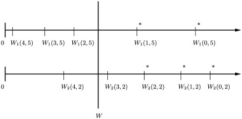
Figure 1: Index values for state $\mathbf{x}=(5,2)$.

The policy $\mathbf{u}(W)$ will make allocations of resource supported by those index values which are above $W$. Hence from Figure 1, the choice of action in state $\mathbf{x}=(5,2)$ will be $\mathbf{a}=(2,4)$. This is an inadmissible action for the original problem since the total resource rate allocated (6) exceeds that available (5). The greedy heuristic makes allocations of resource supported by the five largest index values (indicated by $*$ in Figure 1). Plainly, the action taken by the index heuristic is $\mathbf{a}=(2,3)$. As the system state evolves under the operation of either policy, the index values change as do the implied actions.

The major challenge to implementation of the above program for heuristic construction is the identification of optimal policies for the problems

$$\{P(k,W),1\leq k\leq K,W\in\mathbb{R}^{+}\},$$

which meet the requirements of Definition 1. In Sections 3 and 4 we are able to achieve this in the context of two model classes for which we are able to establish an appropriate form of full indexability. For the Section 3 problem, we also give an algorithm for index computation. For both model classes we proceed to assess the performance of the greedy index heuristic in extensive numerical studies.

We recover Whittle’s RBPs whi88 by making the choices $r_{k}(a_{k}$, $x_{k})=a_{k},L_{k}=1,1\leq k\leq K$ and $R<K$ in the above. Hence there are just two modes of activation (active, passive) of each project, with $R$ projects to be made active at each epoch. For this special case the above greedy index heuristic is precisely the index heuristic proposed by Whittle. If we make the further choice $R=1$ and impose the requirement that projects can only change state under the active action, we then recover Gittins’ MAB git79 and its associated (optimal) index policy.

3 The optimal allocation of a pool of servers

We illustrate the above ideas by considering a set-up in which service is provided at $K$ service stations. These stations could represent distinct geographical locations or facilities dedicated to the service of a particular class of customer. Customers arrive at the stations in $K$ independent Poisson streams, with $\lambda_{k}$ the rate for station $k$. A pool of $S$ servers is available to support service at the $K$ stations. Should $a$ servers from the pool be allocated to station $k$ at any point, the resulting exponential service rate is $\mu_{k}(a)$. Note that there may be a local team of servers permanently stationed at $k$ (i.e., in addition to any allocated from the pool) in which case we will have $\mu_{k}(0)>0$. Please note also that we shall suppose that all servers (whether permanently based at a location or allocated there from the common pool) offer service as a team, namely, that they act in concert as a single server. The goal of analysis is the determination of a policy for deploying the common service pool in response to queue length information to minimize some linear measure of holding cost rate for the system incurred over an infinite horizon.

More formally, the system state at time $t$ is $\mathbf{n}(t)=\{n_{1}(t),n_{2}(t),\ldots,n_{K}(t)\}$ where $n_{k}(t)$ is the number of customers at service station $k$ (including any in service) at $t$. We shall on occasion refer to $n_{k}(t)$ as the head count at station $k$ at time $t$. This system state is observed continuously. The decision epochs for the system are time zero and the times at which the system state changes. At each decision epoch, some action $\mathbf{a}=(a_{1},a_{2},\ldots,a_{K})$ is taken, where $a_{k}\in\mathbb{N},1\leq k\leq K$, and $\sum_{k}a_{k}\leq S$. Action $\mathbf{a}$ denotes the deployment of $a_{k}$ servers from the central pool to service station $k,1\leq k\leq K$. Should action $\mathbf{a}$ be taken in state $\mathbf{n}$ then an exponentially distributed amount of time with rate

$$\Lambda=\sum_{k}\{\lambda_{k}+\mu_{k}(a_{k})I(n_{k}>0)\}$$ (14)

will elapse before a change of state. In (14) $I$ is an indicator function. The next state of the system will be $\mathbf{n}+\mathbf{e}_{k}$ with probability $\lambda_{k}/\Lambda$ and will be $\mathbf{n}-\mathbf{e}_{k}$ with probability $\mu_{k}(a_{k})I(n_{k}>0)/\Lambda,1\leq k\leq K$.

A DSM admissible policy is given by a map $\mathbf{u}\dvtx\mathbb{N}^{K}\rightarrow\Xi$, where

$$\Xi=\biggl{\{}\mathbf{a};a_{k}\in\mathbb{N},1\leq k\leq K,\mbox{ and }\sum_{k}a_{k}\leq S\biggr{\}}$$ (15)

and is a rule for choosing admissible actions as a function of the current system state. The cost associated with policy $\mathbf{u}$ is given by

$$C(\mathbf{u})=\sum_{k}h_{k}N_{k}(\mathbf{u}),$$ (16)

where the $h_{k}$ are positive weights (holding cost rates) and $N_{k}(\mathbf{u})$ is the time average number of customers at station $k$ under policy $\mathbf{u}$. The optimization problem of interest is given by

$$C^{\mathrm{opt}}=\inf_{\mathbf{u}\in\bar{\mathbf{U}}}C(\mathbf{u}),$$ (17)

where in (17) the infimum is over the set $\bar{\mathbf{U}}$ of DSM admissible policies.

We pause to note that this problem does indeed belong to the class of dynamic resource allocation problems described in the preceding section. We make the choices $c_{k}(a_{k},n_{k})=h_{k}n_{k},r_{k}(a_{k},n_{k})=a_{k},L_{k}=S,1\leq k\leq K$, with the transition rates $q_{k}(n_{k}^{\prime}\mid n_{k},a_{k})$ satisfying

$$q_{k}(n_{k}+1\mid n_{k},a_{k}) = \lambda_{k},$$

$$q_{k}(n_{k}-1\mid n_{k},a_{k}) = \mu_{k}(a_{k})I(n_{k}>0),$$

for all choices of $k,n_{k}$ and $a_{k}$. They are otherwise zero. One thing which is special about this problem is that it is possible to utilize all of the resource which is on offer all of the time. It is plainly optimal to do so. Hence, in (15), we can restrict admissible actions to those which deploy all servers from the pool.

Before proceeding to develop appropriate notions of full indexability/indices, we describe assumptions we shall make about our service rate functions $\mu_{k}(\cdot)$. In Assumption 1 we use the notation

$$\lceil x\rceil=\min\{y;y\in\mathbb{Z}^{+}\mbox{ and }y>x\},\qquad x\in\mathbb{R}^{+}.$$

Assumption 1.

There exist functions $\tilde{\mu}_{k}\dvtx\mathbb{R}^{+}\rightarrow\mathbb{R}^{+}$ which are strictly increasing, twice differentiable and strictly concave, satisfying

$$\tilde{\mu}_{k}(a)=\mu_{k}(a),\qquad a\in[0,S]\cap\mathbb{N},$$ (18)

and

$$\sum_{k=1}^{K}\lceil\tilde{\mu}_{k}^{-1}(\lambda_{k})\rceil<S.$$ (19)

From (18) the functions $\tilde{\mu}_{k},1\leq k\leq K$, are smooth extrapolations of the service rates on the integers in the range $[0,S]$. The properties of these functions reflect the fact that, while an increase in the size of the team at a station results in a higher service rate, the marginal benefit of adding an additional member diminishes as the team size grows. Requirement (19) guarantees the existence of stable policies under which all queue lengths remain finite. It is the assumption of strict concavity of the service rate functions at each station which stimulates an active approach to the distribution of the pool of servers around the stations and which makes this an interesting problem. Had we assumed, for example, that the service rates were all convex in the team size, then sob82 shows that in an optimal policy the service pool would always be allocated en bloc and we are driven back to the “single server” world of the simple bandit models. This result is intuitively obvious, as observed by Richard Serfozo to Sobel: “the fastest rate is also the cheapest.” Indeed, the resulting service control problem has a well-known solution in the form of the so-called $c\mu$-rule. (See coxsmith61 .)

We are able to develop a Lagrangian relaxation of the problem in (16) and (17) as in the preceding section. As in the analysis of Section 2 up to (8), such a relaxation yields $K$ optimization problems $P(k,W)$, one for each station, which here take the form

$$C_{k}(W)=\inf_{u_{k}}\{h_{k}N_{k}(u_{k})+WS_{k}(u_{k})\},$$ (20)

where in (20), the infimum is over the class of DSM policies $u_{k}\dvtx\mathbb{N}\rightarrow\{0,1,\ldots,\break S\}$ which can deploy any number of servers (up to $S$) at station $k$ at each epoch, $N_{k}(u_{k})$ is the time average head count and $S_{k}(u_{k})$ the time average number of servers deployed at $k$ under policy $u_{k}$. The optimization problem in (20) concerns station $k$ alone and seeks to choose, at each station $k$ decision epoch and in response to queue length information for station $k$, the number of servers (from the $S$ available) to be deployed there. The goal is to make such choices to minimize costs which are an aggregate of those incurred through customers waiting $[h_{k}N_{k}(u_{k})]$ and charges imposed for the provision of service $[WS_{k}(u_{k})]$. Note that Lagrange multiplier $W$ here has an economic interpretation as the charge imposed per server per unit of time.

We now wish to develop index heuristics for our service allocation problem by developing station indices of the form described in the preceding section. These flow from the property of full indexability defined with respect to solutions to the problems $P(k,W),1\leq k\leq K$, and described in Definition 1. However, full indexability is a property of individual stations and hence we now focus on a single station and drop the station identifier $k$ until further notice. For clarity, the single station problem $P(W)$ is formulated as an SMDP as follows:

1. The state of the system at time $t\in\mathbb{R}^{+}$ is $n(t)$, the number of customers (head count) at the station. New customers arrive at the station according to a Poisson process of rate $\lambda$.

2. Decision epochs occur at time 0 and whenever there is a change of state. At each such epoch an action from the set $A\equiv\{0,1,\ldots,S\}$ is chosen. Should action $a\in A$ be chosen at time $t$ at which point $n(t)=n>0$ then costs will be incurred from $t$ at rate $hn+Wa$ and the first event following $t$ will occur at time $t+X$ where $X\sim\exp[\lambda+\mu(a)]$. With probabilities $\lambda[\lambda+\mu(a)]^{-1}$ and $\mu(a)[\lambda+\mu(a)]^{-1}$ the event will be, respectively, an arrival or a service completion.

3. The goal of analysis will be the determination of a stationary policy to minimize the average cost rate incurred over an infinite horizon. Trivially, optimal policies offer no service $(a=0)$ when the system is empty $[n(t)=0]$.

The quest for full indexability is greatly simplified in this case by the existence of optimal policies for $P(W)$ for which the choice of number of servers is increasing in the current head count. We call such policies monotone. This conclusion follows from Theorem 4 in Stidham and Weber stidweb89 , which applies to a queueing system with state space $\mathbb{N}$ and Poisson arrivals with an objective which combines a holding cost which is both increasing in the state and unbounded, with action costs which are nonnegative and increasing in the resource level. All of these requirements hold in $P(W)$. Stidham and Weber’s analysis first considers the problem of choosing a policy to minimize the expected cost incurred in moving the system from a general initial state to the empty state (their Theorem 2) and then deploys arguments from renewal theory to demonstrate that such a policy will also minimize long run average costs (their Section 1.3). We state our conclusion as Proposition 3.

Proposition 3 ((Stidham and Weber))

There exists a monotone policy which is optimal for $P(W)$.

The problem of establishing monotonicity with respect to queue size of optimal policies for service control problems for queues with Poisson input is not new. In addition to Stidham and Weber stidweb89 , see crab72 , doshi78 , gall79 , geohar01 , mit73 . While such monotonicity is helpful in establishing full indexability and in the subsequent computation of index functions, it is not the key to proving the latter. This is rather the demonstration (to which we now proceed in Section 3.1) that optimal policies for $P(W)$ are monotone in $W$. Proving this significantly extends the literature on service control problems for $M/M/1$ queues.

3.1 Stations are fully indexable

In light of Proposition 3 we can recast and simplify the requirements of full indexability expressed in Definition 1. Let $u(W)$ be an optimal policy for $P(W)$ which is monotone. It follows that for all choices of $W\in\mathbb{R}^{+}$ and $0\leq a\leq S-1$,

$$\Pi\{u(W),a\}\equiv\{n\in\mathbb{N};u(W,n)\leq a\}=\{0,1,\ldots,N(a,W)\}$$

for some $N(a,W)\in\mathbb{N}\cup\{\infty\}$. We now have the following:

Definition 3 ((Full indexability)).

The station will be fully indexable if there exists a family of DSM policies $\{u(W),W\in\mathbb{R}^{+}\}$ for which (i) $u(W)$ is monotone and optimal for $P(W)$ $\forall W\in\mathbb{R}^{+}$ and (ii) the corresponding $N(a,W)$ is increasing in $W,\forall a\in\{0,1,\ldots,S-1\}$.

To summarize the requirements of Definition 3, a station will be fully indexable if the service charge problem $P(W)$ has a monotone optimal policy for which the number of servers deployed is decreasing in the service charge $W$ for any given head count. Full indexability enables a calibration of the individual stations as described in Definition 4.

Definition 4 ((Station indices)).

If the station is fully indexable, the corresponding index function $W\dvtx\{0,1,\ldots,S-1\}\times\mathbb{N}\rightarrow\mathbb{R}^{+}$ is given by

$$W(a,n)=\inf\{W;n\leq N(a,W)\}.$$ (21)

In light of Proposition 3 above, Lemma 1 may be extended as follows in this case:

Lemma 4

If the station is fully indexable, the index $W(a,n)$ is (i) decreasing in $a$ for fixed $n$ and (ii) increasing in $n$ for fixed $a$.

Please note that optimal policies for $P(W)$ will be unchanged if all cost rates (both holding costs and service charges) are divided by $W>0$ throughout. When we do that, we see that increasing $W$ is equivalent to decreasing the holding cost rate $h$ in problems for which the service charge rate is fixed. This being so, we develop the following convenient reformulation of the definition of full indexability above: refer to the problem obtained by setting $W=1$ in the above [namely $P(1)$] as $Q(h)$ to emphasize dependence on the holding cost parameter $h$. Hence, $Q(h)$ is the problem given by

$$\hat{C}(h)=\inf_{u}\{hN(u)+S(u)\}.$$

From Proposition 3 we are able to assert the existence of optimal policies for $Q(h)$ which are monotone. The following is trivially equivalent to Definition 3 above.

Definition 5 ((Full indexability—alternative definition)).

The station will be fully indexable if there exists a family of DSM policies $\{u(h),h\in\mathbb{R}^{+}\}$ such that, (i) $u(h)$ is optimal for $Q(h)$ $\forall h\in\mathbb{R}^{+}$; (ii) each $u(h)$ is monotone with

$$\Pi\{u(h),a\}=\{0,1,\ldots,M(a,h)\},$$

where $M(a,h)$ is deceasing in $h$ $\forall a\in\{0,1,\ldots,S-1\}$.

To summarize, to achieve full indexability, instead of requiring (according to Definition 3) that the optimal service level decreases with the service charge $W$ (for a fixed value of the holding cost rate $h$), we now equivalently require it to increase with the holding cost rate $h$ (for fixed service charge $W=1$). This reformulation of full indexability which focuses attention on the holding cost element of the objective yields a more accessible account.

We begin this part of our analysis by noting that it is easy to establish that any optimal policy $u(h)$ for $Q(h)$ must be such that $\mu\{u(h,n)\}>0,n\geq 1$. It follows that the head count process is ergodic under its operation. We uniformize station evolution by rescaling time such that

$$\lambda+\mu(S)=1.$$

Under this uniformization, the DP optimality equations for the problem $Q(h)$ are as follows:

$$\qquad\lambda v(h,n) = hn+\lambda v(h,n+1)$$

$${}+\min_{a}\{a-\mu(a)[v(h,n)-v(h,n-1)]\}-\gamma(h),\qquad n\geq 1,$$

where the minimum in (3.1) is over the range $0\leq a\leq S$. Note that in (3.1) the quantity $\gamma(h)$ is the minimized cost rate for $Q(h)$ with $v(h,\cdot)$ the corresponding bias function, where $v(h,0)=0$. If we write $\hat{C}(h,n,t)$ for the minimum total cost incurred in $Q(h)$ during $[0,t)$ when $n(0)=n$, then we have $\hat{C}(h,n,t)\sim t\gamma(h)+v(h,n)$.

Action $a$ is optimal for $Q(h)$ in state $n$ if and only if it achieves the minimum in (3.1). To proceed further, we write $\Delta v(h,n)\equiv v(h,n)-v(h,\allowbreak n-1),n\geq 1$, and $\Delta v(h,0)=0$. Hence (3.1) now becomes

$$\quad-\lambda\Delta v(h,n+1)=hn+\min_{a}\{a-\mu(a)\Delta v(h,n)\}-\gamma(h),\qquad n\geq 0.$$ (23)

We note in passing that it is trivial to deduce from the inductive specification of $\Delta v(h,\cdot)$ given by the optimality equations, that the quantities $\{\Delta v(h,n),n\geq 1\}$ are well defined, including in the event that there are several optimal policies for $Q(h)$. The following is an immediate consequence of (23).

Lemma 5

A DSM policy $u$ is optimal for $Q(h)$ if and only if

$$\Delta v(h,n)\bigl{[}\mu\bigl{(}u(n)+1\bigr{)}-\mu(u(n))\bigr{]}$$

(24)

$$\qquad\leq 1\leq\Delta v(h,n)\bigl{[}\mu(u(n))-\mu\bigl{(}u(n)-1\bigr{)}\bigr{]},\qquad n\geq 1,$$

where $\mu(S+1)=\mu(S)$ in (5).

Please note that if a policy $u$ is such that the inequalities in (5) are all strict then it is uniquely optimal and so must be monotone by Proposition 3. Should the left-hand inequality be satisfied as an equation for some $n$ with $u(n)<S$, then both $u(n)$ and $u(n)+1$ are optimal choices of action in state $n$. To develop the analysis further we need information regarding the quantities $\Delta v(h,n)$ when viewed as functions of $h$.

Lemma 6

The function $\Delta v(\cdot,n)$ is continuous $\forall n\geq 1$.

It is trivial to establish that the average cost rate $\gamma(h)$ is continuous in $h$. Observe from (23) that

$$\Delta v(h,1)=\lambda^{-1}\gamma(h)$$

and hence $\Delta v(\cdot,1)$ is continuous. From (23) we also note that it is straightforward to establish that, if $\Delta v(\cdot,n)$ is continuous, then so must be $\Delta v(\cdot,n+1),\break n\geq 1$. The result follows by an induction argument.

Now use $u(h)$ to denote any DSM policy which is optimal for $Q(h)$. We use $T[u(h),n]$ for the expected time until the system is first emptied under $u(h)$ given that $n(0)=n$. We also use $C[u(h),n]$ for the expected cost incurred under $u(h)$ from time 0 when $n(0)=n$ until the system first empties.

Lemma 7

$\forall h>0$,

$$\Delta v(h,n)\geq\bigl{\{}T(u(h),n)-T\bigl{(}u(h),n-1\bigr{)}\bigr{\}}\{hn-\gamma(h)\}\rightarrow\infty,\qquad n\rightarrow\infty.$$

A standard argument, based on the fact that the system evolving under $u(h)$ regenerates upon every entry into the empty state, yields the conclusion that

$$v(h,n)=C(u(h),n)-\gamma(h)T(u(h),n),\qquad n\geq 1,$$ (25)

from which we immediately infer that

$$\Delta v(h,n) = \bigl{\{}C(u(h),n)-C\bigl{(}u(h),n-1\bigr{)}\bigr{\}}$$

$${}-\gamma(h)\bigl{\{}T(u(h),n)-T\bigl{(}u(h),n-1\bigr{)}\bigr{\}},\qquad n\geq 1.$$

Consider now the system evolving under $u(h)$ from time $0$ when its state is $n$ until it enters state $n-1$ for the first time. The expected time taken is plainly $T[u(h),n]-T[u(h),n-1]$ and the holding cost rate incurred through this period is bounded below by $hn$. If we write the mean integrated head count divided by $T[u(h),n]-T[u(h),n-1]$ as $\chi[u(h),n]\geq n$ and the mean total service cost divided by $T[u(h),n]-T[u(h),n-1]$ as $\psi[u(h),n]\geq 1$ we infer that

$$C(u(h),n)-C\bigl{(}u(h),n-1\bigr{)}$$

$$\qquad=\{h\chi(u(h),n)+\psi(u(h),n)\}\bigl{\{}T(u(h),n)-T\bigl{(}u(h),n-1\bigr{)}\bigr{\}}$$ (27)

$$\qquad\geq hn\bigl{\{}T(u(h),n)-T\bigl{(}u(h),n-1\bigr{)}\bigr{\}},\qquad n\geq 1.$$

The inequality in the lemma follows immediately from (3.1) and (3.1). To justify the divergence claim, we simply observe that an assumed permanent utilization of the maximum service rate $\mu(S)$ implies that $\{\mu(S)-\lambda\}^{-1}$ is a uniform lower bound on $T[u(h),n]-T[u(h),n-1],n\geq 1$. The proof is complete.

Before proceeding, we observe from (3.1) and (3.1) and the definitions of the quantities concerned that we may write

$$\Delta v(h,n) = [h\{\chi(u(h),n)-\alpha(u(h))\chi(u(h),1)\}$$

$$\hskip 1.4pt{}+\{\psi(u(h),n)-\alpha(u(h))\psi(u(h),1)\}]$$

$${}\times\bigl{\{}T(u(h),n)-T\bigl{(}u(h),n-1\bigr{)}\bigr{\}},\qquad n\geq 1,$$

where

$$\alpha(u(h))=T(u(h),1)[T(u(h),1)+\lambda^{-1}]^{-1}.$$

Note that it is straightforward to establish that

$$\chi(u(h),n)\geq\chi(u(h),1)>\alpha(u(h))\chi(u(h),1),\qquad n\geq 1.$$ (29)

The following is an immediate consequence of (5) and Lemma 7.

Lemma 8

$\forall h>0,\exists N_{h}<\infty$ such that $u(h,n)=S,n\geq N_{h}$, for all choices of $u(h)$.

We are now in a position to prove full indexability. The key fact to establish is that $\Delta v(h,n)$ is increasing in $h$ for each $n\geq 1$. Full indexability will then follow trivially from (5).

Theorem 9 ((Full indexability))

(i) The function $\Delta v(\cdot,n)$ is increasing $\forall n\geq 1$; (ii) the station is fully indexable.

Fix $h_{0}>0$. There are two possibilities. Either there exists a monotone policy $u(h_{0})$ which is uniquely optimal for $Q(h_{0})$ (case 1) or not (case $2$). Under case $1$, invoking the preceding lemma we may assert the existence of $N_{h_{0}}<\infty$ such that (5) is satisfied in the form

$$\Delta v(h_{0},n)\bigl{[}\mu\bigl{(}u(h_{0},n)+1\bigr{)}-\mu(u(h_{0},n))\bigr{]}$$

$$\qquad<1<\Delta v(h_{0},n)\bigl{[}\mu(u(h_{0},n))-\mu\bigl{(}u(h_{0},n)-1\bigr{)}\bigr{]},$$

(30)

$$\eqntext{1\leq n\leq N_{h_{0}}-1,}$$ (31)

$$\hskip 14.24pt1<\Delta v(h_{0},N_{h_{0}})[\mu(S)-\mu(S-1)].$$

Since $\Delta v(\cdot,n)$ is continuous for $n\geq 1$, it must follow that $\exists\varepsilon>0$ with the property that the inequalities in (3.1) are satisfied with $h$ replacing $h_{0}$ for all $h$ in the range $h_{0}\leq h<h_{0}+\varepsilon$. We infer from (5) that monotone policy $u(h_{0})$ is uniquely optimal for $Q(h),h\in(h_{0},h_{0}+\varepsilon)$. If we now consider the expression in (3.1) with $\alpha,\chi,T$ computed with respect to policy $u(h_{0})$, it follows easily that $\Delta v(h,n)$ is increasing and linear in $h$ over the range $h_{0}\leq h<h_{0}+\varepsilon$.

Now consider case 2. Use $\Upsilon(h_{0})$ to denote the collection of DSM policies which are optimal for $Q(h_{0})$. From the preceding lemma and invoking the strict concavity of $\mu(\cdot)$, we infer that $\Upsilon(h_{0})$ must be finite. Further, the continuity of $\Delta v(\cdot,n),n\geq 1$, together with (5) implies the existence of $\delta>0$ such that $Q(h)$ must be optimized by a member of $\Upsilon(h_{0})$ for $h$ in the range $h_{0}\leq h<h_{0}+\delta$. Suppose that $u\in\Upsilon(h_{0})$ optimizes $Q(h)$ for some $h\in(h_{0},h_{0}+\delta)$. It then follows from (3.1) that

$$\Delta v(h,n) = [h\{\chi(u,n)-\alpha(u)\chi(u,1)\}+\{\psi(u,n)-\alpha(u)\psi(u,1)\}]$$

$${}\times\{T(u,n)-T(u,n-1)\},\qquad n\geq 1,$$

where in (3.1), $\alpha(u),\chi(u,\cdot),\psi(u,\cdot)$ and $T(u,\cdot)$ denote quantities computed with respect to policy $u$. Hence from (3.1), it follows that for each $n\geq 1$, $\Delta v(\cdot,n)$ lies on one of a finite collection of straight lines with positive gradient [one for each $u\in\Upsilon(h_{0})$] throughout the range $h_{0}\leq h<h_{0}+\delta$. However, the continuity of $\Delta v(\cdot,n)$ implies that it must in fact lie on just one of those lines throughout that range. It follows that $\Delta v(h,n)$ is increasing linear in $h$ over the range $h_{0}\leq h<h_{0}+\delta$. We conclude from the above consideration of cases 1 and 2 that, for each $n\geq 1,\Delta v(\cdot,n)$ is continuous with a positive right gradient at each $h>0$ and is thus increasing. This concludes the proof of part (i).

For part (ii), we first take the analysis of part (i), case 2, a little further. Since for the chosen $\delta>0,\Delta v(h,n)$ is strictly increasing through $[h_{0},h_{0}+\delta)$ for all $n\geq 1$, the only policy which can remain optimal throughout this range must satisfy conditions of the form (3.1). This policy must be maximal (i.e., must assign maximal service levels) among those policies in $\Upsilon(h_{0})$ and will be uniquely optimal for $h\in(h_{0},h_{0}+\delta)$ and hence monotone.

From the above discussion, we can infer the following: fix any $h_{0}>0$ and choose the maximal optimal policy for $Q(h_{0})$. This policy is monotone. Call it $u(h_{0})$. Define $h_{1}$ by

$$h_{1}=\inf\{h>h_{0};u(h_{0})\mbox{ is not optimal for }Q(h)\}.$$

By the above argument $h_{1}>h_{0}$ and $u(h_{0})$ is strictly optimal for $Q(h),h\in(h_{0},h_{1})$. Further, if $h_{1}<\infty,u(h_{0})$ is optimal for $Q(h_{1})$, but not uniquely so. We use $u(h_{1})$ for the maximal DSM policy which is optimal for $Q(h_{1})$. Policy $u(h_{1})$ is monotone such that

$$u(h_{1},\cdot)>u(h_{0},\cdot),$$ (33)

where (33) means

$$u(h_{1},n)\geq u(h_{0},n),\qquad n\geq 1,$$

with strict inequality for at least one $n$. In this way we can develop a sequence $h_{0}<h_{1}<h_{2}<\cdots<h_{N}<\infty$ and corresponding monotone policies $u(h_{r}),0\leq r\leq N$, such that:

1. $u(h_{r})$ is optimal for $Q(h),h\in[h_{r},h_{r+1}],0\leq r\leq N-1$;

2. $u(h_{r+1},\cdot)>u(h_{r},\cdot),0\leq r\leq N-1$;

3. $u(h_{N})$ is optimal for $Q(h),h\in[h_{N},\infty)$ and is such that $u(h_{N},n)=S,n\geq 1$.

Since the choice of $h_{0}$ was arbitrary, indexability follows trivially from 1–3. This completes the proof of part (ii) and of the theorem.

3.2 Computation of station indices

In the proof of Theorem 9 we constructed an ascending set of $h$-values, each of which signaled a change of optimal policy for $Q(h)$. In this construction the initial $h_{0}$ was arbitrary. In our discussion of index computation, we shall continue initially to operate in $h$-space [i.e., to consider solutions to the optimization problems $Q(h)$], but will construct a descending set of $h$-values, labeled $j_{1},j_{2},\ldots$ each of which will also signal a change of optimal policy. We do this because such a set is straightforward to initialize, with $j_{1}$ the supremum of those $h$ for which the policy [hereafter labeled $u(j_{0})$] which applies the maximal number of servers $S$ whenever the queue is nonempty is not optimal for $Q(h)$. Because of our ability to restrict to monotone policies, it is clear that both $u(j_{0})$ and the policy $u(j_{1})$ (which applies $S-1$ servers when the queue length is $1$, but which otherwise applies $S$ servers) are optimal for $Q(j_{1})$. By direct calculation of the average cost rates for these policies it is straightforward to verify that

$$j_{1}=\{\mu(S)-\lambda\}\biggl{\{}\frac{1}{\mu(S)-\mu(S-1)}-\frac{S}{\mu(S)}\biggr{\}}.$$

We now give an algorithm for producing the sequence $\{j_{m},m\geq 1\}$ and the monotone policies $\{u(j_{m}),m\geq 0\}$ such that $u(j_{m})$ is strictly optimal for $Q(h)$ in the range $j_{m+1}<h<j_{m}$. Note that we take $j_{0}=\infty$. In the algorithm we utilize the characterization of optimal policies for $Q(h)$ given in Lemma 5 together with the formula for $\Delta v(h,n)$ given following the proof of Lemma 7.

Algorithm for index computation

Step 0. Let $m=1$. The positive real $j_{1}$ and the policy $u(j_{1})$ are as above. The positive integer $N_{1}$ is given by

$$N_{1}=\min\{n;u(j_{1},n)=S\}=2.$$

Step 1. The positive real $j_{m}$, the policy $u(j_{m})$ and the positive integer $N_{m}$ given by

$$N_{m}=\min\{n;u(j_{m},n)=S\}$$

are specified. Determine $(A_{n}^{m},B_{n}^{m};1\leq n\leq N_{m})$ given by

$$A_{n}^{m}=\{\chi(u(j_{m}),n)-\alpha(u(j_{m}))\chi(u(j_{m}),1)\}\bigl{\{}T(u(j_{m}),n)-T\bigl{(}u(j_{m}),n-1\bigr{)}\bigr{\}}$$

and

$$B_{n}^{m}=\{\psi(u(j_{m}),n)-\alpha(u(j_{m}))\psi(u(j_{m}),1)\}\bigl{\{}T(u(j_{m}),n)-T\bigl{(}u(j_{m}),n-1\bigr{)}\bigr{\}}.$$

Step 2. Let $j_{m+1}$ be the maximal $h$ satisfying

$$\{A_{n}^{m}h+B_{n}^{m}\}\bigl{\{}\mu(u(j_{m},n))-\mu\bigl{(}u(j_{m},n)-1\bigr{)}\bigr{\}}=1$$

for some $n$ in the range $1\leq n\leq N_{m}$. Let $n_{m}$ be an $n$-value achieving the equality.

Step 3. Define the policy $u(j_{m+1})$ by

$$u(j_{m+1},n)=u(j_{m},n)-I(n=n_{m}),\qquad n\geq 0,$$

where $I$ is an indicator. Determine $N_{m+1}$ and the $(A_{n}^{m+1},B_{n}^{m+1};1\leq n\leq N_{m+1})$ as in Step 1.

Step 4. If $j_{m+1}\leq 0$, stop. Otherwise return to Step 2.

It is now straightforward to recover the station indices (as given in Definition 2) from the quantities calculated by the above algorithm. Note, as previously, that optimal policies for $P(W)$ and $Q(h/W)$ coincide. In order to compute the station index $W(a,n)$, determine from the above algorithm the value $j_{m}$ satisfying

$$u(j_{m},n)=a+1\quad\mbox{and}\quad u(j_{m+1},n)=a.$$

We then infer that

$$W(a,n)=\frac{h}{j_{m+1}}.$$

3.3 Numerical study

Extensive numerical investigations have been conducted on the performance of the greedy index heuristic as a policy for the queueing control problems described above. We shall now present some of our results as Examples 1 and 2.

Example 1.

All Example 1 problems concern the dynamic allocation of a pool of twenty-five servers ($S=25$) to two service stations ($K=2$). Service rate functions have the form

$$\mu_{k}(a)=a(a+\nu_{k})^{-1}\mu_{k},\qquad k=1,2.$$ (34)

In all, 4950 problems were generated at random, consisting of 99 sets of 50 problems. For each problem the parameters $\lambda_{1},\lambda_{2},\mu_{1},\mu_{2},\nu_{1},\nu_{2}$ were chosen by sampling independently from uniform distributions. Full details may be found at http://www.lums.lancs.ac.uk/files/onlinesup.pdf.

Table 1: Choices of the parameters $\lambda_{1},\lambda_{2},\mu_{1}$ and $\mu_{2}$ $(G,J)$ and $\nu_{1},\nu_{2}$ $(7)$ and $\eta_{1},\eta_{2}$ $(14)$ which give challenging problem sets for Examples 1 and 2

G	J	7	14
$\lambda_{1}\in[0.8,1.1)$	$\lambda_{1}\in[0.8,1.1)$	$\nu_{1}\in[5.0,10.0)$	$\eta_{1}\in[0.07,0.125)$
$\lambda_{2}\in[1.6,2.2)$	$\lambda_{2}\in[1.6,2.2)$	$\nu_{2}\in[0.5,2.0)$	$\eta_{2}\in[0.2,0.3)$
$\mu_{1}\in[1.5,1.8)$	$\mu_{1}\in[1.5,1.8)$
$\mu_{2}\in[3.0,3.6)$	$\mu_{2}\in[4.4,5.0)$

Table 2: The percentage cost rate excess over optimum of (i) the greedy index heuristic for all $4950$ Example 1 problems, (ii) for problem sets $G7$ and $J7$ and (iii) for the best static allocation policy

	Overall	G7	J7	Static
MIN	0.0000	0.0416	0.0263	$1.7837$
LQ	0.0001	0.0745	0.0558	$5.6978$
MED	0.0021	0.0964	0.1021	$8.1880$
UQ	0.0186	0.1670	0.1433	$10.9678$
MAX	0.2910	0.2910	0.2422	$22.1868$
N	4950	50	50	4950

For each of the 4950 problems generated, indices were developed using the algorithm given in Section 3.2. Time average holding cost rates for the greedy index heuristic and an optimal policy were computed using DP value iteration and the percentage cost rate excess of the index heuristic over the optimum was recorded. Order statistics (minimum, lower quartile, median, upper quartile, maximum) of the percentage cost rate excess over optimum of the index heuristic are given in Table 2 for the 4950 problems overall, together with those for two of the problem sets ($G7,J7$) for which the heuristic performed relatively less well. For ease of reference, Table 1 gives details of the uniform distributions used to generate these challenging problem sets. Additionally, in Table 2 under the head “Static” are recorded the order statistics for the percentage cost rate excess over optimum for the best static policy which makes a fixed allocation of servers to stations for all time. These latter values give an indication of the potential value of designing a dynamic policy for these resource allocation problems.

The greedy index heuristic performs outstandingly well with a worst case suboptimality of 0.2910% for one of the problems generated as part of the problem set $G7$. Inspection of the results for $G7$ and $J7$ show that the performance of the index policy is excellent even in problems for which the stochastic dynamics of the two stations are very different. Perusal of the results for individual problems suggests that the benefits of designing a dynamic policy tend to be greatest when the greedy index heuristic performs relatively less well. For one particular problem not recorded in Table 2 for which the greedy index heuristic had a cost rate excess over optimal of 0.8801% that of the best static policy was 48.9693%.

Example 2.

All Example 2 problems concern the dynamic allocation of a pool of twenty-five servers ($S=25$) to two service stations ($K=2$). Service rate functions have the form

$$\mu_{k}(a)=\bigl{(}1-\exp(-a\eta_{k})\bigr{)}\mu_{k},\qquad k=1,2.$$

Other details are similar to those of Example 1. Again, 4950 problems were generated at random in 99 sets of 50. For each problem the parameters $\lambda_{1},\lambda_{2},\mu_{1},\mu_{2}$, $\eta_{1},\eta_{2}$ were chosen by sampling independently from uniform distributions. While Table 1 gives details of the distributions used for some of the more challenging problems ($G14,J14$), full details may be found at http://www.lums.lancs.ac.uk/files/onlinesup.pdf.

Table 3: The percentage cost rate excess over optimum of (i) the greedy index heuristic for all $4950$ Example 2 problems, (ii) for problem sets $G14$ and $J14$ and (iii) for the best static allocation policy

	Overall	G14	J14	Static
MIN	0.0000	0.0803	0.0279	$2.2079$
LQ	0.0024	0.1473	0.1100	$7.0473$
MED	0.0087	0.2164	0.1495	$10.2092$
UQ	0.0372	0.4289	0.2509	$14.4034$
MAX	0.8469	0.8469	0.5905	$26.5599$
N	4950	50	50	4950

For each of the 4950 problems generated, the percentage cost rate excess of the greedy index heuristic over the optimum was computed. The overall results are presented in Table 3 along with those for problem sets $G14$ and $J14$ and for the best static policy. Similar comments apply as for Example 1.

4 Spinning plates: Optimal investment in a collection of reward generating assets

As a further illustration of the applicability of the methodology of Section 2, we now give a brief account of a setup in which a collection of $K$ reward generating assets is maintained using a divisible investment resource. Each asset $k$ evolves on its (finite) state space $\{0,1,\ldots,A_{k}\}$ with higher-valued states being those in which the reward performance of the asset is stronger. In the absence of investment, assets tend to deteriorate toward lower-valued states. Positive investment both arrests the asset’s tendency to deteriorate and enhances asset performance by enabling upward movement of the asset state. Investment decisions will often need to strike a balance between maintaining the performance of highly performing assets and improving the performance of poorly performing ones. Our model class represents a significant generalization of the spinning plates model of asset management discussed by Glazebrook, Kirkbride and Ruiz-Hernandez gla06 to the case of a divisible resource.

Formally, the system state at time $t$ is $\mathbf{n}(t)=\{n_{1}(t),n_{2}(t),\ldots,n_{K}(t)\}$, where $n_{k}(t)$ is the state of asset $k$ at $t$. The system state is observed continuously with decision epochs at time zero and at subsequent times at which the system state changes. An admissible action is a vector $\mathbf{a}=(a_{1},a_{2},\ldots,a_{K})$, with $a_{k}$ identified with the rate at which investment resource is applied to asset $k$, where $a_{k}\in\mathbb{N},1\leq k\leq K$, and $\sum_{k}a_{k}\leq R$. Note that $R$ is the rate at which investment resource is available to the system.

Functions $\lambda_{k}\dvtx\{0,1,\ldots,R\}\times\{0,1,\ldots,A_{k}-1\}\rightarrow\mathbb{R}^{+}$ and $\mu_{k}\dvtx\{0,1,\ldots,R\}$ $\times\{1,2,\ldots,A_{k}\}\rightarrow\mathbb{R}^{+}$ are used in the specification of the transition law of asset $k$ as follows:

$$q_{k}(n_{k}+1\mid n_{k},a_{k}) = \lambda_{k}(a_{k},n_{k})I(n_{k}<A_{k})$$ (36)

$$\eqntext{\mbox{(Investment enhances asset performance)}}$$

and

$$q_{k}(n_{k}-1\mid n_{k},a_{k}) = \mu_{k}(a_{k},n_{k})I(n_{k}>0)$$ (38)

$$\eqntext{\mbox{(Investment arrests asset deterioration)}.}$$

All other transition rates for asset $k$ are zero. We shall assume that $\lambda_{k}(\cdot,n_{k})$ is strictly increasing and strictly concave $\forall n_{k}\in\{0,1,\ldots,A_{k}-1\}$ and that $\mu_{k}(\cdot,n_{k})$ is strictly decreasing and strictly convex $\forall n_{k}\in\{1,2,\ldots,A_{k}\}$. These conditions describe laws of diminishing returns as the level of investment to an asset increases, regardless of its state. It would be natural in many application contexts to further assume that each $\lambda_{k}(a_{k},\cdot)$ is decreasing and each $\mu_{k}(a_{k},\cdot)$ is increasing $\forall a_{k}\in\{0,1,\ldots,R\}$, namely, that when an asset is in a higher-valued state, improvements take longer to achieve but asset deterioration occurs more rapidly. Our theoretical results do not require these latter conditions to hold, though they will feature in the problems analyzed in our numerical study. Finally, in state $\mathbf{n}$, each asset $k$ earns returns at rate $d_{k}(n_{k})$, where $d_{k}\dvtx\{0,1,\ldots,A_{k}\}\rightarrow\mathbb{R}^{+}$ is increasing. The dynamic resource allocation problem of interest is expressed as

$$D^{\mathrm{opt}}=\sup_{\mathbf{u}\in\bar{\mathbf{U}}}\sum_{k}D_{k}(\mathbf{u}),$$ (39)

while in (39), $\bar{\mathbf{U}}$ is the set of DSM and admissible policies and $D_{k}(\mathbf{u})$ is the reward rate earned by asset $k$ under policy $\mathbf{u}$.

4.1 Assets are fully indexable

Following a version of the development of Section 2 which focuses on reward maximization instead of cost minimization, we develop a Lagrangian relaxation of (39) which yields $K$ single asset problems $P(k,W),1\leq k\leq K$, of the form

$$\sup_{u_{k}}\{D_{k}(u_{k})-WR_{k}(u_{k})\}.$$ (40)

In (40), the supremum is over the class of DSM policies $u_{k}\dvtx\{0,1,\ldots,A_{k}\}\rightarrow\{0,1,\ldots,R\}$ which can apply any resource level at asset $k$. Further, $D_{k}(u_{k})$ is the asset $k$ return rate under policy $u_{k}$, while $R_{k}(u_{k})$ is the rate of resource consumed. Full indexability of project $k$ requires the existence of optimal policies for (40) which, in every state, apply a resource rate to the asset which is decreasing in the resource charge $W$. In discussing full indexability, we now drop the asset subscript $k$ and use $P(W)$ for the single asset problem

$$\sup_{u}\{D(u)-WR(u)\}.$$ (41)

Following the approach of Section 3.1 we introduce the problem $Q(h)$, defined by

$$\sup_{u}\{hD(u)-R(u)\}$$ (42)

and argue that full indexability will be established by the existence of optimal policies for (42) which, in every state, choose resource levels which are increasing in the reward multiplier $h$.

In order to develop the DP optimality equations for $Q(h)$ we uniformize asset evolution by rescaling time such that

$$\max_{0\leq n\leq A}\{\lambda(R,n)+\mu(0,n)\}=1.$$ (43)

Under the rescaling in (43), we use $\gamma(h)$ for the maximal reward rate for $Q(h)$ and $v(h,\cdot)$ for the corresponding bias function. The optimality equations may be written

$$0 = -\gamma(h)+hd(n)$$ (45)

$${}+\max_{a}[-a+\lambda(a,n)\Delta v(h,n+1)I(n<A)$$

$$\hskip 69.5pt{}-\mu(a,n)\Delta v(h,n)I(n>0)],$$

$$\eqntext{0\leq n\leq A.}$$

In (45), we take $\Delta v(h,n)\equiv v(h,n)-v(h,n-1),1\leq n\leq A$, and the maximization is over $0\leq a\leq R$. Lemma 10 uses (45) to give a characterization of optimal policies for $Q(h)$.

Lemma 10

A DSM policy $u$ is optimal for $Q(h)$ if and only if

$$\Delta v(h,n+1)I(n<A)\bigl{[}\lambda\bigl{(}u(n)+1,n\bigr{)}-\lambda(u(n),n)\bigr{]}$$

$$\quad{}+\Delta v(h,n)I(n>0)\bigl{[}\mu(u(n),n)-\mu\bigl{(}u(n)+1,n\bigr{)}\bigr{]}$$

$$\qquad\leq 1\leq\Delta v(h,n+1)I(n<A)\bigl{[}\lambda(u(n),n)-\lambda\bigl{(}u(n)-1,n\bigr{)}\bigr{]}$$ (46)

$$\qquad\quad\hskip 16.4pt{}+\Delta v(h,n)I(n>0)\bigl{[}\mu\bigl{(}u(n)-1,n\bigr{)}-\mu(u(n),n)\bigr{]},$$

$$\eqntext{0\leq n\leq A,}$$ (47)

where in (10) we take $\lambda(R+1,\cdot)\equiv\lambda(R,\cdot),\lambda(-1,\cdot)\equiv-\infty,\mu(R+1,\cdot)\equiv\mu(R,\cdot),\mu(-1,\cdot)\equiv\infty$.

One important point of difference between our generalized spinning plates model and the queueing models of Section 3 is that the existence of optimal policies for $Q(h)$ which are monotone in state is no longer guaranteed, even for assets for which the transition rates are state monotone for any fixed resource level. Indeed, counter-examples are easy to find. The following asset appeared in the very first of 2000 randomly generated problems contributing to Table 5, which appears later in Section 4.2 as part of an extensive numerical investigation into the performance of the greedy index heuristic.

Table 4: Values of optimal actions (resource levels) for $Q(h)$ for seven $h$-values and all states $0$ (leftmost entry) to $10$ (rightmost entry)

3	4	4	4	3	3	2	2	2	1	0	$h=7.37491$
2	4	4	4	3	3	2	2	2	1	0	$h=7.07632$
2	4	4	3	3	3	2	2	2	1	0	$h=5.32243$
2	4	3	3	3	3	2	2	2	1	0	$h=5.21572$
2	3	3	3	3	3	2	2	2	1	0	$h=4.98366$
2	3	3	3	3	2	2	2	2	1	0	$h=3.84063$
1	3	3	3	3	2	2	2	2	1	0	$h=3.48775$

We make the following asset choices: $R=5,A=10$

$$\lambda(a,n)=a(a+\phi)^{-1},\qquad 0\leq a\leq 5,0\leq n\leq 9,$$

and

$$\mu(a,n)=\phi(a+\phi)^{-1}\eta,\qquad 0\leq a\leq 5,1\leq n\leq 10,$$

where $\phi=1.30738$ and $\eta=1.16393$. Further, the return for the asset is given by $d(n)=n(n+1)^{-1}$. In Table 4, find values of $u(h,n),0\leq n\leq 10$, for seven distinct values of $h$, where $u(h,\cdot)$ is an optimal policy for $Q(h)$. Note that for the six open $h$-intervals whose endpoints are the successive $h$ values given in Table 4, the policy which sits alongside the value of $h$ which is the lower endpoint is uniquely optimal throughout the interval. At no value of $h$ in the range $(3.48775,7.37491)$ is there an optimal policy for $Q(h)$ which is monotone in state. Please note that the values in Table 4 are consistent with the asset’s full indexability in that optimal actions for any given state are everywhere increasing in $h$ over the range considered.

We now consider the state process $\{n(t),t\geq 0\}$ of a single asset evolving under some fixed DSM policy $u$ for $Q(h)$. We shall write $\gamma(u,h)$ for the reward rate earned under policy $u$ and $v(u,h,\cdot)$ for the corresponding bias function. Recall our earlier notational choices: if $u(h)$ is optimal for $Q(h)$ then $\gamma(u(h),h)\equiv\gamma(h)$ and $v(u(h),h,\cdot)\equiv v(h,\cdot)$.

Suppose now that $n(0)=n\in[1,A]$. We define the stopping times $\tau(u,m\mid n)$ by

$$\tau(u,m\mid n)=\inf\{t>0;n(t)=m\},\qquad 0\leq m<n\leq A,$$

to be the first time after time 0 at which the asset state enters $m$ when policy $u$ is applied throughout. We use

$$D(u,h,n) = h\mathbb{E}\biggl{[}\int_{0}^{\tau(u,0\mid n)}d\{n(t)\}\,dt\biggr{]}-\mathbb{E}\biggl{[}\int_{0}^{\tau(u,0\mid n)}u\{n(t)\}\,dt\biggr{]}$$ (48)

$$\equiv h\chi(u,n)-\psi(u,n),\qquad 1\leq n\leq A,$$ (49)

for the expected reward (net of resource charges) earned by the asset evolving under policy $u$ during $[0,\tau(u,0\mid n))$ and

$$T(u,n)=\mathbb{E}\{\tau(u,0\mid n)\},\qquad 1\leq n\leq A.$$ (50)

As in the proof of Lemma 7 we can use standard renewal arguments to infer that

$$v(u,h,n)=D(u,h,n)-\gamma(u,h)T(u,n),\qquad 1\leq n\leq A,$$ (51)

and hence that

$$\Delta v(u,h,n) = \{D(u,h,n)-D(u,h,n-1)\}$$

$${}-\gamma(u,h)\{T(u,n)-T(u,n-1)\},\qquad 1\leq n\leq A.$$

We now observe that taking $n=1$ in (48)–(50) yields

$$\gamma(u,h) = [h\chi(u,1)-\psi(u,1)+\{hd(0)-u(0)\}\{\lambda(u(0),0)\}^{-1}]$$

$${}\times[T(u,1)+\{\lambda(u(0),0)\}^{-1}]^{-1}.$$

Using (4.1) in (4.1) we observe that, for any fixed $u,n$ where $1\leq n\leq A,\Delta v(u,\break h,n)$ is affine in $h$ with $h$-gradient proportional to

$$\frac{\chi(u,n)-\chi(u,n-1)}{T(u,n)-T(u,n-1)}-\frac{\chi(u,1)+d(0)\{\lambda(u(0),0)\}^{-1}}{T(u,1)+\{\lambda(u(0),0)\}^{-1}}$$

$$\qquad=\frac{\mathbb{E}[\int_{0}^{\tau(u,n-1\mid n)}d\{n(t)\}\,dt]}{\mathbb{E}\{\tau(u,n-1\mid n)\}}-\frac{\mathbb{E}[\int_{0}^{\tau(u,0\mid 1)}d\{n(t)\}\,dt]+d(0)\{\lambda(u(0),0)\}^{-1}}{\mathbb{E}\{\tau(u,0\mid 1)\}+\{\lambda(u(0),0)\}^{-1}}$$

$$\qquad\geq\frac{\mathbb{E}[\int_{0}^{\tau(u,n-1\mid n)}d\{n(t)\}\,dt]}{\mathbb{E}\{\tau(u,n-1\mid n)\}}-\frac{\mathbb{E}[\int_{0}^{\tau(u,0\mid 1)}d\{n(t)\}\,dt]}{\mathbb{E}\{\tau(u,0\mid 1)\}},\qquad 1\leq n\leq A,$$

which is easily seen to be positive since the return rate $d(\cdot)$ is increasing in the state. We infer that $\Delta v(u,\cdot,n)$ is increasing for any fixed $u,n$ where $1\leq n\leq A$. It must, therefore, follow that $\Delta v(\cdot,n)$ is increasing over any $h$-interval for which there exists some fixed policy $u(h)$ which is strictly optimal for $Q(h)$.

We can now deploy arguments along the lines of those in the proof of Theorem 9 to infer Theorem 11(i). Please note that Theorem 11(ii) follows straightforward from Theorem 11(i) together with Lemma 10 and the conditions on the transition rates enunciated after (38). This result generalizes Theorem 1 of Glazebrook, Kirkbride and Ruiz-Hernandez gla06 to the divisible resource case.

Theorem 11 ((Full indexability))

(i) The functions $\Delta v(\cdot,n)$ are increasing $\forall n,1\leq n\leq A$; (ii) the asset is fully indexable.

We apply an algorithm similar to that in Section 3.2 to infer the sequence of optimal policies as $h$ decreases from some large value for which the optimal policy uses maximal resource $R$ in every state below $A$. Indices are now not in general monotone in state.

4.2 Numerical study

We proceed to assess the quality of the greedy index heuristic through a study of 14,000 randomly generated two asset problems $(K=2)$ in which resource is available to the assets in integer amounts up to a maximum of 5 or 10 ($R=5$ or 10). All assets studied evolve over the state space $\{0,1,\ldots,10\}$ while the transition rates for each asset $k$ are assumed to be multiplicatively separable such that

$$\lambda_{k}(a_{k},n_{k})=a_{k}(a_{k}+\phi_{k})^{-1}\xi_{k}(n_{k}),\qquad 0\leq a_{k}\leq R,0\leq n_{k}\leq 9,$$ (54)

and

$$\mu_{k}(a_{k},n_{k})=\phi_{k}(a_{k}+\phi_{k})^{-1}\eta_{k}(n_{k}),\qquad 0\leq a_{k}\leq R,1\leq n_{k}\leq 10,$$ (55)

with $\phi_{k}$ a positive constant. In all 14,000 problems the $\phi_{k}$ will be obtained by sampling from the uniform distribution on $[0.75,5.00]$. The assets are assumed always to have a common return function, denoted $d\dvtx\{0,1,\ldots,10\}\rightarrow\mathbb{R}^{+}$, which is increasing.

=230pt Index Static Myopic MIN 0.0000 $0.0719$ $0.0027$ LQ 0.1482 $3.7812$ $4.7774$ MED 0.6752 $6.1724$ $16.7270$ UQ 1.0751 $7.4822$ $26.5042$ MAX 1.9082 $13.6966$ $39.3193$ N 2000 2000 2000

Table 5: The percentage return rate below optimum of (i) the greedy index heuristic, (ii) the best static allocation policy and (iii) a myopic policy for $2000$ problems with state independent transition rates. See text for details

In all problems we compare the performance of three heuristic policies for resource allocation. These are the greedy index policy (Index), the optimal static policy (Static) and a myopic policy (Myopic) which in every system state $\mathbf{n}=(n_{1},n_{2})$ chooses an action $\mathbf{a}=(a_{1},a_{2})$ to maximize the rate at which the return rate from the assets increases, namely,

$$\max_{\mathbf{a}}\sum_{k=1}^{2}[\lambda_{k}(a_{k},n_{k})I(n_{k}<10)\{d(n_{k}+1)-d(n_{k})\}$$

$$\hskip 14.4pt\qquad{}+\mu_{k}(a_{k},n_{k})I(n_{k}>0)\{d(n_{k}-1)-d(n_{k})\}].$$

For each problem instance, the return rate achieved under each heuristic is compared to optimum and reported as a percentage suboptimality. All computations utilize DP value iteration. The problems are generated in seven groups with 2000 problems in each group. For each group of problems and each heuristic the 2000 percentage suboptimalities are summarized using order statistics, as was done in Section 3.3. The results are presented in Tables 5–8. The problem details now follow.

=250pt Index Static Myopic MIN 0.0000 0.0305 $2.2993$ LQ 0.0000 0.0695 $6.7075$ MED 0.0001 0.1179 $13.0721$ UQ 0.0008 0.1888 $17.9062$ MAX 0.9685 1.0340 $23.0439$ N 2000 2000 2000

Table 6: The percentage return rate below optimum of (i) the greedy index heuristic, (ii) the best static allocation policy and (iii) a myopic policy for $2000$ problems with state dependent transition rates. See text for details

=250pt Index Static Myopic MIN 0.0000 0.1830 $1.2736$ LQ 0.0000 0.3275 $1.7252$ MED 0.0001 0.3817 $1.9311$ UQ 0.0012 0.4652 $2.5708$ MAX 0.0095 0.7310 $16.1912$ N 2000 2000 2000

Table 7: The percentage return rate below optimum of (i) the greedy index heuristic, (ii) the best static allocation policy and (iii) a myopic policy for $2000$ problems with state independent transition rates. See text for details

Table 8: The percentage return rate below optimum of (i) the greedy index heuristic, (ii) the best static allocation policy and (iii) a myopic policy for $8000$ problems with state dependent transition rates. See text for details

	Index	Static	Myopic	Index	Static	Myopic
	(a) $\alpha_{k}\sim U[1.05,1.20]$			(b) $\alpha_{k}\sim U[1.20,1.35]$
MIN	$0.0000$	$0.0187$	$1.2278$	$0.0000$	$0.0987$	$1.1529$
LQ	$0.2446$	$4.7749$	$2.4854$	$0.0556$	$8.3715$	$2.6063$
MED	$0.6471$	$10.9720$	$4.5413$	$0.5215$	$14.7471$	$4.9759$
UQ	$2.6301$	$17.0301$	$7.0980$	$2.0182$	$21.1644$	$8.8432$
MAX	$10.8450$	$28.0785$	$22.3554$	$9.5897$	$31.7000$	$22.5440$
N	2000	2000	2000	2000	2000	2000
	(c) $\alpha_{k}\sim U[1.35,1.50]$			(d) $\alpha_{k}\sim U[1.50,1.65]$
MIN	$0.0000$	$0.3388$	$1.1130$	$0.0000$	$0.9814$	$0.9718$
LQ	$0.0122$	$11.2186$	$2.8107$	$0.0034$	$14.3835$	$3.6829$
MED	$0.2554$	$17.4297$	$5.9093$	$0.1743$	$21.1017$	$7.6089$
UQ	$1.7601$	$24.0923$	$10.6612$	$1.6311$	$27.6231$	$13.4215$
MAX	$8.0043$	$33.8457$	$22.7322$	$6.4821$	$36.3746$	$24.4466$
N	2000	2000	2000	2000	2000	2000

The results in Table 5 concern a very simple model in which the transition rates are state independent. We take $\xi_{k}(\cdot)\equiv 1,k=1,2$, while the $\eta_{k}(\cdot)$ also are constant, with values obtained by sampling from the uniform distribution on $[0.75,1.25]$. Resource is available to the assets at total rate $R=5$ throughout. In all cases, asset return rates are increasing concave in the asset state and given by

$$d(n)=n(n+1)^{-1},\qquad 0\leq n\leq 10.$$

These asset management problems prove challenging and the myopic proposal performs poorly in Table 5, being consistently outperformed by both Index and Static. Over the 2000 problems sampled, the percentage suboptimality of Index is roughly uniformly distributed on the interval $[0.0,1.9]$, while that for Static is also roughly uniform, but across the considerably wider range $[0.0,13.7]$.

For the next group of problems we set $R=10$ and introduce state dependence into the transition rates. In (54) and (55) we take

$$\xi_{k}(n_{k})=\{11^{\alpha_{k}}-(n_{k}+1)^{\alpha_{k}}\}(n_{k}+1)^{-\alpha_{k}+1},\qquad 0\leq n_{k}\leq 9,$$ (56)

and

$$\eta_{k}(n_{k})=n_{k},\qquad 1\leq n_{k}\leq 10,$$ (57)

where in (56) and (57), $\alpha_{k}>1$ is a positive constant. The choices in (56), (57) feature in the numerical study undertaken by Glazebrook, Kirkbride and Ruiz-Hernandez gla06 of their much simpler spinning plates model. The function $\xi_{k}$ in (56) is decreasing and convex over the range $0\leq n_{k}\leq 9$. The degree of curvature of the function and the value of $\xi_{k}(0)$ both increase with the value of $\alpha_{k}$. For the problems featured in Table 6, we obtain the $\alpha_{k}$ by sampling from the uniform distribution on $[1.05,1.50]$. Here the models are such that achieving improvements to asset performance is increasingly difficult for higher states. This effect will be most marked when $\alpha_{k}$ is close to the top of its range. Finally, our choice of asset return rate is

$$d(n)=\cases{0,&\quad$0\leq n\leq 4$,\cr(n-4)/5,&\quad$5\leq n\leq 8$,\cr 1,&\quad$n=9,10$.}$$ (58)

Here state 9 is the minimum for an asset to generate returns at maximal rate. Further, should an asset deteriorate to the point that its state is 4 or less it is incapable of generating any returns. In contrast to the problems featured in Table 5, this return is nonconcave in state.

Please find the results for this group of 2000 problems in Table 6. In Table 7 we consider a slightly modified set of such problems for which $R=5$ and the downward transition rates are given by

$$\eta_{k}(n_{k})=0.5n_{k},\qquad 1\leq n_{k}\leq 10.$$

The problems featured in Tables 6 and 7 prove relatively unchallenging to both Index and Static, in part because of the highly discrepant upward transition rates obtained from distinct $\alpha_{k}$. If we tame this feature by rescaling the functions $\xi_{k}$ (after $\alpha_{k}$ has been chosen) such that $\xi_{k}(0)$ is a fixed amount (here taken to be 12) then the problems become very much more difficult and the performance of Static can become quite poor. Table 8 features 8000 such problems. The subtables correspond to distinct ranges for the sampled $\alpha_{k}$. In Table 8(a)–8(d) we have $\alpha_{k}\sim U[1.05,1.20],\alpha_{k}\sim U[1.20,1.35],\alpha_{k}\sim U[1.35,1.50]$ and $\alpha_{k}\sim U[1.50,1.65]$, respectively. Problem details are otherwise as for Table 6. From Table 8, the relatively poor performance of both Static and Myopic makes it clear that these are difficult problems for which dynamic policies, which take adequate account of the future impact of current decisions, really are needed. The greedy index heuristic delivers a readily understood proposal which continues to perform robustly even in this very challenging problem environment. It is especially effective for the problems with larger sampled $\alpha_{k}$ in which it is most difficult to maintain assets in strongly performing states.

5 Conclusions and proposals for further work

The paper has described radical extensions to index theory which facilitate the analysis of dynamic resource allocation problems in which a single key resource may be assigned more flexibly than is allowed in classical bandit models. The resulting greedy index heuristic has been shown to perform strongly for a range of models which relate to applications, inter alia, in queueing control and asset management which are of independent interest.

Without doubt, the primary obstacle to general implementation of the approach described concerns the requirement to establish full indexability. This is that optimal solutions to the single project problems $P(k,W),1\leq k\leq K$, derived from a Lagrangian relaxation of the original problem, exhibit a property of assigning diminishing levels of resource uniformly over project states as the resource charge $W$ increases. While we have been able to demonstrate this for the models of Sections 3 and 4, it presents a formidable challenge in many problems. We propose to develop our approach further by exploring the quality of index heuristics derived from strongly performing (though possibly not optimal) policies for the $P(k,W),1\leq k\leq K$, which have the above structural property required to create indices.

References

- (1) {barticle}[mr] \bauthor\bsnmArchibald, \bfnmT. W.\binitsT. W., \bauthor\bsnmBlack, \bfnmD. P.\binitsD. P. and \bauthor\bsnmGlazebrook, \bfnmK. D.\binitsK. D. (\byear2009). \btitleIndexability and index heuristics for a simple class of inventory routing problems. \bjournalOper. Res. \bvolume57 \bpages314–326. \biddoi=10.1287/opre.1070.0505, mr=2555573 \endbibitem
- (2) {barticle}[mr] \bauthor\bsnmArgon, \bfnmNilay Tanik\binitsN. T., \bauthor\bsnmDing, \bfnmLi\binitsL., \bauthor\bsnmGlazebrook, \bfnmKevin D.\binitsK. D. and \bauthor\bsnmZiya, \bfnmSerhan\binitsS. (\byear2009). \btitleDynamic routing of customers with general delay costs in a multiserver queuing sysem. \bjournalProbab. Engrg. Inform. Sci. \bvolume23 \bpages175–203. \biddoi=10.1017/S0269964809000138, mr=2480086 \endbibitem
- (3) {bbook}[vtex] \bauthor\bsnmCox, \bfnmD. R.\binitsD. R. and \bauthor\bsnmSmith, \bfnmWalter L.\binitsW. L. (\byear1961). \btitleQueues. \bpublisherMethuen, \baddressLondon. \bidmr=0133178 \endbibitem
- (4) {barticle}[mr] \bauthor\bsnmCrabill, \bfnmThomas B.\binitsT. B. (\byear1972). \btitleOptimal control of a service facility with variable exponential service times and constant arrival rate. \bjournalManagement Sci. \bvolume18 \bpages560–566. \bidmr=0317434 \endbibitem
- (5) {barticle}[mr] \bauthor\bsnmDoshi, \bfnmBharat T.\binitsB. T. (\byear1978). \btitleOptimal control of the service rate in an queueing system. \bjournalAdv. in Appl. Probab. \bvolume10 \bpages682–701. \biddoi=10.2307/1426641, mr=0499221 \endbibitem
- (6) {barticle}[mr] \bauthor\bsnmGallisch, \bfnmEckhardt\binitsE. (\byear1979). \btitleOn monotone optimal policies in a queueing model of type with controllable service time distribution. \bjournalAdv. in Appl. Probab. \bvolume11 \bpages870–887. \biddoi=10.2307/1426864, mr=0544200 \endbibitem
- (7) {barticle}[mr] \bauthor\bsnmGeorge, \bfnmJennifer M.\binitsJ. M. and \bauthor\bsnmHarrison, \bfnmJ. Michael\binitsJ. M. (\byear2001). \btitleDynamic control of a queue with adjustable service rate. \bjournalOper. Res. \bvolume49 \bpages720–731. \biddoi=10.1287/opre.49.5.720.10605, mr=1860424 \endbibitem
- (8) {barticle}[vtex] \bauthor\bsnmGittins, \bfnmJ. C.\binitsJ. C. (\byear1979). \btitleBandit processes and dynamic allocation indices (with discussion). \bjournalJ. Roy. Statist. Soc. Ser. B \bvolume41 \bpages148–177. \bidmr=0547241 \endbibitem
- (9) {bbook}[vtex] \bauthor\bsnmGittins, \bfnmJ. C.\binitsJ. C. (\byear1989). \btitleMulti-Armed Bandit Allocation Indices. \bpublisherWiley, \baddressChichester. \bidmr=0996417\endbibitem
- (10) {barticle}[mr] \bauthor\bsnmGlazebrook, \bfnmK. D.\binitsK. D. and \bauthor\bsnmKirkbride, \bfnmC.\binitsC. (\byear2007). \btitleDynamic routing to heterogeneous collections of unreliable servers. \bjournalQueueing Syst. \bvolume55 \bpages9–25. \biddoi=10.1007/s11134-006-9002-9, mr=2293563 \endbibitem
- (11) {barticle}[mr] \bauthor\bsnmGlazebrook, \bfnmK. D.\binitsK. D., \bauthor\bsnmKirkbride, \bfnmC.\binitsC. and \bauthor\bsnmRuiz-Hernandez, \bfnmD.\binitsD. (\byear2006). \btitleSpinning plates and squad systems: Policies for bi-directional restless bandits. \bjournalAdv. in Appl. Probab. \bvolume38 \bpages95–115. \biddoi=10.1239/aap/1143936142, mr=2213966 \endbibitem
- (12) {barticle}[mr] \bauthor\bsnmGlazebrook, \bfnmK. D.\binitsK. D. and \bauthor\bsnmMinty, \bfnmR.\binitsR. (\byear2009). \btitleA generalized Gittins index for a class of multiarmed bandits with general resource requirements. \bjournalMath. Oper. Res. \bvolume34 \bpages26–44. \biddoi=10.1287/moor.1080.0342, mr=2542987 \endbibitem
- (13) {barticle}[mr] \bauthor\bsnmGlazebrook, \bfnmK. D.\binitsK. D., \bauthor\bsnmMitchell, \bfnmH. M.\binitsH. M. and \bauthor\bsnmAnsell, \bfnmP. S.\binitsP. S. (\byear2005). \btitleIndex policies for the maintenance of a collection of machines by a set of repairmen. \bjournalEuropean J. Oper. Res. \bvolume165 \bpages267–284. \biddoi=10.1016/j.ejor.2004.01.036, mr=2121966 \endbibitem
- (14) {bincollection}[vtex] \bauthor\bsnmMahajan, \bfnmA.\binitsA. and \bauthor\bsnmTeneketzis, \bfnmD.\binitsD. (\byear2007). \btitleMulti-armed bandit problems. In \bbooktitleFoundations and Applications of Sensor Management (\beditorA. Hero, D. Castanon, D. Cochran and K. Kastella, eds.) \bpages121–151. \bpublisherSpringer, \baddressNew York. \endbibitem
- (15) {barticle}[vtex] \bauthor\bsnmMitchell, \bfnmBill\binitsB. (\byear1973). \btitleOptimal service-rate selection in an queue. \bjournalSIAM J. Appl. Math. \bvolume24 \bpages19–35. \bidmr=0326863 \endbibitem
- (16) {barticle}[mr] \bauthor\bsnmPapadimitriou, \bfnmChristos H.\binitsC. H. and \bauthor\bsnmTsitsiklis, \bfnmJohn N.\binitsJ. N. (\byear1999). \btitleThe complexity of optimal queuing network control. \bjournalMath. Oper. Res. \bvolume24 \bpages293–305. \biddoi=10.1287/moor.24.2.293, mr=1853877 \endbibitem
- (17) {bbook}[vtex] \bauthor\bsnmPuterman, \bfnmMartin L.\binitsM. L. (\byear1994). \btitleMarkov Decision Processes: Discrete Stochastic Dynamic Programming. \bpublisherWiley, \baddressNew York. \bidmr=1270015 \endbibitem
- (18) {barticle}[auto:SpringerTagBib—2010-03-24—17:41:21] \bauthor\bsnmSobel, \bfnmM.\binitsM. (\byear1982). \btitleThe optimality of full-service policies. \bjournalOper. Res. \bvolume30 \bpages636–649. \endbibitem
- (19) {barticle}[mr] \bauthor\bsnmStidham\bsuffix Jr., \bfnmShaler\binitsS. and \bauthor\bsnmWeber, \bfnmRichard R.\binitsR. R. (\byear1989). \btitleMonotonic and insensitive optimal policies for control of queues with undiscounted costs. \bjournalOper. Res. \bvolume37 \bpages611–625. \biddoi=10.1287/opre.37.4.611, mr=1006813 \endbibitem
- (20) {barticle}[mr] \bauthor\bsnmWeber, \bfnmRichard R.\binitsR. R. and \bauthor\bsnmWeiss, \bfnmGideon\binitsG. (\byear1990). \btitleOn an index policy for restless bandits. \bjournalJ. Appl. Probab. \bvolume27 \bpages637–648. \bnote[Addendum: Adv. Appl. Probab. 23 (1991) 429–430.] \bidmr=1067028 \bptnotecheck related \endbibitem
- (21) {barticle}[mr] \bauthor\bsnmWhittle, \bfnmP.\binitsP. (\byear1988). \btitleRestless bandits: Activity allocation in a changing world. \bjournalJ. Appl. Probab. \bvolume25A \bpages287–298. \bnoteA celebration of applied probability. \bidmr=0974588 \endbibitem