Nuclear proton and neutron distributions in the detection of weak interacting massive particles

Abstract

In the evaluation of weak interacting massive particles (WIMPs) detection rates, the WIMP-nucleus cross section is commonly described by using form factors extracted from charge distributions. In this work, we use different proton and neutron distributions taken from Hartree-Fock calculations. We study the effects of this choice on the total detection rates for six nuclei with different neutron excess, and taken from different regions of the nuclear chart. The use of different distributions for protons and neutrons becomes more important if isospin-dependent WIMP-nucleon interactions are considered. The need of distinct descriptions of proton and neutron densities reduces with the lowering of the detection energy thresholds.

I Introduction

The elastic collision with a nucleus is the main mechanism used by modern detectors to identify neutralinos, or more in general weakly interacting massive particles (WIMPs) ber10 ; aal11 ; ahm11 ; apr11 ; arm11 . The cross section describing this collision can be separated in a part related to the interaction between the WIMP and the single nucleon, and another one describing how the struck nucleon is inserted inside the nucleus eng92 . While the former term is one of the unknown which we aim to study in this type of investigations, the knowledge of the latter term is solid, and well grounded on many years of nuclear structure investigation.

The procedures commonly adopted substitute the nucleon distribution inside the nucleus with the charge distribution which is experimentally known with high spatial resolution because it is extracted from the large body of accurate elastic electron scattering data. In specific applications the Helm form factor hel56 is usually adopted because of its simple analytic expression whose parameters have been chosen to provide a good description of the empirical charge distributions overall the nuclear chart, but for very light nuclei. An improvement with respect to this approach has been proposed in Ref. dud07 where it was suggested to consider directly the measured charge distributions from the compilation of Ref. dej87 .

The use of the experimental charge distributions in the calculations of the WIMP-nucleus cross sections implies some simplifications of the problem. In the description of the cross section we consider the WIMP interacting with the point-like nucleon, either proton or neutron. On the other hand, the nuclear charge density is mainly sensitive to the proton distributions folded with the electromagnetic proton form factor.

In this article we propose a methodology to get over these simplifications. Our idea is to consider proton and neutron distributions generated by Hartree-Fock (HF) calculations. A work based on these ideas, and carried out within a relativistic-Hartree framework, has been proposed in Ref. che11 .

The effective nucleon-nucleon interactions used in HF calculations have been tuned to reproduce various ground state observables, among them also the charge root mean square (rms) radii of many isotopes. The remarkable success in describing elastic electron scattering data, and consequently charge distributions, indicates the reliability of these calculations in the description of the nuclear ground states.

In the present work we use a specific implementation of the non-relativistic HF theory, based on a density-dependent and finite-range nucleon-nucleon effective interaction dec80 . The performances of our approach have been tested against those of HF model which uses a zero-range interaction and those of a relativistic Hartree approach co12a . We found that the three types of calculations provide very similar descriptions of the ground state properties of spherical and closed shell nuclei. For this reason we are confident that our results are not simply related to a specific implementation of a particular nuclear structure model, but they represent the general predictions of any microscopic mean-field theory.

The basic ingredients of our model are presented in Sect. II and we show and discuss our results in Sect. III, and in Sect. IV we draw our conclusions. We give in the Appendix the Fourier-Bessel expansion coefficients of the proton and neutron distributions obtained in our calculations, for all the nuclei we have considered here.

II The model

We write the probability that, in a detector with $N_{T}$ target nuclei, a nucleus, with A nucleons, recoils with an energy $E_{R}$ after an elastic collision with a WIMP as

$$\frac{{\rm d}R(E_{R})}{{\rm d}E_{R}}\,=\,N_{T}\,\int_{v_{\rm min}}^{\infty}\,\sigma_{\chi A}(v_{\chi})\,P(E_{R},v_{\chi})\,\Phi(v_{\chi})\,f(v_{\chi})\,{\rm d}v_{\chi}\,\,\,,$$ (1)

where $v_{\chi}$ is the velocity of the WIMP with respect to the detector and $v_{\rm min}$ is the minimum velocity that produces a detectable recoil in the apparatus. In the above equation, we have indicated with $\sigma_{\chi A}$ the WIMP-nucleus elastic cross section, with $P$ the probability that the nucleus after been struck by the WIMP with velocity $v_{\chi}$ recoils with energy $E_{R}$, with $\Phi$ the flux of WIMPs with velocity $v_{\chi}$, and with $f$ the probability that the WIMP has velocity $v_{\chi}$.

We express the number of target nuclei as the product of the detector mass times the Avogadro’s number divided by the target molecular weight, $M_{d}\,N_{A}/A_{T}$. The WIMPs flux is given by the WIMPs density times the velocity. We express the WIMPs density as $\delta_{\chi}/M_{\chi}c^{2}$, where $\delta_{\chi}$ is the energy density of the WIMPs, $M_{\chi}$ is the WIMP mass and $c$ indicates, as usual, the speed of the light.

After the collision with a WIMP of velocity $v_{\chi}$, the value of the nuclear recoil energy depends on the scattering angle. The nucleus may recoil with energies values between zero and

$$E_{R,{\rm max}}\,=\,\frac{2\,\mu_{\chi A}^{2}}{M_{A}}\,v_{\chi}^{2}\,\,\,,$$ (2)

where $M_{A}$ is the mass of the target nucleus and $\mu_{\chi A}=M_{\chi}M_{A}/(M_{\chi}+M_{A})$ is the WIMP-target nucleus reduced mass. The energetics of the collision is such that the scattering is dominated by the $s$ wave, therefore, because of the spherical symmetry of the scattered wave function, the probability $P$ is independent on the scattering angle, and can be expressed as

$$P(E_{R},v_{\chi})\,=\,\frac{M_{A}}{2\,\mu_{\chi A}^{2}}\,\frac{1}{v_{\chi}^{2}}\,\,\,,$$ (3)

with $0\leq E_{R}\leq E_{R,{\rm max}}$.

For the evaluation of $f$ we consider a Maxwell’s distribution of the velocities centered at an average velocity $v_{0}$. In this way, we obtain for the differential rate of recoil the expression

$$\frac{{\rm d}R(E_{R})}{{\rm d}E_{R}}\,=\,\frac{\delta_{\chi}}{M_{\chi}c^{2}}\,\frac{M_{d}\,N_{A}}{A_{T}}\,\sigma_{\chi A}\,\frac{M_{A}\,c^{2}}{2\,\mu_{\chi A}^{2}\,c^{4}}\,\frac{2\,c^{2}\,\exp[-(v_{\rm min}/v_{0})^{2}]}{v_{0}\,\sqrt{\pi}}\,\,\,.$$ (4)

The total event rate, per unit of time, in a detector with energy detection threshold $E_{\rm th}$ is

$$R(E_{\rm th})\,=\,\int_{E_{\rm th}}^{\infty}\frac{{\rm d}R(E_{R})}{{\rm d}E_{R}}\,{\rm d}E_{R}\,\,\,.$$ (5)

The characteristics of the detector define $M_{d}$ and the mass of the recoiling nucleus. The unknown inputs of the calculations are the WIMP mass $M_{\chi}$, the energy density $\delta_{\chi}$, the average velocity $v_{0}$, and the WIMP-nucleus cross section $\sigma_{\chi A}$.

The WIMP-nucleus cross section can be separated in spin-independent (SI) and spin-dependent (SD) terms eng92 , the latter one active only in odd-even nuclei. In this work we are only interested in the SI term which we write as

$$\sigma^{\rm SI}_{\chi A}\,=\,\sigma_{\chi p}\,\left|Z\,F_{p}(q)\,+\,g_{np}\,N\,F_{n}(q)\right|^{2}\,\,\,,$$ (6)

where $Z$ and $N=A_{T}-Z$ are, respectively, the number of protons and neutrons inside the target nucleus. In the above expression we have factorized the elastic WIMP-proton cross section $\sigma_{\chi p}$, and we have indicated with $g_{np}=\sigma_{\chi n}/\sigma_{\chi p}$ the ratio between the WIMP-neutron and proton cross sections. All the nuclear structure information is contained in the proton and neutron form factors $F_{p}(q)$ and $F_{n}(q)$ which depend on the modulus $q=|{\bf q}|=\sqrt{2M_{\chi}E_{R}}$ of the momentum transferred by the WIMP to the nucleus. The form factors are defined as the Fourier transforms of the proton and neutron density distributions

$$F_{\alpha}(q)\,=\,\int\exp(i{\bf q}\cdot{\bf r})\,\rho_{\alpha}(r)\,{\rm d}^{3}r\,=\,4\,\pi\,\int_{0}^{\infty}j_{0}(qr)\,\rho_{\alpha}(r)\,r^{2}\,{\rm d}r\,\,\,,$$ (7)

where $\alpha=p$ for protons and $n$ for neutrons and $j_{0}$ indicates the zeroth-order spherical Bessel function.

In the above equation we have already considered that in our calculations the densities distributions have spherical symmetry. The expression (6) of the cross section, where the proton and neutron numbers are explicitly written, implies that the densities should be normalized as

$$\int\rho_{p,n}(r)\,{\rm d}^{3}r\,=\,4\,\pi\,\int_{0}^{\infty}\rho_{p,n}(r)\,r^{2}\,{\rm d}r\,=\,1\,\,\,.$$ (8)

In addition to these distributions we have considered the matter distribution

$$\rho_{m}\,=\frac{1}{2}\,\left(\rho_{p}\,+\,\rho_{n}\right)\,\,\,,$$ (9)

and the charge distribution, $\rho_{ch}$. The latter one is obtained by folding the proton distribution with the electromagnetic nucleon form factor. The densities $\rho_{m}$ and $\rho_{ch}$ have been used to calculate the form factors $F_{m}(q)$ and $F_{ch}(q)$ with expressions analogous to the (7).

As we have already pointed out in the introduction, the procedure commonly adopted in the literature considers the form factors obtained by using the experimental charge density distributions. This implies the assumption that proton and neutron density distributions coincide with the charge distributions, therefore, in this case, instead of Eq. (6) the expression

$$\sigma^{\rm SI}_{\chi A}\,=\,\sigma_{\chi p}\,F^{2}_{ch}(q)\,\left|Z\,+\,g_{np}\,N\right|^{2}\,\,\,,$$ (10)

is used.

In the present work, the proton and neutron distributions have been calculated by using a mean-field approach where the densities are given by the expression

$$\rho(r)\,=\,\sum_{k\leq k_{F}}\,|\phi_{k}({\bf r})|^{2}\,\,\,.$$ (11)

In the above expression $\phi_{k}$ indicates the single particle (s.p.) wave function characterized by the quantum numbers identified by $k$ and the sum is limited to all the states below the Fermi surface. Clearly, proton and neutron densities are obtained by selecting in the sum only those s.p. states related to protons or neutrons respectively.

In our calculations the s.p. wave functions are obtained by solving the HF equations rin80

$$-\frac{\hbar^{2}}{2m}\,\nabla^{2}\phi_{k}({\bf r})\,+\,U({\bf r})\,\phi_{k}({\bf r})\,-\,\int{\rm d}^{3}r^{\prime}\,W({\bf r},{\bf r}^{\prime})\,\phi_{k}({\bf r}^{\prime})\,=\,\epsilon_{k}\,\phi_{k}({\bf r})\,\,\,,$$ (12)

where $m$ is the nucleon mass, $\epsilon_{k}$ the s.p. energy and we have indicated the Hartree term as

$$U({\bf r})\,=\,\int{\rm d}^{3}r^{\prime}\,V({\bf r},{\bf r}^{\prime})\,\rho({\bf r}^{\prime})\,\,\,,$$ (13)

and the Fock - Dirac term as

$$W({\bf r},{\bf r}^{\prime})\,=\,\sum_{k^{\prime}\leq k_{F}}\,V({\bf r},{\bf r}^{\prime})\,\phi^{*}_{k^{\prime}}({\bf r}^{\prime})\,\phi_{k^{\prime}}({\bf r})\,\,\,.$$ (14)

In the above equations, $V({\bf r},{\bf r}^{\prime})$ represents the effective nucleon-nucleon interaction. In our calculations we use an interaction which has finite-range character in the scalar, isospin, spin and spin-isospin terms and zero-range character in the spin-orbit and density-dependent terms. This interaction, known in the literature as Gogny interaction dec80 , contains 13 parameters whose values have been chosen to reproduce experimental masses and charge radii of a large number of nuclei. We have done our calculations with two different choices of the parameter values, the more traditional D1S force ber91 , and the more modern D1M force gor09 . Since we did not find relevant differences in the results obtained with the two effective interactions, we show here only the results obtained with the D1M force.

In our calculations we treat spherical nuclei, therefore we found convenient to write the s.p. wave functions by factorizing a term $R_{nlj}(r)$ depending on the distance $r$ from the nuclear center and another part related to the spherical harmonics. In this case, the density (11) assumes the expression

$$\rho(r)\,=\,\frac{1}{4\pi}\,\sum_{nlj}\,v_{nlj}^{2}\,(2j+1)\,\left|R_{nlj}(r)\right|^{2}\,\,\,.$$ (15)

where $n,l$ and $j$ indicate, respectively, the principal quantum number, the orbital and total angular momentum characterizing the s.p. state whose degeneracy is $2j+1$. In Eq. (15) we have indicated with $v_{nlj}^{2}$ the occupation probability of the s.p. state. In closed shell nuclei we have $v_{nlj}^{2}=1$ for the states below the Fermi surface, and $v_{nlj}^{2}=0$ for those above it. In our calculations we have studied three nuclei of this type, ¹⁶O, ⁴⁰Ca and ²⁰⁸Pb which are representative of various regions of the nuclear chart.

		BE/nucleon [MeV]			rms [fm]
Nucleus		HF	Exp.		HF	BCS	Exp.
16O		7.98	7.98		2.76	-	2.74
40Ar		9.32	8.60		3.40	3.40	3.42
40Ca		8.51	8.55		3.47	-	3.48
72Ge		8.57	8.73		4.02	4.02	4.05
136Xe		8.44	8.40		4.80	4.81	-
208Pb		7.83	7.87		5.48	-	5.50

Table 1: Binding energies (BE) per nucleon and charge rms radii calculated with the D1M interaction by using the HF and BCS models and compared with their experimental values.

The performances of our calculations in reproducing ground state observables are rather good as it is shown in Table 1 where we compare binding energies and charge rms radii with their experimental values. The good description of the ground state properties within the HF theory is not related to the present implementation of the mean-field approach, but it is a feature of this type of calculations, as it is shown in Ref. co12a , where our results are compared with those obtained by using a zero-range interaction and also with those produced within a relativistic framework.

Because of their use in WIMPS detectors aco08 ; aal11 ; ahm11 , we have also considered three open shell spherical nuclei, ⁴⁰Ar, ⁷²Ge and ¹³⁶Xe. In the HF picture, in these nuclei the s.p. levels are not fully occupied. In this case, the pairing phenomena, irrelevant in closed-shell nuclei, cannot be neglected. We have considered pairing effects by solving the equations of the Bardeen, Cooper and Schriefer (BCS) theory applied to finite nuclear systems rin80 . We start from the s.p. wave functions and energies generated by our HF calculations, and then we solve the set of equations:

$$\Delta_{a}\,=\,-\frac{1}{2\sqrt{2j_{a}+1}}\,\sum_{b}\,\sqrt{2j_{b}+1}\,u_{b}\,v_{b}\,\langle bb0|V|aa0\rangle\,\,\,,$$ (16)

$$N\,=\,\sum_{a}\,(2j_{a}+1)\,v_{a}^{2}\,=\,\sum_{a}\,\left(j_{a}+\frac{1}{2}\right)\,\left\{1-\frac{\epsilon_{a}-\lambda}{\sqrt{(\epsilon_{a}-\lambda)^{2}+\Delta^{2}_{a}}}\right\}\,\,\,.$$ (17)

In the above equations we have used $u^{2}=1-v^{2}$, $a$ and $b$ indicate different sets of the $n,l,j$ quantum numbers, and N is the total number of nucleons subject to the action of the pairing. The matrix element of the interaction is calculated by coupling to zero the angular momenta of the $a$ and $b$ s.p. states. The solution of these equations provides the values of $\lambda$ which is the gap energy, i. e. the energy difference between the last occupied level and the first empty level in the HF picture. The other output of the calculation, i. e. the values of the $v_{a}$, is more relevant for our purpose since, as expressed by Eq. (15), it modifies the density distributions.

We carried out the BCS calculations by using the same nucleon-nucleon interaction used in the HF calculations, but without Coulomb and spin-orbit terms, as it is commonly done in the literature for this type of calculations. The relevance of the pairing can be deduced by observing how much the values of $v^{2}$ differ from those of the HF picture. We show in Table 2 the values of $v^{2}$ related to the partially occupied s.p. states nearby the Fermi level, for the three open shell nuclei we have considered. The values of $v^{2}$ for the neutrons in the ¹³⁶Xe  nucleus clearly indicate the shell closure for N=82.

		$v^{2}$
Nucleus		protons			neutrons
40Ar		$1d_{3/2}$	$1f_{7/2}$		$2p_{3/2}$	$1f_{7/2}$
		0.655	0.008		0.003	0.257
72Ge		$2p_{3/2}$	$1f_{5/2}$		$2p_{1/2}$	$1g_{9/2}$
		0.541	0.286		0.984	0.013
136Xe		$1g_{7/2}$	$2d_{5/2}$		$1h_{11/2}$	$1h_{9/2}$
		0.388	0.115		1.000	0.000

Table 2: Values of $v^{2}$ for the partially occupied s.p. levels near the Fermi level.

III Results

We have calculated proton, neutron and charge density distributions within the theoretical framework outlined in the previous section. The charge distributions have been obtained from the proton distributions by folding them with the proton electric form factor extracted from elastic electron-proton data. The results we show here have been obtained by using a dipole parametrization of the proton form factor bof96 . We have verified that more accurate parametrizations hoe76 modify our charge distributions on few parts on a thousand.

Figure 1: Charge distributions obtained with our HF (dashed lines) and HF+BCS (dotted lines) calculations compared with the empirical distributions (full lines) dej87 , extracted from elastic electron scattering data. The distributions, normalized as indicated by Eq. (8), have been multiplied by $r^{2}$.

Figure 2: Differences between proton and charge distributions (dotted lines) and between matter and charge distributions (dashed lines), Eq. (18), multiplied by $r^{2}$.

In Fig. 1 we compare the charge distributions obtained in our HF and HF+BCS calculations with the empirical ones dej87 , extracted from elastic electron scattering experiments. In this figure we present the distributions multiplied by $r^{2}$ to directly show the functions which are integrated in Eq. (7). We observe a very good agreement of our results with the experimental distributions. This is a consequence of the fact that the charge rms radii are some of the experimental data included in the fit procedure used to define the parameters of the D1M force. As it is well known, the main differences between experimental and theoretical charge distributions arise in the nuclear interior. In general, the experimental charge distributions are smoother than the theoretical ones. A well known example of these phenomena is the case of ²⁰⁸Pb which has been widely investigated from both experimental cav82 and theoretical co87c ; ang01 points of view.

For the open shell nuclei, we compare the results obtained in both HF and HF+BCS frameworks, dashed and dotted lines, respectively. For the two nuclei where the empirical charge distributions are available, nuclei the HF+BCS distributions provide a better description of the experimental ones than those obtained in the HF calculation. This is more evident in the case of the ⁷²Ge nucleus.

The results of Fig. 1 provide an indication of the capacity of our model to describe the charge distributions. The WIMP-nucleus interaction is active on the full matter distribution which we claim to describe with the same accuracy than the charge distribution. Since no accurate data on matter distributions are available we cannot test this assumption, which, on the other hand, we believe it is well grounded.

In the literature, properly normalized charge distributions are used to estimate WIMP-nucleus cross sections instead than matter distribution. In order to estimate the error done in this approximation we have calculated the difference between proton ($\alpha=p$) and matter ($\alpha=m$) distributions with respect to the charge distributions

$$\Delta\rho_{\alpha}(r)\,=\,\rho_{\alpha}(r)\,-\,\rho_{ch}(r)\,\,\,.$$ (18)

We show in Fig. 2 these differences, multiplied by $r^{2}$, obtained in the HF framework for the ¹⁶O, ⁴⁰Ca and ²⁰⁸Pb nuclei, and in the HF+BCS framework for the ⁴⁰Ar, ⁷²Ge and ¹³⁶Xe nuclei. Unless stated otherwise, the results presented henceforth have been obtained in this manner.

The first remark about the results of Fig. 2 is that $\Delta\rho_{p}(r)$ and $\Delta\rho_{m}(r)$ have the same order of magnitude in all the nuclei considered. This indicates that the contribution of the electromagnetic proton form factor is not negligible. In the opposite case, we would have found smaller differences with the proton distributions than with the matter distributions. A detailed discussion on the WIMP-nucleon interaction is not in the scope of the present article. We point out, however, that in the expression (6) of the cross section, the WIMP-proton cross section is factorized. From the theoretical point of view, this implies the requirement of using point-like densities to calculate the form factors $F_{p}(q)$ and $F_{n}(q)$ in order to avoid a kind of double counting between electromagnetic and weak nucleon form factors.

A second remark concerning the results shown in Fig. 2 indicates that in nuclei with equal number of protons and neutrons, ¹⁶O and ⁴⁰Ca, the proton and matter distributions, when normalized as indicated in Eq. (8), are very similar. The differences start to appear in the ⁴⁰Ar nucleus where $Z=18$ and $N=22$. The larger is the difference between $Z$ and $N$, the larger is the difference between proton and matter distributions. In ⁷²Ge, ¹³⁶Xe and ²⁰⁸Pb nuclei $\Delta\rho_{p}$ and $\Delta\rho_{m}$ differ mainly in the nuclear interior. In this region, the differences with the charge distributions, here considered as reference result, are even out of phase. The situation becomes more stable in the surface region where the curves show similar behaviors. The negative values of all the curves in the surface region is due to the fact that the charge distributions are always wider in space than the point-like distributions. This is the effect of the folding with the proton electromagnetic form factor. Interesting to notice that in all the cases, with the exceptions of ¹⁶O and ⁴⁰Ca, the $\Delta\rho_{p}$ is always larger than $\Delta\rho_{m}$. Our calculations indicates that the identification of the charge distributions with the full matter distributions is a better approximation than that obtained by identifying charge with proton distributions.

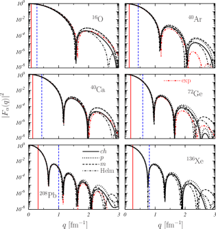
Figure 3: (Color on line) Nuclear form factors calculated with various density distributions. Full, dotted and dashed lines show the results obtained by using, respectively, the charge, proton and matter distributions obtained in our calculations. The red dashed-doubly-dotted lines are the form factors obtained by using the empirical charge distributions. The dashed-dotted lines indicate the form factors obtained within the Helm model. The vertical blue lines indicate the value of the momentum transfer corresponding to a nucleus kinetic energy of 100 keV.

Figure 4: Differences $\delta_{\alpha}(E_{R})$, as defined in Eq. (23), between the differential rates (1) calculated with our density distributions and those obtained with the Helm form factors. The values for the charge (solid lines), proton (dotted lines) and matter (dashed lines) distributions are shown. In each panel, the multiplication factors used to enlarge the y scale are indicated.

The form factors to be used in Eq. (6) to calculate the WIMP-nucleus cross section are shown in Fig. 3 where we have indicated, respectively, with full, dotted and dashed lines the results obtained by using the charge, proton and matter distributions obtained in our calculations. In the figure we also show with the red dashed- doubly-dotted lines the form factors obtained by using the empirical charge distributions. The dashed-dotted lines show the Helm form factors hel56 which are commonly used in the literature to calculate the WIMP-nucleus cross section. The Helm form factor is obtained by considering a charge density with a Gaussian surface distribution, and has a simple analytic expression

$$|F_{\rm Helm}(q)|^{2}\,=\,\left[\frac{3\,j_{1}(qR)}{qR}\right]^{2}\,\exp(-q^{2}s^{2})\,\,,$$ (19)

where $j_{1}$ is the first-order spherical Bessel function, and $R$ and $s$ are two parameters which are chosen to reproduce at best the experimental charge density distributions on all the nuclear chart. We used the parametrization suggested in Refs. lew96 ; che11

$$R^{2} = c^{2}\,-\,5s^{2}\,+\,18.65\,{\rm fm}^{2}\,\,\,,$$ (20)

$$c = \left(1.23\,A^{1/3}\,-\,0.6\,\right){\rm fm}\,\,\,,$$ (21)

$$s = 0.9\,{\rm fm}\,\,\,.$$ (22)

The differences between the various form factors increase with the value of $q$. This reflects the fact that, by increasing the resolution power, the probe is able to perceive the differences between the various densities. The form factors drop rather quickly with increasing value of $q$. The relevance of these differences in the calculation of the total event rate can be estimated by considering that, in the expression (5), the integration starts from the value of the threshold detection energy $E_{\rm th}$. As a reference example, in Fig. 3 we have indicated with vertical blue lines the values of the momentum transfer corresponding to a recoil energy, $E_{R}$, of 100 keV. This is a large value with respect to the performances of modern detectors. In this example, the form factors to the left hand side of the vertical lines do would not contribute to the total rate. This indicates that the largest values of the form factors are excluded, confirming an obvious consideration, the lower is the detection energy threshold, the higher is the rate of the detected events. More interesting is the comparison between the various nuclei. The heavier is the nucleus, the higher is the value of $q$ required to obtain a 100 keV recoil energy. For the two heavier nuclei ¹³⁶Xe and ²⁰⁸Pb, the lines appear after the first diffraction minimum, therefore, for these nuclei, the differences between the various densities can be more relevant.

We used our density distributions to calculate the differential, and total event rates, Eqs. (1) and (2). The values of the input parameters have been chosen coherently with what is used in the literature. If not stated otherwise, the results of the calculations we present in this paper have been obtained by assuming $\sigma_{\chi p}=$ 10^-42 cm² = 10^-16 fm², $\delta_{\chi}=0.3$ GeV/fm³, $v_{0}=0.001\,c$, $g_{np}=1$, $M_{\chi}=100$ GeV.

The first results we want to discuss are related to the differential rates of eq. (1). We show in Fig. 4 the differences

$$\delta_{\alpha}(E_{R})\,=\,\displaystyle\left[\frac{{\rm d}R(E_{R})}{{\rm d}E_{R}}\right]_{\alpha}\,-\,\left[\frac{{\rm d}R(E_{R})}{{\rm d}E_{R}}\right]_{\rm Helm}\,\,\,,$$ (23)

between the differential rates obtained with the distributions found in our calculations and those obtained by using the Helm form factors as a function of the recoil energy $E_{R}$. In these calculations we used a threshold detection energy of 10 eV only. Full, dotted and dashed lines show the differences obtained by using the charge ($\alpha=ch$), proton ($\alpha=p$) and matter ($\alpha=m$) densities, respectively.

A first observation is that these differences are rather small. The relative differences in the peaks of the figure are 5% at most. A second observation is that these differences increase with increasing mass number. The order of magnitude of these differences in ²⁰⁸Pb is 1000 times larger than that of ¹⁶O, 100 times larger than those of ⁴⁰Ca, ⁴⁰Ar and ⁷²Ge and, only, 10 times larger than that of ¹³⁶Xe. In all the nuclei we have considered, with the exception of ⁴⁰Ca, the smallest differences we found are those with the charge distributions. This could be expected since the parameters of the Helm form factors have been chosen to describe charge distributions. For the nuclei with $Z\neq N$ the results obtained with the proton distributions differ more than those obtained with the matter distributions. This is a direct consequence of what we have observed in Fig. 2.

Figure 5: Total rates, as given by Eq. (5), as a function of the threshold detection energy. The values found for the charge (solid lines), proton (dotted lines) and matter (dashed lines) distributions as well as those obtained with the Helm form factors (dashed-dotted lines) are shown. The values of the ¹⁶O nucleus have been multiplied by 10.

Figure 6: Relative differences, as defined by Eq. (24), between total rates calculated with matter distributions within our model and those obtained with the Helm form factors. The different lines show the results obtained by using different values of $M_{\chi}$.

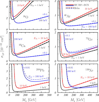
Figure 7: Upper limits of the WIMP-proton cross section, $\sigma_{\chi p}$, as a function of $M_{\chi}$, for the detection of a single event per day identified in an ideal detector of 100 tons, for $E_{\rm th}=1$, 10 and 100 keV. The solid lines show the results obtained by using our matter distributions obtained in HF or HF+BCS calculations, while the dashed-dotted lines indicate the results obtained by using the Helm form factors. The $E_{\rm th}=100$ keV results have been multiplied by 0.1 in case of ¹⁶O, ⁴⁰Ca, ⁴⁰Ar, ⁷²Ge nuclei, and by 0.01 for ¹³⁶Xe and ²⁰⁸Pb nuclei.

We show in Fig. 5 the total rates $R_{\alpha}(E_{\rm th})$ given by Eq. (5) as a function of the threshold energy. The different lines indicate the results obtained with the various densities. The behavior of the various lines is well understood. By increasing the value of the threshold energy, which means a lowering of the sensitivity of the detector, the number of the events becomes smaller. The comparison of the results obtained for the various nuclei indicates that at low values of $E_{\rm th}$ the heavier nuclei are more efficients in detecting events, because of the larger number of target nucleons inside the nucleus. We point out that, in the figure, the ¹⁶O results have been multiplied by a factor 10. On the other hand, the total rates drop more quickly in heavier nuclei than in lighter ones. At 40 keV the total rates expected in ²⁰⁸Pb are much smaller than those expected in the medium-heavy nuclei we have considered, ⁴⁰Ca, ⁴⁰Ar and ⁷²Ge.

The scale of Fig. 5 does not allow to appreciate the differences between the various results. For this reason, we have calculated the relative differences between the total rates obtained by using the matter distributions with respect to the results obtained with the Helm form factors

$$\Delta R_{m}(E_{\rm th})\,=\,\frac{R_{m}(E_{\rm th})\,-\,R_{\rm Helm}(E_{\rm th})}{R_{\rm Helm}(E_{\rm th})}\,\,\,.$$ (24)

These relative differences are shown in Fig. 6 as a function of $E_{\rm th}$. In this figure, in addition to the results related to total rates presented in Fig. 5, we show also results obtained by changing the WIMP mass $M_{\chi}$.

The value of the relative differences increases the heavier is the nucleus. We obtain a maximum value of 3% in ¹⁶O and 10-20% in ²⁰⁸Pb. The general enhancement with increasing $E_{\rm th}$ is more related to the lowering of the value in the denominator of Eq. (24) than to a real increase of the difference between the results obtained with matter and Helm distributions.

By comparing the results obtained with different values of $M_{\chi}$, we observe that $\Delta R$ increases with increasing mass. Since the minimum value of the momentum transfer for the detection is $q_{\rm min}=\sqrt{2\,E_{\rm th}\,M_{\chi}}$, if $M_{\chi}$ increases, also $q_{\rm min}$ increases. Therefore, a larger part of the form factors at low $q$, shown in Fig. 3, is excluded from the integral of Eq. (2), and the final result is more sensitive to the differences between various calculations, differences which appear at high $q$ values. In heavier nuclei, the increase of $E_{\rm th}$ moves the limit of this integration nearby the first minimum of the form factor, which is slightly displaced in the Helm model with respect to that obtained with the matter distribution.

To estimate the relevance of the differences in the use of the various form factors, we have calculated hypothetical values of the WIMP-proton cross section for which a rate of a single detected event per day is obtained in a 100 ton detector. For all the nuclei we have investigated, we show in Fig. 7 these limits, obtained for $E_{\rm th}=1$, 10 and 100 keV, as a function of the WIMP mass. The dashed-dotted curves correspond to the values found with the Helm form factors, while the solid lines indicate, respectively, those obtained by using our HF (for ¹⁶O, ⁴⁰Ca and ²⁰⁸Pb) and HF+BCS (for ⁴⁰Ar, ⁷²Ge and ¹³⁶Xe) matter distributions and HF+BCS (for ⁴⁰Ar, ⁷²Ge and ¹³⁶Xe). The $E_{\rm th}=100$ keV results have been multiplied by the factors indicated.

Obviously, the lower is $E_{\rm th}$, the lower is the line of the exclusion plot. The differences between our results and those obtained with the Helm form factors become larger with increasing target mass, with increasing $M_{\chi}$ values, and with increasing $E_{\rm th}$. These results show a minimum difference of 1.4% in the case of ¹⁶O for $E_{\rm th}=1$ keV, and a maximum one of 15% for ²⁰⁸Pb with $E_{\rm th}=100$ keV.

The results we have so far presented have been obtained by assuming the same coupling strength of the WIMP with protons and neutrons, i. e. $g_{np}=1$ in Eq. (6). We expect that, by releasing this assumption, as suggested, for example, in Ref. far11 , the requirement of a correct description of proton and neutron distributions becomes more important. For this reason, we have carried on calculations for different values of $g_{np}$. We have chosen values of $g_{np}$ producing extreme situations. The largest and smallest values we have considered, $\pm 2$, slightly exceed those indicated in far11 , values based on a compatibility analysis of the DAMA ber08 ; ber10 , CoGeNT aal11 and XENON100 apr11 data. The other values of $g_{np}$ have been chosen because of their physical meaning. The isospin conserving coupling, which has been our reference up to now, is obtained with $g_{np}=1$. The value $g_{np}=0$ selects only the WIMP-protons interaction. Finally, by using $g_{np}=-1$ we generate a cross section sensitive only to the differences between proton and neutron distributions.

Figure 8: Total rates, Eq. (5), calculated for different values of $g_{np}$, which are indicated in the insert of the ¹⁶O panel.

Figure 9: Relative differences between total rates calculated with our matter distributions and those obtained with the Helm form factor for $M_{\chi}=100$ GeV and for different values of $g_{np}$, indicated in the insert of the upper left panel.

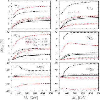
Figure 10: (Color on line) Relative differences between the limit values of $\sigma_{\chi p}$ calculated by using our matter distributions and those obtained with the Helm form factors. The results for $E_{\rm th}=1$ (full and red dotted lines), 10 (dashed-dotted and red dashed-double-dotted lines) and 100 keV (short-dashed and red long-dashed lines) are shown. Black full, dashed-dotted and short-dashed lines correspond to $g_{np}=1.0$, while red dotted, dashed-double-dotted and long-dashed lines correspond to the isotope violating hypothesis with $g_{np}=-2.0$.

The total rates calculated with these values of $g_{np}$, by using $M_{\chi}=100$ GeV, are shown in Fig. 8. In all the calculations the sequence of the various responses is similar. The lower lines are obtained with $g_{np}=-1$ the situation where the proton and neutron contribution cancel with each other. In the calculations where $F_{p}=F_{n}$, for example those which use the Helm form factors, the total rates for ¹⁶O and ⁴⁰Ca are exactly zero. Next we have the results with $g_{np}=0$ where the WIMP interacts only with the proton. We have then the results with $g_{np}=-2$ where the WIMP-neutron interaction dominates. In nuclei with $N=Z$ the total rates almost overlap with that obtained with $g_{np}=0$. For positive values of $g_{np}$ the total rates increase with increasing $g_{np}$. In Ref. far11 a value of about -1.5 has been suggested.

The aim of our work is to study the need of using accurate proton and neutron distributions to describe the WIMP-nucleus cross section. For this reason, we show in Fig. 9 the relative differences $\Delta R$, Eq. (24), obtained with the various values of $g_{np}$. In the two $N=Z$ nuclei, ¹⁶O and ⁴⁰Ca, the results with $g_{np}=-1$ are not indicated since in this case $R_{\rm Helm}$ is zero with the obvious consequences in the calculation of $\Delta R$.

The behavior of the various lines has different characteristics for the $N=Z$ nuclei and for the other ones. In the former cases the smaller differences appear for $g_{np}=0$ and the largest ones for $g_{np}=-2$. The relative differences can reach values around the 20% in heavy nuclei.

We have evaluated the consequences of these differences by calculating limits as those shown in Fig. 7 with different values of $g_{np}$. We show in Fig. 10 the relative differences $\Delta\sigma_{\chi p}$ between the limits of the WIMP-proton cross section calculated with our matter distributions and those obtained with the Helm form factors. The results for $E_{\rm th}=1,10,100$ keV are shown. The black (full, dashed-dotted and short-dashed) lines show the relative differences of our reference calculations done with $g_{np}=1$, i.e. those obtained from the results of Fig. 7. The red (dotted, dashed-doubly-dotted and log-dashed) lines indicate the differences obtained with $g_{np}=-2$, a value comparable with that suggested in Ref. far11 . In all the cases the largest differences have been obtained for a threshold energy of 100 keV. As it has been previously discussed, the differences are enhanced with increasing $E_{\rm th}$. We do not identify common trends in this figure. Sometime the $g_{np}=-2$ results show the largest differences, in other cases the largest differences are produced by $g_{np}=1$. We observe that in ⁴⁰Ar, ⁷²Ge and ¹³⁶Xe these values can reach the 20%.

IV Conclusions

In this work, we have studied the validity of the approximation commonly done in the literature consisting in considering the nuclear charge density instead than the matter density in the calculation of the WIMP-nucleus cross sections. While charge distributions are experimentally known for various nuclei with high accuracy dej87 , the matter distributions are essentially unknown. For this reason, we propose to use the point-like matter distributions obtained in mean-field calculations of HF type. We present here the results obtained with a specific implementation of the HF calculations, involving an effective finite range interaction of Gogny type dec80 . Our experience co12a indicates that these results are general and more related to the mean-field description of the nucleus rather than to its specific implementation.

We have shown that our model describes well the experimental charge distributions, and we have assumed that it is also able to properly describe the matter distributions. We have compared the form factors calculated with our matter distributions with the Helm form factors commonly adopted in the literature. The differences between the factors calculated by using different distributions show up at high values of the momentum transfer, usually after the first diffraction minimum. The relevance of these differences is strictly related to the value of the detection threshold energy $E_{\rm th}$, and decreases with it.

We have calculated differential, total rates and upper detections limits. In this last case, we found that the differences between our results and those obtained with the Helm form factor become larger with increasing target mass, with increasing $M_{\chi}$ values, and with increasing $E_{\rm th}$. We found a maximum relative difference of about 15% for ²⁰⁸Pb with $E_{\rm th}=100$ keV.

The requirement of using matter instead than charge distributions in the calculation of the WIMP-nucleus cross section becomes more important when the assumption of isospin conserving WIMP-nucleon interaction is released. In this case, the proton and neutron distributions are mixed with different weights, therefore an accurate description of the two distributions is mandatory. Also in this case, the value of $E_{\rm th}$ is the parameter which dominates the value of the uncertainty, however, the use of mixing values close to those suggested in the literature increases the difference with respect the results obtained with the Helm model. In specific situations the relative differences can reach the value of 20%.

In the estimation of the total event rate related to the WIMPs detection, the values of many input quantities are unknown, and strong assumptions are done on them. On the other hand, the nuclear physics part of the process is well understood, and we propose to use the modern nuclear structure results to improve its description.

Appendix: Fourier-Bessel coefficients of density distributions

In this appendix we show the values of the Fourier-Bessel coefficients which allow the reconstruction of our proton and neutron density distributions for the nuclei we have considered. These distributions can be obtained by the expression

$$\rho(r)\,=\,\sum_{\mu=1}^{M}A_{\mu}\,\frac{\sin(q_{\mu}r)}{q_{\mu}r}\,\,\,,$$ (25)

where the $q_{\mu}$ are defined as

$$q_{\mu}=\mu\frac{\pi}{R}\,\,\,,$$

with $R$ the maximum value of the radius where the density is supposed to be different from zero. The density distributions obtained with the coefficients given in Tables 3 and 4, have the usual nuclear physics normalizations, i. e. the integrals of Eq. (8) are normalized to the number of protons or neutrons.

		16O			40Ca			208Pb
$\mu$		proton	neutron		proton	neutron		proton	neutron
1		2.89514E-02	2.90605E-02		6.17474E-02	6.23662E-02		7.69622E-02	1.16349E-01
2		5.44734E-02	5.53342E-02		5.75764E-02	6.08146E-02		1.87236E-02	2.73910E-02
3		2.37463E-02	2.50485E-02		-2.94985E-02	-2.82238E-02		-6.54988E-02	-8.28045E-02
4		-1.51728E-02	-1.46814E-02		-1.93097E-02	-2.10479E-02		3.20906E-02	4.81394E-02
5		-1.94164E-02	-1.99175E-02		1.87819E-02	1.85152E-02		1.42479E-02	1.17763E-02
6		-5.40039E-03	-6.14889E-03		9.02298E-03	9.93418E-03		-2.81145E-02	-2.99372E-02
7		1.85720E-03	1.34614E-03		-1.89926E-03	-2.77723E-03		1.43845E-02	1.88786E-02
8		6.24424E-04	3.75985E-04		1.40503E-03	-1.48915E-03		1.53527E-02	-6.90422E-03
9		-1.18242E-03	-1.29026E-03		2.91761E-03	-1.02014E-03		3.00274E-03	-2.34458E-02
10		-9.50609E-04	-9.80391E-04		1.34965E-03	-2.77186E-03		3.76239E-03	-1.08603E-03
11		-1.71403E-04	-1.66395E-04		1.77650E-03	-2.38989E-03		-4.27147E-03	5.77452E-03
12		4.61957E-05	6.54090E-05		1.68542E-03	-1.69061E-03		-3.33174E-03	2.14901E-03
13		-1.93572E-05	-9.66199E-06		1.13150E-03	-8.69682E-04		3.06557E-03	-8.57191E-04
14		-7.29176E-05	-6.72835E-05		2.12233E-04	-4.41138E-04		1.80972E-03	-3.12159E-03
15		-	-		2.61156E-04	4.04638E-05		-3.10532E-04	4.46753E-04
R [fm]		7.0	7.0		7.0	7.0		10.0	10.0

Table 3: Fourier-Bessel coefficients $A_{\mu}$ and radii $R$, see Eq. (25), for the proton and neutron densities obtained in the HF calculations.

		40Ar			72Ge			136Xe
$\mu$		proton	neutron		proton	neutron		proton	neutron
1		3.09708E-02	3.76246E-02		4.98732E-02	6.18996E-02		4.64213E-02	6.96034E-02
2		5.88325E-02	7.02530E-02		6.19545E-02	7.60695E-02		5.66577E-02	8.15343E-02
3		2.10665E-02	2.43967E-02		-1.96985E-02	-1.88170E-02		-2.89511E-02	-3.93097E-02
4		-2.71647E-02	-3.07229E-02		-3.69138E-02	-3.41701E-02		-4.44567E-02	-5.02359E-02
5		-2.58345E-02	-2.67849E-02		1.29234E-02	1.68135E-02		2.16418E-02	3.33255E-02
6		1.35027E-03	5.39599E-03		2.33454E-02	1.51003E-02		2.99702E-02	2.78136E-02
7		1.14853E-02	1.73114E-02		3.16112E-03	-1.37351E-02		-1.22571E-02	-2.05113E-02
8		3.83701E-03	9.32738E-03		-8.94086E-04	-1.58768E-02		-2.07746E-02	-7.97235E-03
9		-2.49991E-03	2.11831E-03		3.68467E-03	-5.21935E-03		-4.58139E-03	2.24455E-02
10		-2.09091E-03	1.01436E-03		2.56986E-03	-1.03807E-03		-8.95531E-04	1.91808E-02
11		-1.66806E-04	1.16466E-03		1.12422E-04	-7.28180E-04		-3.60592E-03	5.18993E-03
12		3.19675E-04	4.98071E-04		-2.13356E-04	-3.48872E-04		-1.72562E-03	1.49995E-03
13		8.86515E-05	-8.27115E-05		7.99035E-05	4.73510E-06		4.85598E-04	1.63508E-03
14		-	-		7.52024E-05	1.45816E-05		4.04238E-04	6.51292E-04
15		-	-		4.16595E-05	1.51430E-05		-	-
R [fm]		9.0	9.0		9.0	9.0		11.0	11.0

Table 4: Fourier-Bessel coefficients $A_{\mu}$ and radii $R$, see Eq. (25), for the proton and neutron densities obtained in the HF + BCS calculations.

References

- (1) R. Bernabei et al., New results from DAMA/LIBRA, Eur. Phys. Jour. C 67 (2010) 39.
- (2) C. E. Aalseth et al., Results from a search for light-mass dark matter with a p-type point contact germanium detector, Phys. Rev. Lett. 106 (2011) 131301.
- (3) Z. Ahmed et al., Results from a low-energy analysis of the CDMS II germanium data,Phys. Rev. Lett. 106 (2011) 131302.
- (4) E. Aprile et al., Dark matter results from 100 live days of XENON100 data, Phys. Rev. Lett. 107 (2011) 131302.
- (5) E. Armengaud et al. Final results of the EDELWEISS-II WIMP search using a 4-kg array of cryogenic germanium detectors with interleaved electrodes, Phys. Lett. B 702 (2011) 329.
- (6) J. Engel, S. Pittel and P. Vogel, Nuclear physics of dark matter detection, em Int. Jour. Mod. Phys. E 1 (1992) 1.
- (7) R. Helm, Inelastic and elastic scattering of 187-MeV electrons from selected even-even nuclei, Phys. Rev. 104 (1956) 1466.
- (8) G. Dūda, A. Kemper and P. Gondolo, Model-independent form factors for spin-independent neutralino-nucleon scattering from elastic electron scattering data, JCAP 4 (2007) 12.
- (9) C. W. de Jager and C. de Vries, Nuclear charge-density-distributions parameters, At. Data Nucl. Data Tables 36 (1987) 495.
- (10) Y. Z. Chen, Y. A. Luo, L. Li, H. Shen and X. Q. Li, Determining Nuclear Form factor for Detection of Dark Matter in Relativistic Mean Field Theory , Commun. Theor. Phys. 55 (2011) 1059.
- (11) J. Dechargè, D. Gogny, Hartree-Fock-Bogolyubov calculations with the D1 effective interaction on spherical nuclei, Phys. Rev. C 21 (1980) 1568.
- (12) G. Co’ et al. Mean-field calculations of the ground states of exotic nuclei, Phys. Rev. C 85 (2012) 024322.
- (13) P. Ring and P. Schuck, The nuclear many-body problem, Springer, Berlin, 1980.
- (14) J. F. Berger, M. Girod and D. Gogny, Time-dependent quantum collective dynamics applied to nuclear fission, Comp. Phys. Commun. 63 (1991) 365.
- (15) S. Goriely, S. Hilaire, M. Girod and S. Péru, First Gogny-Hartree-Fock-Bogoliubov nuclear mass model, Phys. Rev. Lett. 102 (2009) 242501.
- (16) D. Acosta-Kane et al., Discovery of underground argon with low level of radioactive 39Ar and possible applications to WIMP dark matter detectors, Nucl. Inst. Meth. A 587 (2008) 46.
- (17) S. Boffi, C. Giusti, F. D. Pacati and M. Radici, Electromagnetic response of atomic nuclei, Clarendon, Oxford, 1996.
- (18) G. Hoeler et al. Analysis of electromagnetic nucleon form factors, Nucl. Phys. B 114 (1976) 505.
- (19) J. M. Cavedon et al., Is the Shell-Model Concept Relevant for the Nuclear Interior?, Phys. Rev. Lett. 49 (1982) 978.
- (20) G. Co’ and J. Speth, Charge distribution differences in heavy mass nuclei, Z. Phys. A 326 (1987) 361.
- (21) M. Anguiano and G. Co’, Correlations and charge distributions of medium heavy nuclei, Jour. Phys. G 27 (2001) 2109.
- (22) J. D. Lewin and P. F. Smith, Review of mathematics, numerical factors, and corrections for dark matter experiments based on elastic nuclear recoil, Astroparticle Phys. 6 (1996) 87.
- (23) M. Farina, D. Pappadopulo, A. Strumia, T. Volansky, Can CoGeNT and DAMA modulations be due to Dark Matter?, JCAP 11 (2011) 10.
- (24) R. Bernabei et al., First results from DAMA/LIBRA and the combined results with DAMA/NaI, Eur. Phys. Jour. C 56 (2008) 333.