Unconditionally optimal error estimates of a Crank–Nicolson Galerkin method for the
nonlinear thermistor equations

Abstract

This paper focuses on unconditionally optimal error analysis of an uncoupled and linearized Crank–Nicolson Galerkin finite element method for the time-dependent nonlinear thermistor equations in $d$-dimensional space, $d=2,3$. We split the error function into two parts, one from the spatial discretization and one from the temporal discretization, by introducing a corresponding time-discrete (elliptic) system. We present a rigorous analysis for the regularity of the solution of the time-discrete system and error estimates of the time discretization. With these estimates and the proved regularity, optimal error estimates of the fully discrete Crank–Nicolson Galerkin method are obtained unconditionally. Numerical results confirm our analysis and show the efficiency of the method.

Key words: Unconditional optimal error analysis, linearized Crank–Nicolson scheme, Galerkin FEM, nonlinear thermistor equation

1 Introduction

We consider the time-dependent nonlinear thermistor system

$$\frac{\partial u}{\partial t}-\Delta u=\sigma(u)|\nabla\phi|^{2},$$ (1.1)

$$-\nabla\cdot(\sigma(u)\nabla\phi)=0,$$ (1.2)

for $x\in\Omega$ and $t\in[0,T]$, where $\Omega$ is a bounded domain in $\mathbb{R}^{d}$, $d=2,3$. The initial and boundary conditions are given by

$$\begin{array}[]{ll}u(x,t)=0,\quad\phi(x,t)=g(x,t){}{}&\mbox{for}~{}~{}x\in\partial\Omega,~{}~{}t\in[0,T],\\[3.0pt] u(x,0)=u_{0}(x){}{}&\mbox{for}~{}~{}x\in\Omega.\end{array}$$ (1.5)

The nonlinear system above describes the model of electric heating of a conducting body, where $u$ is the temperature, $\phi$ is the electric potential, and $\sigma$ is the temperature-dependent electric conductivity. Following the previous works [14, 38], we assume that $\sigma\in W^{1,\infty}(\mathbb{R})$ and

$$\sigma_{1}\leq\sigma(s)\leq\sigma_{2},$$ (1.6)

for some positive constants $\sigma_{1}$ and $\sigma_{2}$.

Theoretical analysis for the time-dependent thermistor equations was done by several authors [3, 5, 10, 36, 37]. Among these works, Yuan and Liu [37] proved the existence and uniqueness of a $C^{\alpha}$ solution in three-dimensional space. Based on their result, further regularity can be derived with suitable assumptions on the initial and boundary conditions. Numerical methods and analysis for the thermistor system can be found in [2, 4, 14, 35, 38, 39]. For the system in two-dimensional space, the optimal $L^{2}$ error estimate of a mixed finite element method with a linearized semi-implicit Euler scheme was obtained in [38] under a weak time-step condition. Error analysis for the three-dimensional model was given in [14], in which a linearized semi-implicit Euler scheme with a linear Galerkin FEM was used. An optimal $L^{2}$-error estimate was obtained under the condition $\tau=O(h^{1/2})$. A more general time discretization with higher-order finite element approximations was studied in [2]. An optimal $L^{2}$-norm error estimate was given under the conditions $\tau=O(h^{3/2p})$ and $r\geq 2$, where $p$ is the order of the time discretization and $r$ is the degree of piecewise polynomials of the finite element space.

Clearly, there are several different time discretizations for nonlinear parabolic systems, explicit, semi-explicit (or semi-implicit) and implicit. The most popular and widely-used approach is linearized (semi)-implicit scheme. At each time step, the scheme only requires the solution of a linear system. However, time-step condition is always a key issue for such a scheme. To study the error estimate of linearized (semi)-implicit schemes, the boundedness of the numerical solution (or error function) in $L^{\infty}$ norm or a stronger norm is often required. If a priori estimate for numerical solution in such a norm cannot be provided, one may employ the mathematical induction with an inverse inequality to bound the numerical solution, such as, by

$$\|U_{h}^{n}-R_{h}u^{n}\|_{L^{\infty}}\leq Ch^{-d/2}\|U_{h}^{n}-R_{h}u^{n}\|_{L^{2}}\leq Ch^{-d/2}(\tau^{m}+h^{r+1}),$$ (1.7)

where $U^{n}_{h}$ is the finite element solution, $u^{n}$ is the exact solution and $R_{h}$ is certain projection operator. The above approach, however, requires a time-step condition $\tau=O(h^{d/(2m)})$. This approach has been widely used in the error analysis of many different nonlinear parabolic PDEs, $e.g.$, see [16, 18, 23] for Navier-Stokes equations, [2, 14, 38] for nonlinear thermistor problems, [15, 28, 31] for porous media flows, [8, 32] for viscoelastic fluid flow, [24] for KdV equations, [9, 25] for the Ginzburg-Landau equations, [6, 30] for nonlinear Schrödinger equations and [12, 34] for some other equations. In all these works, error estimates were established under certain time step restrictions. The time-step restrictions arising from theoretical analysis may result in the use of a very small time step and extremely time-consuming in practical computations. However, we believe that such time-step conditions may not be necessary for most cases. A new approach was introduced in our recent works [20, 21], also see [22], in which the error estimates of a linearized backward Euler Galerkin methods for a porous media flow and the thermistor system were obtained, respectively, under the condition of $h$ and $\tau$ being smaller than a positive constant. In this paper, we propose an uncoupled and linearized Crank–Nicolson Galerkin finite element method for the nonlinear thermistor system and present optimal error estimates in both $L^{2}$ and $H^{1}$ norms without any stepsize restrictions. In this method, the standard Crank–Nicolson scheme is applied for the linear term in the temperature equation and an extrapolation approximation is used for the nonlinear electric conductivity. At each time step, one only needs to solve two uncoupled linear systems. The main idea of our aprooach is to split the error function into two parts, the spatially discrete error and the temporally discrete error, by introducing a corresponding time-discrete (elliptic) system. The former arises from the Galerkin FEM discretization for the time-discrete equations and depends only upon the spatial mesh size $h$ (independent of the time-step size $\tau$). If a suitable regularity of the solution to the time-discrete equations has been proved, the numerical solution can be bounded by

$$\|U_{h}^{n}-R_{h}U^{n}\|_{L^{\infty}}\leq Ch^{-d/2}\|U_{h}^{n}-R_{h}U^{n}\|_{L^{2}}\leq Ch^{-d/2}h^{r+1}$$ (1.8)

without any time-step condition, where $U^{n}$ is the solution of the time-discrete equations. More important is that our approach is applicable for more general nonlinear parabolic PDEs and many other time discretizations to obtain unconditional convergence and optimal error estimates.

The rest of the paper is organized as follows. In Section 2, we present the uncoupled and linearized Crank–Nicolson scheme with a linear Galerkin finite element approximation in the spatial direction and state our main results. After introducing the corresponding time-discrete system, we provide in Section 3 a priori estimates and optimal error estimates for the time-discrete solution, which imply the suitable regularity of the time-discrete solution. With the regularity obtained, in Section 4 we present optimal error estimates of the fully discrete Galerkin finite element solution in both the $L^{2}$ norm and the $H^{1}$ norm without any time-step conditions. Numerical results are presented in Section 5 to confirm our theoretical analysis.

2 The main result

Let $\Omega$ be a bounded, smooth and convex domain in $\mathbb{R}^{d}$ ($d=2,3$). Let $\pi_{h}$ be a regular division of $\Omega$ into triangles $T_{j}$, $j=1,\cdots,M$ in $\mathbb{R}^{2}$ or tetrahedra in $\mathbb{R}^{3}$, and denote by $h=\max_{1\leq j\leq M}\{\mbox{diam}\,T_{j}\}$ the mesh size. For a triangle (or tetrahedra) $T_{j}$ at the boundary, we define $\tilde{T}_{j}$ to be a triangle with one curved side (or a tetrahedra with one curved face in $\mathbb{R}^{3}$) with the same vertices as $T_{j}$, and set $D_{j}=\tilde{T}_{j}\backslash T_{j}$. For an interior triangle, we set $\tilde{T}_{j}=T_{j}$ and $D_{j}=\emptyset$. For a given triangular (or tetrahedral) division of $\Omega$, we define the finite element spaces [29]:

$$V_{h}=\{v_{h}\in C(\overline{\Omega}):v_{h}|_{T_{j}}\mbox{~{}is~{}linear~{}at~{}each~{}element~{}and~{}}v_{h}=0~{}\mbox{on}~{}D_{j}\},$$

$$S_{h}=\{v_{h}\in C(\overline{\Omega}):v_{h}|_{\widetilde{T}_{j}}\mbox{~{}is~{}linear~{}at~{}each~{}element}\}.$$

It follows that $V_{h}$ is a subspace of $H^{1}_{0}(\Omega)$ and $S_{h}$ is a subspace of $H^{1}(\Omega)$. For any function $v\in S_{h}$, we define $\Lambda_{h}v$ to be a function satisfying $\Lambda_{h}v=0$ on $D_{j}$ and $\Lambda_{h}v=v$ on $T_{j}$. We further define $\widetilde{\Pi}_{h}:C_{0}(\overline{\Omega})\rightarrow S_{h}$ to be the Lagrangian interpolation operator and set $\Pi_{h}=\Lambda_{h}\widetilde{\Pi}_{h}$. Clearly, $\Pi_{h}$ is a projection operator from $C_{0}(\overline{\Omega})$ onto $V_{h}$.

Let $0=t_{0}<t_{1}<\cdots<t_{N}=T$ be a uniform partition of the time interval $[0,T]$ with $t_{n}=n\tau$ and let

$$u^{n}=u(x,t_{n}),\quad\phi^{n}=\phi(x,t_{n})\,\qquad\mbox{for}\quad n=0,1,\cdots,N.$$ (2.1)

For any sequence of functions $\{f^{n}\}_{n=0}^{N}$, we define

$$D_{\tau}f^{n+1}=\frac{f^{n+1}-f^{n}}{\tau},\qquad\widehat{f}^{n+1/2}=(3f^{n}-f^{n-1})/2,$$ (2.2)

$$\bar{f}^{n+1/2}=\frac{1}{2}(f^{n}+f^{n+1}),$$ (2.3)

for $n=1,2,\cdots,N-1$.

For the simplicity of notations, we denote by $C$ a generic positive constant and by $\epsilon$ a generic small positive constant, which depend solely upon the physical parameters of the problem and independent of $\tau$, $h$ and $n$. We assume that $g(\cdot,t)\in H^{1}(\Omega)$ is given for each fixed $t\geq 0$.

We propose an uncoupled and linearized Crank–Nicolson Galerkin finite element method to solve the system (1.1)-(1.5), which seeks $U^{n+1}_{h}\in V_{h}$ and $\Phi^{n+1/2}_{h}\in g^{n-1/2}+V_{h}$, $n=0,1,\cdots,N-1$, such that

$$\Big{(}\sigma(\widehat{U}_{h}^{n+1/2})\nabla\Phi_{h}^{n+1/2},\nabla\varphi\Big{)}=0,\quad\forall~{}\varphi\in V_{h},$$ (2.4)

$$\Big{(}D_{\tau}U^{n+1}_{h},v\Big{)}+\Big{(}\nabla\overline{U}_{h}^{n+1/2},\nabla v\Big{)}=\Big{(}\sigma(\widehat{U}_{h}^{n+1/2})|\nabla\Phi_{h}^{n+1/2}|^{2},v\Big{)},\quad\forall~{}v\in V_{h}$$ (2.5)

where a standard extrapolation [13] is used to approximate the nonlinear electric conductivity for $n>0$.

At the initial time steps, we choose $U^{0}_{h}=\Pi_{h}u_{0}$ and let $\Phi^{0}_{h}$ be the Galerkin solution to the potential equation

$$\Big{(}\sigma(u_{0})\nabla\Phi_{h}^{0},\nabla\varphi\Big{)}=0,\quad\forall~{}\varphi\in V_{h}.$$ (2.6)

and $\widehat{U}_{h}^{1/2}$ can be calculated either by a semi-implict Euler scheme

$$\Big{(}\frac{\widehat{U}^{1/2}_{h}-u^{0}}{\tau/2},v\Big{)}+\Big{(}\nabla\widehat{U}_{h}^{1/2},\nabla v\Big{)}=\Big{(}\sigma(u_{0})|\nabla\Phi_{h}^{0}|^{2},v\Big{)},\quad\forall~{}v\in V_{h}$$ (2.7)

or by an explicit Euler scheme

$$\Big{(}\frac{\widehat{U}^{1/2}_{h}-u^{0}}{\tau/2},v\Big{)}+\Big{(}\nabla u_{0},\nabla v\Big{)}=\Big{(}\sigma(u_{0})|\nabla\Phi_{h}^{0}|^{2},v\Big{)},\quad\forall~{}v\in V_{h}$$ (2.8)

By the classical finite element theory for elliptic equations and for interpolation, we have

$$\|U^{0}_{h}-u_{0}\|_{L^{2}}+\|\Phi_{h}^{0}-\phi^{0}\|_{L^{12/5}}\leq Ch^{2}.$$ (2.9)

Here we assume that the solution of the initial/boundary value problem (1.1)-(1.5) exists and satisfies

$$\|u_{0}\|_{H^{2}}+\|u\|_{L^{\infty}((0,T);H^{2})}+\|u_{t}\|_{L^{\infty}((0,T);H^{2})}$$

$$+\|u_{tt}\|_{L^{\infty}((0,T);H^{1})}+\|u_{tt}\|_{L^{2}((0,T);H^{2})}+\|u_{ttt}\|_{L^{2}((0,T);L^{2})}\leq C,$$ (2.10)

and

$$\|\phi\|_{L^{\infty}((0,T);W^{2,12/5})}+\|\phi_{t}\|_{L^{\infty}((0,T);W^{1,6})}+\|\nabla\phi\|_{L^{\infty}((0,T);L^{\infty})}$$

$$+\|g\|_{L^{\infty}((0,T);W^{2,12/5})}+\|\nabla g\|_{L^{\infty}((0,T);L^{\infty})}\leq C.$$ (2.11)

The emphasis of this paper is on the unconditionally optimal error analysis. The above regularity assumptions may possibly be weakened for the analysis below. We present our main result in the following theorem. The proof will be given in Sections 3-4.

Theorem 2.1

Suppose that the system (1.1)-(1.2) with the initial and boundary conditions (1.5) has a unique solution $(u,\phi)$ satisfying (2)-(2). Then the finite element system (2.4)-(2.7) admits a unique solution $(U^{n}_{h},\,\Phi^{n-1/2}_{h})$, $n=1,\cdots,N$, such that

$$\max_{1\leq n\leq N}\|U^{n}_{h}-u(\cdot,t_{n})\|_{L^{2}}+\max_{1\leq n\leq N}\|\Phi^{n-1/2}_{h}-\phi(\cdot,t_{n-1/2})\|_{L^{12/5}}\leq C(\tau^{2}+h^{2}),$$ (2.12)

$$\max_{1\leq n\leq N}\|U^{n}_{h}-u(\cdot,t_{n})\|_{H^{1}}+\max_{1\leq n\leq N}\|\Phi^{n-1/2}_{h}-\phi(\cdot,t_{n-1/2})\|_{W^{1,12/5}}\leq C(\tau^{2}+h).$$ (2.13)

To prove Theorem 2.1, we introduce a time-discrete system of equations:

$$\nabla\cdot\big{(}\sigma(\widehat{U}^{n+1/2})\nabla\Phi^{n+1/2}\big{)}=0,\qquad\qquad\qquad\qquad~{}~{}~{}\mbox{for $n=0,1,\cdots$}$$ (2.14)

$$D_{\tau}U^{n+1}-\Delta\overline{U}^{n+1/2}=\sigma(\widehat{U}^{n+1/2})|\nabla\Phi^{n+1/2}|^{2},\qquad~{}\mbox{for $n=0,1,\cdots$}$$ (2.15)

subject to the boundary/initial conditions

$$\begin{array}[]{ll}U^{n}(x)=0,\quad\Phi^{n+1/2}(x)=g(x,t_{n+1/2}){}{}&\mbox{for}~{}~{}x\in\partial\Omega,~{}~{}1\leq n\leq N,\\[3.0pt] U^{0}(x)=u_{0}(x){}&\mbox{for}~{}~{}x\in\Omega\\[5.0pt] \displaystyle\frac{\widehat{U}^{1/2}-U^{0}}{\tau/2}-\Delta\widehat{U}^{1/2}=\sigma(u_{0})|\nabla\phi^{0}|^{2}{}&\mbox{for}~{}~{}x\in\Omega\,,\\[5.0pt] \widehat{U}^{1/2}=0,{}{}&\mbox{for}~{}~{}x\in\partial\Omega,\end{array}$$ (2.20)

where $\phi^{0}$ is the solution to the elliptic equation

$$\left\{\begin{array}[]{ll}\nabla\cdot(\sigma(u_{0})\nabla\phi^{0})=0\quad\mbox{in}~{}~{}\Omega,\\[5.0pt] \phi^{0}(x)=g(x,0)\quad\mbox{for}~{}~{}x\in\partial\Omega.\end{array}\right.$$ (2.23)

With the solution of the time-discrete system $(U^{n},\Phi^{n-1/2})$, we have the following error splitting:

$$\|U^{n}_{h}-u^{n}\|\leq\|e^{n}\|+\|U^{n}-U_{h}^{n}\|$$

$$\|\Phi_{h}^{n-1/2}-\phi^{n-1/2}\|\leq\|\eta^{n-1/2}\|+\|\Phi^{n-1/2}-\Phi_{h}^{n-1/2}\|$$

where

$$e^{n}=U^{n}-u^{n},\qquad\eta^{n-1/2}=\Phi^{n-1/2}-\phi^{n-1/2}\,.$$

Note that the fully discrete system (2.4)-(2.5) can be viewed as the spatial discretization of the elliptic system (2.14)-(2.15). The key issue is to prove the regularity of the solution to the time-discrete equations (2.14)-(2.15) required in the error estimates of the Galerkin finite element method. We present the estimates of the error functions $(e^{n},\eta^{n-1/2})$ and $(U^{n}-U_{h}^{n},\,\Phi^{n-1/2}-\Phi_{h}^{n-1/2})$ in Section 3 and Section 4, respectively.

Moreover, the error estimates given in the above theorem for $\Phi$ are defined in the time level $t_{n-1/2}$. To get the solution at the time level $t_{n}$, we define

$$\Phi_{h}^{n}:=\frac{1}{2}(\Phi_{h}^{n+1/2}+\Phi_{h}^{n-1/2})\,.$$

By the above theorem, we see that

$$\max_{1\leq n\leq N}\|\Phi^{n}_{h}-\phi(\cdot,t_{n})\|_{L^{12/5}}\leq C(\tau^{2}+h^{2}),$$ (2.24)

$$\max_{1\leq n\leq N}\|\Phi^{n}_{h}-\phi(\cdot,t_{n})\|_{W^{1,12/5}}\leq C(\tau^{2}+h).$$ (2.25)

The following lemma can be proved by noting the definition (2.3) and using a triangular inequality.

Lemma 2.1

Let $\{v^{n}\}_{n=0}^{N}$ be a sequence of functions on $\Omega$. Then for any norm $\|\cdot\|$,

$$\tau\|v^{n}\|\leq 2\tau\sum_{m=1}^{n}\|\overline{v}^{m-1/2}\|+\tau\|v^{0}\|\leq 2\sqrt{T}\sqrt{\sum_{m=1}^{n}\tau\|\overline{v}^{m-1/2}\|^{2}}+\tau\|v^{0}\|\,.$$ (2.26)

3 Temporal error analysis

In this section, we prove the existence and uniqueness of the solution of the time-discrete system (2.14)-(2.20) and establish error bounds for $(e^{n},\eta^{n-1/2})$.

Theorem 3.1

Suppose that the system (1.1)-(1.5) has a unique solution $(u,\phi)$ satisfying (2)-(2). Then the time-discrete system (2.14)-(2.20) admits a unique solution $(U^{n},\Phi^{n-1/2})$ such that

$$\max_{1\leq n\leq N}\|U^{n}\|_{H^{2}}+\max_{1\leq n\leq N}\|D_{\tau}U^{n}\|_{H^{2}}+\|D_{\tau}\widehat{U}^{1/2}\|_{H^{2}}\leq C,$$ (3.1)

$$\max_{1\leq n\leq N}\|\Phi^{n-1/2}\|_{W^{2,12/5}}+\max_{1\leq n\leq N}\|\nabla\Phi^{n-1/2}\|_{L^{p}}\leq C,\quad\forall~{}1\leq p<\infty,$$ (3.2)

and

$$\begin{array}[]{ll}&\displaystyle\max_{1\leq n\leq N}\|e^{n}\|_{H^{1}}+\max_{1\leq n\leq N}\|\eta^{n-1/2}\|_{W^{1,12/5}}\leq C\tau^{2}.\end{array}$$ (3.4)

Proof    The existence and uniqueness of solution to the linear partial differential equations (2.14)-(2.20) is obvious. In the following, we only prove the estimates (3.1)-(3.4).

Since $U^{0}=u^{0}$, the error functions $e^{n+1}$ and $\eta^{n+1/2}$, $0\leq n\leq N-1$, satisfy

$$-\nabla\cdot\big{[}\sigma(\widehat{U}^{n+1/2})\nabla\eta^{n+1/2}\big{]}=\nabla\cdot\big{[}(\sigma(\widehat{u}^{n+1/2})-\sigma(\widehat{U}^{n+1/2}))\nabla\phi^{n+1/2}\big{]}+\nabla\cdot R_{\phi}^{n+1/2},$$ (3.5)

$$D_{\tau}e^{n+1}-\Delta\overline{e}^{n+1/2}=(\sigma(\widehat{U}^{n+1/2})-\sigma(\widehat{u}^{n+1/2}))|\nabla\phi^{n+1/2}|^{2}$$ (3.6)

$$~{}~{}~{}~{}~{}~{}~{}~{}~{}~{}~{}~{}~{}~{}~{}~{}~{}~{}~{}~{}~{}~{}~{}~{}~{}+\sigma(\widehat{U}^{n+1/2})(\nabla\phi^{n+1/2}+\nabla\Phi^{n+1/2})\cdot\nabla\eta^{n+1/2}+R_{u}^{n+1},$$

and

$$\frac{2}{\tau}\widehat{e}^{1/2}-\Delta\widehat{e}^{1/2}=R_{u}^{1/2},$$ (3.7)

where

$$R_{u}^{1/2}=u_{t}|_{t=0}-\frac{u^{1/2}-u^{0}}{\tau/2}+\sigma(u^{0})|\nabla\phi^{0}|^{2}-\sigma(u^{1/2})|\nabla\phi^{1/2}|^{2}\,$$

$$R_{u}^{n+1}=\frac{\partial u}{\partial t}\Big{|}_{t=t_{n+1/2}}\!\!\!\!\!-D_{\tau}u^{n+1}+\Delta(\overline{u}^{n+1/2}-u^{n+1/2})+(\sigma(u^{n+1/2})-\sigma(\widehat{u}^{n+1/2}))|\nabla\phi^{n+1/2}|^{2}\,,$$

$$R_{\phi}^{n+1/2}=(\sigma(u^{n+1/2})-\sigma(\widehat{u}^{n+1/2}))\nabla\phi^{n+1/2}$$

are the truncation errors. With the regularity given in (2)-(2), we have the following estimates for the truncation errors:

$$\max\limits_{0\leq n\leq N-1}\|R_{\phi}^{n+1/2}\|_{L^{6}}+\left(\sum_{n=0}^{N-1}\tau\|R_{u}^{n+1}\|_{L^{2}}^{2}\right)^{\frac{1}{2}}+\tau\|R^{1/2}_{u}\|_{L^{6}}\leq C\tau^{2}.$$ (3.8)

To prove (3.1)-(3.4), first we study the error $\widehat{e}^{1/2}$. Multiplying the equation (3.7) by $|\widehat{e}^{1/2}|^{4}\widehat{e}^{1/2}$ and integrating it over $\Omega$, we get

$$\|\widehat{e}^{1/2}\|_{L^{6}}\leq C\tau^{2}$$

which further shows that $\tau\|\widehat{e}^{1/2}\|_{H^{2}}\leq C\tau^{2}$. Since $H^{2}\hookrightarrow C^{\alpha}$, it follows that $\widehat{U}^{1/2}\in C^{\alpha}(\overline{\Omega})$. By applying Schauder’s $W^{1,p}$ estimate [1, 11, 27] to the equation (3.5) with $n=0$, we derive that

$$\|\eta^{1/2}\|_{W^{1,6}}\leq C\|\widehat{e}^{1/2}\|_{L^{6}}+C\|R_{\phi}^{1/2}\|_{L^{6}}\leq C\tau^{2}\,.$$

By noting the fact $e^{0}=0$, from the equation (3.6) with $n=0$, we get

$$\|\nabla e^{1}\|_{L^{2}}^{2}+\tau\|\Delta e^{1}\|_{L^{2}}^{2}\leq\tau(\|\widehat{e}^{1/2}\|_{L^{2}}^{2}+\|(\nabla\phi^{n+1/2}+\nabla\Phi^{n+1/2})\nabla\eta^{1/2}\|_{L^{2}}^{2}+\|R_{u}^{1}\|_{L^{2}}^{2})\leq C\tau^{4}.$$

To conclude, we have

$$\|e^{1}\|_{H^{1}}+\|\eta^{1/2}\|_{W^{1,6}}+\tau^{1/2}\|e^{1}\|_{H^{2}}\leq C_{0}\tau^{2}.$$ (3.9)

Secondly, we present $L^{2}$ error estimates for the solution of (3.5)-(3.6). Multiplying (3.5) by $\eta^{n+1/2}$ and integrating the result over $\Omega$, we obtain

$$\|\eta^{n+1/2}\|_{H^{1}}\leq C\|\widehat{e}^{n+1/2}\|_{L^{2}}+C\tau^{2}.$$ (3.10)

Again, multiplying (3.6) by $\overline{e}^{n+1/2}$ and integrating it over $\Omega$ give

$$\frac{1}{2}D_{\tau}\biggl{(}\|e^{n+1}\|_{L^{2}}^{2}\biggl{)}+\|\nabla\overline{e}^{n+1/2}\|_{L^{2}}^{2}$$

$$\leq C\|\widehat{e}^{n+1/2}\|_{L^{2}}\|\overline{e}^{n+1/2}\|_{L^{6}}\|\nabla\phi^{n+1/2}\|_{L^{6}}^{2}+\|R_{u}^{n+1}\|_{L^{2}}\|\overline{e}^{n+1/2}\|_{L^{2}}$$

$$~{}~{}~{}+\big{(}\sigma(\widehat{U}^{n+1/2})(\nabla\phi^{n+1/2}+\nabla\Phi^{n+1/2})\overline{e}^{n+1/2},\,\nabla\eta^{n+1/2}\big{)}.$$

Using (2.15) and integrating by parts,

$$|\big{(}\sigma(\widehat{U}^{n+1/2})(\nabla\phi^{n+1/2}+\nabla\Phi^{n+1/2})\overline{e}^{n+1/2},\,\nabla\eta^{n+1/2}\big{)}|$$

$$\leq|\big{(}\sigma(\widehat{U}^{n+1/2})\overline{e}^{n+1/2}\nabla\phi^{n+1/2},\,\nabla\eta^{n+1/2}\big{)}|$$

$$\quad+|\big{(}\nabla\cdot(\sigma(\widehat{U}^{n+1/2})\nabla\Phi^{n+1/2})\overline{e}^{n+1/2}+\sigma(\widehat{U}^{n+1/2})\nabla\Phi^{n+1/2}\cdot\nabla\overline{e}^{n+1/2},\,\eta^{n+1/2}\big{)}|$$

$$=|\big{(}\sigma(\widehat{U}^{n+1/2})\overline{e}^{n+1/2}\nabla\phi^{n+1/2},\,\nabla\eta^{n+1/2}\big{)}|$$

$$+|\big{(}\sigma(\widehat{U}^{n+1/2})\nabla\eta^{n+1/2}\cdot\nabla\overline{e}^{n+1/2},\,\eta^{n+1/2}\big{)}+\big{(}\sigma(\widehat{U}^{n+1/2})\nabla\phi^{n+1/2}\cdot\nabla\overline{e}^{n+1/2},\,\eta^{n+1/2}\big{)}|$$

$$\leq C\|\overline{e}^{n+1/2}\|_{L^{2}}\|\nabla\eta^{n+1/2}\|_{L^{2}}+C\|\nabla\overline{e}^{n+1/2}\|_{L^{2}}\big{(}\|\nabla\eta^{n+1/2}\|_{L^{2}}\|\eta^{n+1/2}\|_{L^{\infty}}+\|\eta^{n+1/2}\|_{L^{2}}\big{)}\,$$

Applying the maximum principle to the elliptic equation (2.14), we obtain $\|\Phi^{n+1/2}\|_{L^{\infty}}\leq C$ and so $\|\eta^{n+1/2}\|_{L^{\infty}}\leq C$ for $1\leq n\leq N-1$. It follows that

$$\frac{1}{2}D_{\tau}\biggl{(}\|e^{n+1}\|_{L^{2}}^{2}\biggl{)}+\frac{1}{2}\|\nabla\overline{e}^{n+1/2}\|_{L^{2}}^{2}$$

$$\leq C\|\widehat{e}^{n+1/2}\|_{L^{2}}^{2}+C\|\overline{e}^{n+1/2}\|_{L^{2}}^{2}+C\|\eta^{n+1/2}\|_{H^{1}}^{2}+C\|R_{u}^{n+1}\|_{L^{2}}^{2},$$

$$\leq C\left(\|e^{n+1}\|_{L^{2}}^{2}+\|e^{n}\|_{L^{2}}^{2}+\|e^{n-1}\|_{L^{2}}^{2}\right)+C\tau^{4}$$

where we have noted (3.10) and used the inequality $\|\cdot\|_{L^{6}}\leq C\|\cdot\|_{H^{1}}$. By applying Gronwall’s inequality to the above inequality, with (3.10) we see that there exists a positive constant $\tau_{1}>0$ such that when $\tau<\tau_{1}$, we have

$$\max_{1\leq n\leq N}\|e^{n+1}\|_{L^{2}}^{2}+\max_{1\leq n\leq N-1}\|\eta^{n+1/2}\|_{H^{1}}^{2}+\sum_{n=0}^{N-1}\|\overline{e}^{n+1/2}\|_{H^{1}}^{2}\tau\leq C\tau^{4}.$$ (3.11)

Finally, we study the regularity in (3.1)-(3.2) and the estimate for $\|\eta^{n+1}\|_{W^{1,12/5}}$. Note that the above estimate implies that

$$\|D_{\tau}e^{n+1}\|_{L^{2}}^{2}+\sum_{m=0}^{n}\tau\|D_{\tau}\overline{e}^{m+1/2}\|_{H^{1}}^{2}\leq C\tau^{2},$$ (3.12)

$$\|D_{\tau}U^{n+1}\|_{L^{2}}\leq\|D_{\tau}u^{n+1}\|_{L^{2}}+\|D_{\tau}e^{n+1}\|_{L^{2}}\leq C$$

for $0\leq n\leq N-1$. Regarding (3.6) as an elliptic equation and applying the $H^{2}$ estimate [11], with (3.12) we obtain

$$\|\overline{e}^{n+1/2}\|_{H^{2}} \leq C\left(\|D_{\tau}e^{n+1}\|_{L^{2}}+\|\widehat{e}^{n+1/2}\|_{L^{2}}+\|\nabla\eta^{n+1/2}\|_{L^{2}}+\|\nabla\eta^{n+1/2}\|_{L^{4}}^{2}+\|R_{u}^{n+1}\|_{L^{2}}\right)$$

$$\leq C\tau+C\|\nabla\eta^{n+1/2}\|_{L^{2}}^{1/2}\|\nabla\eta^{n+1/2}\|_{L^{6}}^{3/2}$$

$$\leq C_{1}\tau(1+\|\nabla\eta^{n+1/2}\|_{L^{6}}^{3/2}),$$ (3.13)

for $n=1,\cdots,N-1$.

Now we prove a primary estimate

$$\|\nabla\eta^{n+1/2}\|_{L^{6}}\leq 1$$ (3.14)

for $0\leq n\leq N-1$, by mathematical induction. It is easy to see from (3.9) that (3.14) holds for $n=0$ if $\tau<1/C_{0}$. We assume that (3.14) holds for $0\leq n\leq k$. Then from (3.13) and (3.9) we get

$$\|\overline{e}^{n+1/2}\|_{H^{2}}\leq(2C_{1}+C_{0}\tau)\tau,~{}~{}\mbox{for}~{}~{}0\leq n\leq k$$

and by Lemma 2.1,

$$\|e^{n+1}\|_{H^{2}}\leq 2\sum_{m=0}^{n}\|\overline{e}^{m+1/2}\|_{H^{2}}+\|e^{0}\|_{H^{2}}\leq(2C_{1}+C_{0}\tau)T,~{}~{}\mbox{for}~{}~{}1\leq n\leq k.$$

Hence,

$$\|U^{n+1}\|_{H^{2}}\leq\|u^{n+1}\|_{H^{2}}+(2C_{1}+C_{0}\tau)T\leq C_{3},~{}~{}\mbox{for}~{}~{}1\leq n\leq k.$$

Since $H^{2}\hookrightarrow C^{\alpha}$ in $\mathbb{R}^{d}$ ($d=2,3$), we have

$$\|\widehat{U}^{k+3/2}\|_{C^{\alpha}}\leq C\|U^{k+1}\|_{H^{2}}+C\|U^{k}\|_{H^{2}}\leq C_{4}.$$

With the Hölder regularity of $\sigma(\widehat{U}^{k+3/2})$, by applying the $W^{1,p}$ estimate [27] to (3.5) for $n=k+1$, we obtain

$$\|\nabla\eta^{k+3/2}\|_{L^{6}} \leq C_{5}\|(\sigma(\widehat{u}^{k+3/2})-\sigma(\widehat{U}^{k+3/2}))\nabla\phi^{k+3/2}\|_{L^{6}}+C_{5}\|R_{\phi}^{k+1/2}\|_{L^{6}}$$

$$\leq C_{6}\|\widehat{e}^{k+3/2}\|_{L^{6}}+C_{6}\tau^{2}$$

$$\leq C_{7}\|\widehat{e}^{k+3/2}\|_{H^{1}}+C_{6}\tau^{2}$$ (3.15)

$$\leq C_{8}\left(\|e^{k+1}\|_{H^{1}}+\|e^{k}\|_{H^{1}}\right)+C_{6}\tau^{2}$$

$$\leq C_{9}\sum_{m=0}^{k+1}\|\overline{e}^{m+1/2}\|_{H^{1}}+C_{6}\tau^{2}\leq C_{10}\tau,$$

where we have used Lemma 2.1 and (3.11).

By choosing $\tau<1/\max\{C_{0},C_{10}\}$, we get $\|\nabla\eta^{k+3/2}\|_{L^{6}}\leq 1$ and we complete the induction. Thus, we have proved that (3.14) holds for $0\leq n\leq N-1$, which together with (3.13) implies that $\max_{1\leq n\leq N-1}\|\overline{e}^{n+1/2}\|_{H^{2}}\leq C\tau$. By using Lemma 2.1 again, we obtain

$$\max_{1\leq n\leq N}\|U^{n}\|_{H^{2}}\leq C\,.$$ (3.16)

Since $H^{2}\hookrightarrow C^{\alpha}$ in $\mathbb{R}^{d}$ ($d=2,3$), with the Hölder continuity of $\widehat{U}^{n+1/2}$, we apply the $W^{1,p}$ estimate [27] to (2.14) and derive that

$$\max_{1\leq n\leq N-1}\|\nabla\Phi^{n+1/2}\|_{L^{p}}\leq C_{p},\quad\forall~{}1\leq p<\infty$$ (3.17)

where we have noted $\|g\|_{W^{1,p}}\leq C$. With the estimates (3.16)-(3.17), we can perform the $W^{2,p}$ estimate (with $p=12/5$) [1, 11] for the elliptic equation (2.14) to obtain

$$\max_{1\leq n\leq N-1}\|\Phi^{n+1/2}\|_{W^{2,12/5}}\leq C$$ (3.18)

where we have also noted $\|g\|_{W^{2,12/5}}\leq C$.

With the above estimates, multiplying (3.6) by $-\Delta\overline{e}^{n+1/2}$ and using the inequality $\|\overline{e}^{n+1/2}\|_{H^{2}}\leq C\|\Delta\overline{e}^{n+1/2}\|_{L^{2}}$ (because of the boundary condition $\overline{e}^{n+1/2}=0$ on $\partial\Omega$), we obtain

$$D_{\tau}\|e^{n+1}\|_{H^{1}}^{2}+\|\overline{e}^{n+1/2}\|_{H^{2}}^{2}$$

$$\leq C(\|\nabla\phi^{n+1/2}\|_{L^{\infty}}^{2}+\|\nabla\Phi^{n+1/2}\|_{L^{3}}^{2})\|\nabla\eta^{n+1/2}\|_{L^{6}}^{2}+C\|\widehat{e}^{n+1}\|_{L^{2}}^{2}+C\|R_{u}^{n+1}\|_{L^{2}}^{2}$$

$$\leq C\|\widehat{e}^{n+1/2}\|_{H^{1}}^{2}+C\tau^{4},$$

where we have used (3.15). By Gronwall’s inequality, we see that

$$\max_{0\leq n\leq N-1}\|e^{n+1}\|_{H^{1}}^{2}+\sum_{n=0}^{N-1}\tau\|\overline{e}^{n+1/2}\|_{H^{2}}^{2}\leq C\tau^{4}$$ (3.19)

and by using (3.15) again, we have

$$\|\nabla\eta^{n+1/2}\|_{L^{12/5}}\leq C\tau^{2}\,.$$ (3.20)

Moreover, by (3.19) and Lemma 2.1, we have further

$$\|e^{n}\|_{H^{2}}\leq C\tau^{-1}\biggl{(}\sum_{k=0}^{n-1}\tau\|\overline{e}^{k+1/2}\|_{H^{2}}^{2}\biggl{)}^{\frac{1}{2}}\leq C\tau,$$

which implies that $\|D_{\tau}e^{n}\|_{H^{2}}\leq C\tau^{-1}\|e^{n}\|_{H^{2}}\leq C$. With the regularity assumption (2), we see that

$$\|D_{\tau}U^{n}\|_{H^{2}}\leq\|D_{\tau}e^{n}\|_{H^{2}}+\|D_{\tau}u^{n}\|_{H^{2}}\leq C.$$ (3.21)

So far we have proved that there exists a positive constant $\tau_{0}$ such that for $\tau<\tau_{0}$ (3.1)-(3.4) hold. Also we have proved that for any $\tau>0$, (3.1)-(3.4) hold at the initial steps.

For $\tau\geq\tau_{0}$, if we assume that

$$\|\nabla\Phi^{n-1/2}\|_{L^{p}}+\|U^{n}\|_{H^{2}}\leq C_{n}$$ (3.22)

for $1\leq n\leq k$ (for any fixed $1<p<\infty$), where $C_{n}$ is a constant dependent upon $n$. Then, by writing the equation (2.14) as

$$\Big{(}1-\frac{\tau}{2}\Delta\Big{)}U^{k+1}=\Big{(}1+\frac{\tau}{2}\Delta\Big{)}U^{k}+\sigma(\widehat{U}^{k+1/2})|\nabla\Phi^{k+1/2}|^{2}\tau,$$ (3.23)

and applying the classical $W^{1,p}$ and $W^{2,p}$ estimates [1, 11, 27] of elliptic equations to (2.15) and (3.23), we get

$$\|\nabla\Phi^{k+1/2}\|_{L^{p}}+\|U^{k+1}\|_{H^{2}}\leq C_{k+1},$$

where $C_{k+1}$ depends upon $C_{n}$, $1\leq n\leq k$. By mathematical induction, (3.22) holds for $1\leq n\leq N$. Since $N\leq\left[T/\tau_{0}\right]+1$, by setting $C^{*}=\max_{1\leq n\leq N}\{C_{n}\}$ we obtain

$$\|\nabla\Phi^{n+1/2}\|_{L^{p}}+\|U^{n+1}\|_{H^{2}}\leq C^{*},~{}~{}~{}n=1,2,\cdots,N\,.$$

(3.1)-(3.4) follow immediately. The proof of Theorem 3.1 is complete.  

4 Spatial error analysis

In this section, we present error estimates of the Galerkin finite element method for the time-discrete system (2.14)-(2.15). Let $P^{0}_{h}\phi^{0}=g^{0}+\Pi_{h}(\phi^{0}-g^{0})$ and $P_{h}^{n-1/2}\Phi^{n-1/2}=g^{n-1/2}+\Pi_{h}(\Phi^{n-1/2}-g^{n-1/2})$ for $n=1,2,\cdots,N$, and define $R_{h}:H^{1}_{0}(\Omega)\rightarrow V_{h}$ to be a Riesz projection operator defined by

$$\!\!\!\!\!\!\!\!\!\!\!\!\!\big{(}\nabla(v-R_{h}v),\nabla w\big{)}=0,\quad\mbox{for~{}all}~{}~{}v\in H^{1}_{0}(\Omega)~{}~{}\mbox{and}~{}~{}w\in V_{h}.$$

We summarize some basic inequalities below. The proof follows the classical finite element theory for elliptic equations, see [13, 33] for references.

$$\|w\|_{W^{m,p}}\leq Ch^{(d/p-d/q)}\|w\|_{W^{m,q}},\quad w\in V_{h},\quad 1\leq q\leq p\leq\infty,\,\,m=0,1,$$ (4.1)

$$\|w\|_{W^{1,p}}\leq Ch^{-1}\|w\|_{L^{p}},\qquad 1\leq p\leq\infty,$$ (4.2)

$$\|v-\Pi_{h}v\|_{L^{p}}+h\|v-\Pi_{h}v\|_{W^{1,p}}\leq Ch^{2}|v|_{W^{2,p}},\quad p>d/2$$ (4.3)

$$\|\Phi^{n-1/2}-P_{h}^{n-1/2}\Phi^{n-1/2}\|_{L^{p}}+h\|\Phi^{n-1/2}-P_{h}^{n-1/2}\Phi^{n-1/2}\|_{W^{1,p}}$$

$$\qquad\qquad\qquad\qquad\quad~{}~{}\leq Ch^{2}|\Phi^{n-1/2}-g^{n-1/2}|_{W^{2,p}},\quad p>d/2,$$ (4.4)

$$\|\nabla\Pi_{h}v\|_{L^{p}}\leq C\|v\|_{W^{1,p}},\qquad\mbox{for~{}all~{}}v\in W^{1,p}(\Omega)~{}~{}\mbox{with}~{}~{}p>d,$$ (4.5)

and

$$\|R_{h}v\|_{W^{1,p}}\leq C\|v\|_{W^{1,p}},\quad\mbox{for all}~{}~{}v\in W^{1,p},~{}~{}1<p\leq\infty,$$ (4.6)

$$\|v-R_{h}v\|_{L^{p}}+h\|v-R_{h}v\|_{W^{1,p}}\leq Ch^{2}\|v\|_{W^{2,p}},\quad\mbox{for all}~{}~{}v\in W^{2,p},~{}~{}1<p<\infty,$$ (4.7)

$$\|v-R_{h}v\|_{L^{p}}\leq Ch^{[(d+2p)q-dp]/(2p)}\|v\|_{W^{2,q}},\quad dp/(d+2p)\leq q\leq p.$$ (4.8)

Let $\eta^{0}=\Phi_{h}^{0}-P_{h}^{0}\phi^{0}$ and

$$e_{h}^{n}=U_{h}^{n}-R_{h}U^{n},\quad\eta^{n-1/2}_{h}=\Phi_{h}^{n-1/2}-P_{h}^{n-1/2}\Phi^{n-1/2},\quad\mbox{for}~{}~{}1\leq n\leq N.$$

We present error estimates of the spatial discretization in the following theorem.

Theorem 4.1

Suppose that the system (1.1)-(1.5) has a unique solution $(u,\phi)$ satisfying (2)-(2). Then the fully-discrete finite element system (2.4)-(2.7) admits a unique solution $(U_{h}^{n},\Phi^{n-1/2}_{h})$, $n=1,2,\cdots,N$, such that

$$\max_{1\leq n\leq N}\|e^{n}_{h}\|_{L^{2}}+\max_{1\leq n\leq N}\|\eta^{n-1/2}_{h}\|_{L^{12/5}}\leq Ch^{2}\,,$$ (4.9)

$$\max_{1\leq n\leq N}\|\nabla e_{h}^{n}\|_{L^{2}}+\max_{1\leq n\leq N}\|\nabla\eta_{h}^{n-1/2}\|_{L^{12/5}}\leq Ch\,.$$ (4.10)

Proof    At each time step of the scheme, one only needs to solve two uncoupled linear discrete elliptic systems. It is easy to see that coefficient matrices in both systems are symmetric and positive definite. The existence and uniqueness of the Galerkin finite element solution follows immediately. Since the inequality (4.10) follows from (4.9) via the inverse inequality (4.2), it suffices to prove (4.9).

Let $\Phi^{0}=\phi^{0}$. The solution of the time-discrete equations (2.14)-(2.15) satisfies

$$\big{(}D_{\tau}U^{n+1},\,v\big{)}+\big{(}\nabla\overline{U}^{n+1/2},\,\nabla v\big{)}=\big{(}\sigma(\widehat{U}^{n+1/2})|\nabla\Phi^{n+1/2}|^{2},\,v\big{)},$$ (4.11)

$$\big{(}\sigma(\widehat{U}^{n+1/2})\nabla\Phi^{n+1/2},\,\nabla\varphi\big{)}=0,\qquad\qquad\qquad\qquad\qquad~{}\mbox{ $n=0,1,\cdots,N$}$$ (4.12)

for any $v,\varphi\in V_{h}$, and

$$\Big{(}\frac{\widehat{U}^{1/2}-u_{0}}{\tau/2},\,v\Big{)}+\big{(}\nabla\widehat{U}^{1/2},\,\nabla v\big{)}=\big{(}\sigma(u_{0})|\nabla\phi^{0}|^{2},\,v\big{)},\quad v\in V_{h}$$ (4.13)

From the above equations and the corresponding finite element system (2.4)-(2.7), we find that the error functions $e_{h}^{n+1},\eta_{h}^{n+1/2}\in V_{h}$, $0\leq n\leq N$, satisfy

$$\big{(}D_{\tau}e^{n+1}_{h},\,v\big{)}+\big{(}\nabla\overline{e}^{n+1/2}_{h},\,\nabla v\big{)}$$

$$=\big{(}D_{\tau}(U^{n+1}-R_{h}U^{n+1}),\,v\big{)}+\big{(}(\sigma(\widehat{U}^{n+1/2}_{h})-\sigma(\widehat{U}^{n+1/2}))|\nabla\Phi^{n+1/2}|^{2},\,v\big{)}$$

$$~{}~{}~{}~{}~{}+2\big{(}(\sigma(\widehat{U}^{n+1/2}_{h})-\sigma(\widehat{U}^{n+1/2}))\nabla\Phi^{n+1/2}\cdot\nabla(\Phi^{n+1/2}_{h}-\Phi^{n+1/2}),\,v\big{)}$$

$$~{}~{}~{}~{}~{}+\big{(}\sigma(\widehat{U}^{n+1/2}_{h})|\nabla(\Phi^{n+1/2}_{h}-\Phi^{n+1/2})|^{2},\,v\big{)}$$

$$~{}~{}~{}~{}~{}+2\big{(}\sigma(\widehat{U}^{n+1/2})\nabla\Phi^{n+1/2}\cdot\nabla(\Phi^{n+1/2}_{h}-\Phi^{n+1/2}),\,v\big{)}$$

$$:=\sum_{i=1}^{5}I_{i}^{n+1/2}(v),$$ (4.14)

$$\big{(}\sigma(\widehat{U}^{n+1/2})\nabla\eta^{n+1/2}_{h},\,\nabla\varphi\big{)}=-\big{(}(\sigma(\widehat{U}^{n+1/2}_{h})-\sigma(\widehat{U}^{n+1/2}))\nabla\Phi^{n+1/2}_{h},\,\nabla\varphi\big{)}$$

$$~{}~{}~{}~{}~{}~{}~{}~{}~{}~{}~{}~{}~{}~{}~{}~{}~{}~{}~{}~{}~{}~{}~{}~{}~{}~{}~{}~{}~{}~{}~{}~{}~{}~{}~{}~{}~{}~{}+\big{(}\sigma(\widehat{U}^{n+1/2})\nabla(\Phi^{n+1/2}-P_{h}^{n+1/2}\Phi^{n+1/2}),\,\nabla\varphi\big{)},$$ (4.15)

and

$$\Big{(}\frac{\widehat{e}^{1/2}_{h}-e^{0}_{h}}{\tau/2},v\Big{)}-\big{(}\nabla\widehat{e}_{h}^{1/2},\nabla v\big{)}$$

$$=\big{(}\sigma(u_{0})(|\nabla\phi^{0}|^{2}-|\nabla\Phi^{0}_{h}|^{2}),v\big{)}+\Big{(}D_{\tau/2}\widehat{U}^{1/2}-R_{h}D_{\tau/2}\widehat{U}^{1/2},v\Big{)},$$ (4.16)

for all $v,\varphi\in V_{h}$, where $D_{\tau/2}\widehat{U}^{1/2}=2(\widehat{U}^{1/2}-u^{0})/\tau$.

First, we estimate the error functions at the initial step. Since $\nabla\cdot(\sigma(u^{0})\nabla\phi^{0})=0$ in $\Omega$, by setting $v=\widehat{e}^{1/2}_{h}$ in (4) we have

$$\Big{|}\Big{(}D_{\tau/2}\widehat{U}^{1/2}-R_{h}D_{\tau/2}\widehat{U}^{1/2},\widehat{e}^{1/2}_{h}\Big{)}\Big{|}\leq C\|D_{\tau/2}\widehat{U}^{1/2}\|_{H^{2}}h^{2}\|\widehat{e}^{1/2}_{h}\|_{L^{2}}\leq\epsilon\|\widehat{e}^{1/2}_{h}\|_{H^{1}}+C\epsilon^{-1}h^{4}$$

and

$$|\big{(}\sigma(u_{0})(|\nabla\phi^{0}|^{2}-|\nabla\Phi^{0}_{h}|^{2}),\widehat{e}^{1/2}_{h}\big{)}|$$

$$\leq|\big{(}\sigma(u_{0})|\nabla(\Phi^{0}_{h}-\phi^{0})|^{2},\,\widehat{e}^{1/2}_{h}\big{)}|+2|\big{(}\sigma(u_{0})\nabla\Phi^{0}\cdot\nabla(\Phi^{0}_{h}-\phi^{0}),\,\widehat{e}^{1/2}_{h}\big{)}|$$

$$=|\big{(}\sigma(u_{0})|\nabla(\Phi^{0}_{h}-\phi^{0})|^{2},\,\widehat{e}^{1/2}_{h}\big{)}|+2|\big{(}\sigma(u_{0})\nabla\Phi^{0}(\Phi^{0}_{h}-\phi^{0}),\,\nabla\widehat{e}^{1/2}_{h}\big{)}|$$

$$\leq C\|\widehat{e}^{1/2}_{h}\|_{L^{6}}\|\nabla(\phi^{0}-\Phi_{h}^{0})\|_{L^{12/5}}^{2}+C\|\Phi^{0}_{h}-\phi^{0}\|_{L^{2}}\|\nabla\widehat{e}^{1/2}_{h}\|_{L^{2}}$$

$$\leq\epsilon\|\widehat{e}^{1/2}_{h}\|_{H^{1}}+C\epsilon^{-1}h^{4},$$

where we have used integration by parts and (2.9). With the above estimates, (4) reduces to

$$\|\widehat{e}^{1/2}_{h}\|_{L^{2}}^{2}\leq\|e^{0}_{h}\|_{L^{2}}^{2}+C\tau h^{4}\leq Ch^{4}\,.$$ (4.17)

Secondly, we present estimates for $\|e^{n+1}_{h}\|_{L^{2}}$ and $\|\eta^{n+1/2}_{h}\|_{L^{12/5}}$ for $0\leq n\leq N-1$. For this purpose, we take $v=\overline{e}^{n+1/2}_{h}$ in (4.14) and we have

$$I_{1}^{n+1/2}(\overline{e}^{n+1/2}_{h}) \leq\|\overline{e}^{n+1/2}_{h}\|_{L^{2}}\|D_{\tau}U^{n+1}-R_{h}D_{\tau}U^{n+1}\|_{L^{2}}$$

$$\leq C\|\nabla\overline{e}^{n+1/2}_{h}\|_{L^{2}}\|D_{\tau}U^{n+1}-R_{h}D_{\tau}U^{n+1}\|_{L^{2}}$$

$$\leq\epsilon\|\nabla\overline{e}^{n+1/2}_{h}\|_{L^{2}}^{2}+C\epsilon^{-1}\|D_{\tau}U^{n+1}\|_{H^{2}}^{2}h^{4},$$

$$I_{2}^{n+1/2}(\overline{e}^{n+1/2}_{h}) \leq C(\|\widehat{e}^{n+1/2}_{h}\|_{L^{2}}+\|\widehat{U}^{n+1/2}-R_{h}\widehat{U}^{n+1/2}\|_{L^{2}})\|\nabla\Phi^{n+1/2}\|_{L^{6}}^{2}\|\overline{e}^{n+1/2}_{h}\|_{L^{6}}$$

$$\leq C(\|\widehat{e}^{n+1/2}_{h}\|_{L^{2}}+h^{2})\|\nabla\overline{e}^{n+1/2}_{h}\|_{L^{2}}$$

$$\leq\epsilon\|\nabla\overline{e}^{n+1/2}_{h}\|_{L^{2}}^{2}+C\epsilon^{-1}(\|\widehat{e}^{n+1/2}_{h}\|_{L^{2}}^{2}+h^{4}),$$

$$I_{3}^{n+1/2}(\overline{e}^{n+1/2}_{h}) \leq C\|\overline{e}^{n+1/2}_{h}\|_{L^{6}}(\|\widehat{e}^{n+1/2}_{h}\|_{L^{2}}+\|\widehat{U}^{n+1/2}-R_{h}\widehat{U}^{n+1/2}\|_{L^{2}})$$ (4.18)

$$~{}~{}~{}\,\cdot(\|\nabla\eta^{n+1/2}_{h}\|_{L^{6}}+\|\nabla(\Phi^{n+1/2}-P_{h}^{n+1/2}\Phi^{n+1/2})\|_{L^{6}})\|\nabla\Phi^{n+1/2}\|_{L^{6}}$$

$$\leq C\|\nabla\overline{e}^{n+1/2}_{h}\|_{L^{2}}(\|\widehat{e}^{n+1/2}_{h}\|_{L^{2}}+h^{2})(h^{-d/4}\|\nabla\eta^{n+1/2}_{h}\|_{L^{12/5}}+\|\Phi^{n+1/2}-g^{n+1/2}\|_{H^{2}})$$

$$\leq\epsilon\|\nabla\overline{e}^{n+1/2}_{h}\|_{L^{2}}^{2}+C\epsilon^{-1}(\|\widehat{e}^{n+1/2}_{h}\|_{L^{2}}^{2}+h^{4})(h^{-d/2}\|\nabla\eta^{n+1/2}_{h}\|_{L^{12/5}}^{2}+C),$$

$$I_{4}^{n+1/2}(\overline{e}^{n+1/2}_{h}) \leq C\|\overline{e}^{n+1/2}_{h}\|_{L^{6}}\|\nabla(\Phi^{n+1/2}-\Phi_{h}^{n+1/2})\|_{L^{12/5}}^{2}$$

$$\leq C\|\nabla\overline{e}^{n+1/2}_{h}\|_{L^{2}}(\|\nabla\eta^{n+1/2}_{h}\|_{L^{12/5}}^{2}+h^{2})$$

$$\leq\epsilon\|\nabla\overline{e}^{n+1/2}_{h}\|_{L^{2}}^{2}+C\epsilon^{-1}(\|\nabla\eta^{n+1/2}_{h}\|_{L^{12/5}}^{4}+h^{4})\,$$

$$I_{5}^{n+1/2}(\overline{e}^{n+1/2}_{h}) \leq\|\overline{e}^{n+1/2}_{h}\|_{L^{6}}\|\Phi^{n+1/2}_{h}-\Phi^{n+1/2}\|_{L^{12/5}}\|\nabla\Phi^{n+1/2}\|_{L^{12/5}}$$

$$\leq\epsilon\|\nabla\overline{e}^{n+1/2}_{h}\|_{L^{2}}^{2}+C\epsilon^{-1}\|\Phi^{n+1/2}_{h}-\Phi^{n+1/2}\|_{L^{12/5}}^{2}\,.$$

where we have used (4.5) in the estimate of $I_{3}^{n+1/2}(\overline{e}^{n+1/2}_{h})$.

By applying the $W^{1,p}$ estimate [26] to (4.15) and using (4.4), we obtain

$$\|\nabla\eta^{n+1/2}_{h}\|_{L^{12/5}}$$ (4.19)

$$\leq C\left(\|(\sigma(\widehat{U}^{n+1/2}_{h})-\sigma(\widehat{U}^{n+1/2}))\nabla\Phi^{n+1/2}_{h}\|_{L^{12/5}}+\|\sigma(\widehat{U}^{n+1/2})\nabla(\Phi^{n+1/2}-P_{h}^{n+1/2}\Phi^{n+1/2})\|_{L^{12/5}}\right)$$

$$\leq C\|\widehat{U}^{n+1/2}_{h}-\widehat{U}^{n+1/2}\|_{L^{4}}(\|\nabla\eta^{n+1/2}_{h}\|_{L^{6}}+\|\nabla P_{h}^{n+1/2}\Phi^{n+1/2}\|_{L^{6}})+Ch$$

$$\leq C(\|\widehat{e}^{n+1/2}_{h}\|_{L^{4}}+\|\widehat{U}^{n+1/2}-R_{h}\widehat{U}^{n+1/2}\|_{L^{4}})(\|\nabla\eta^{n+1/2}_{h}\|_{L^{6}}+\|\nabla P_{h}^{n+1/2}\Phi^{n+1/2}\|_{L^{6}})+Ch$$

$$\leq Ch^{-d/4}(\|\widehat{e}^{n+1/2}_{h}\|_{L^{2}}+h^{2})(h^{-d/4}\|\nabla\eta_{h}^{n+1/2}\|_{L^{12/5}}+C)+Ch$$

$$\leq C\left(h^{-d/2}\|\widehat{e}^{n+1/2}_{h}\|_{L^{2}}\|\nabla\eta_{h}^{n+1/2}\|_{L^{12/5}}+h^{-d/4}\|\widehat{e}^{n+1/2}_{h}\|_{L^{2}}+h^{2-d/2}\|\nabla\eta_{h}^{n+1/2}\|_{L^{12/5}}+h\right),$$

where we have used the inverse inequality (4.1) and (4.8) with $q=2$ and $p=4$. To estimate $\|\eta^{n+1/2}\|_{L^{12/5}}$, we rewrite (4.15) as

$$\big{(}\sigma(\widehat{U}^{n+1/2})\nabla(\Phi^{n+1/2}-\Phi_{h}^{n+1/2}),\,\nabla\varphi\big{)}+\big{(}(\sigma(\widehat{U}^{n+1/2})-\sigma(\widehat{U}^{n+1/2}_{h}))\nabla\Phi_{h}^{n+1/2},\,\nabla\varphi\big{)}=0$$

and apply the Nitsche technique. Define $\psi$ as the solution of the elliptic equation

$$-\nabla\cdot\big{(}\sigma(\widehat{U}^{n+1/2})\nabla\psi\big{)}=|\Phi^{n+1/2}-\Phi_{h}^{n+1/2}|^{2/5}(\Phi^{n+1/2}-\Phi_{h}^{n+1/2})$$

with the boundary condition $\psi=0$ on $\partial\Omega$. The solution $\psi$ to the above elliptic equation satisfies that

$$\|\psi\|_{W^{2,12/7}}\leq C\|\Phi^{1/2}-\Phi_{h}^{1/2}\|_{L^{12/5}}^{7/5}.$$

Since

$$\|\Phi^{n+1/2}-\Phi_{h}^{n+1/2}\|_{L^{12/5}}^{12/5}$$

$$=\big{(}\sigma(\widehat{U}^{n+1/2})\nabla(\Phi^{n+1/2}-\Phi_{h}^{n+1/2}),\,\nabla\psi\big{)}$$

$$=\big{(}\sigma(\widehat{U}^{n+1/2})\nabla(\Phi^{n+1/2}-\Phi_{h}^{n+1/2}),\,\nabla(\psi_{0}-\Pi_{h}\psi)\big{)}+\big{(}\sigma(\widehat{U}^{n+1/2})\nabla(\Phi^{n+1/2}-\Phi_{h}^{n+1/2}),\,\nabla\Pi_{h}\psi\big{)}$$

$$=\big{(}\sigma(\widehat{U}^{n+1/2})\nabla(\Phi^{n+1/2}-\Phi_{h}^{n+1/2}),\,\nabla(\psi-\Pi_{h}\psi)\big{)}+\big{(}(\sigma(\widehat{U}^{n+1/2}_{h})-\sigma(\widehat{U}^{n+1/2}))\nabla\Phi^{n+1/2}_{h},\,\nabla\Pi_{h}\psi\big{)}$$

$$\leq C\|\nabla(\Phi^{n+1/2}-\Phi_{h}^{n+1/2})\|_{L^{12/5}}\|\nabla(\psi-\Pi_{h}\psi)\|_{L^{12/7}}$$

$$~{}~{}~{}+C\|\widehat{U}^{n+1/2}-\widehat{U}^{n+1/2}_{h}\|_{L^{2}}\|\nabla\Phi^{n+1/2}_{h}\|_{L^{4}}\|\nabla\Pi_{h}\psi\|_{L^{4}}$$

$$\leq Ch\|\nabla(\Phi^{n+1/2}-\Phi_{h}^{n+1/2})\|_{L^{12/5}}\|\psi\|_{W^{2,12/7}}$$

$$~{}~{}~{}+\|\widehat{U}^{1/2}-\widehat{U}^{n+1/2}_{h}\|_{L^{2}}\left(\|\nabla\eta_{h}^{n+1/2}\|_{L^{4}}+\|\nabla P_{h}^{n+1/2}\Phi^{1/2}\|_{L^{4}}\right)\|\psi\|_{W^{2,12/7}}\,,$$

$$\leq C\|\psi\|_{W^{2,12/7}}\Big{[}h\|\nabla(\Phi^{n+1/2}-\Phi_{h}^{n+1/2})\|_{L^{12/5}}$$

$$~{}~{}~{}+\|\widehat{U}^{n+1/2}-\widehat{U}^{n+1/2}_{h}\|_{L^{2}}\left(h^{-\frac{d}{6}}\|\nabla\eta_{h}^{n+1/2}\|_{L^{12/5}}+\|\Phi^{n+1/2}\|_{W^{2,12/5}}+\|g^{n+1/2}\|_{W^{2,12/5}}\right)\Big{]}\,,$$

we derive that

$$\|\Phi^{n+1/2}-\Phi_{h}^{n+1/2}\|_{L^{12/5}}$$ (4.20)

$$\leq Ch\|\nabla(\Phi^{n+1/2}-\Phi_{h}^{n+1/2})\|_{L^{12/5}}+C\|\widehat{U}^{n+1/2}-\widehat{U}^{n+1/2}_{h}\|_{L^{2}}\left(h^{-d/6}\|\nabla\eta_{h}^{n+1/2}\|_{L^{12/5}}+C\right).$$

By (4.17) and (4.18)-(4.20), (4.14) reduces to

$$D_{\tau}\big{(}\|e^{n+1}_{h}\|_{L^{2}}^{2}\big{)}+\|\nabla\overline{e}_{h}^{n+1/2}\|_{L^{2}}^{2}$$ (4.21)

$$\leq C\epsilon^{-1}\|D_{\tau}U^{n+1}\|_{H^{1}}^{2}h^{4}+C\left(\|e^{n}_{h}\|_{L^{2}}^{2}+\|e^{n-1}_{h}\|_{L^{2}}^{2}\right)$$

$$~{}~{}~{}+C\left(h^{-d/3}\|\nabla\eta_{h}^{n+1/2}\|_{L^{12/5}}^{2}\|\widehat{e}^{n+1/2}_{h}\|_{L^{2}}^{2}+\|\nabla\eta_{h}^{n+1/2}\|_{L^{12/5}}^{4}+h^{4}\right)$$

for $n=1,\cdots,N-1$.

Now we prove a primary estimate

$$\|e^{n}_{h}\|_{L^{2}}\leq h^{7/4},\quad 0\leq n\leq N$$ (4.22)

by using mathematical induction.

By (2.9) and (4.7), this inequality holds for $n=0$ if $h<h_{1}$ for some given positive constant $h_{1}$. If we assume that (4.22) holds for $0\leq n\leq k$, then from (4.17) we know that $\|\widehat{e}^{n+1/2}_{h}\|_{L^{2}}\leq 2h^{7/4}+Ch^{2}$ for $0\leq n\leq k$ and from the inequalities (4.19) we see that there exists a positive constant $h_{2}$ such that when $h<h_{2}$,

$$\|\nabla\eta^{n+1/2}_{h}\|_{L^{12/5}}\leq Ch,~{}~{}~{}\mbox{for}~{}~{}0\leq n\leq k.$$ (4.23)

With the above inequalities, (4.21) reduces to

$$D_{\tau}\big{(}\|e^{n+1}_{h}\|_{L^{2}}^{2}\big{)}+\|\nabla e_{h}^{n+1/2}\|_{L^{2}}^{2}\leq C\left(\|e^{n}_{h}\|_{L^{2}}^{2}+\|e^{n-1}_{h}\|_{L^{2}}^{2}\right)+Ch^{4}$$

for $0\leq n\leq k$, which implies that there exists a positive constant $C_{11}$ satisfying

$$\|e^{n+1}_{h}\|_{L^{2}}\leq C_{11}h^{2}$$ (4.24)

for $0\leq n\leq k$. Therefore, $\|e^{k+1}_{h}\|_{L^{2}}<h^{7/4}$ if $h<\min(h_{1},h_{2},1/C_{11}^{4})$, which completes the induction. Thus, (4.23)-(4.24) also hold for all $0\leq n\leq N-1$, and from (4.20) we derive that $\|\Phi^{n+1/2}-\Phi_{h}^{n+1/2}\|_{L^{12/5}}\leq Ch^{2}$ and so

$$\|\eta_{h}^{n+1/2}\|_{L^{12/5}}\leq\|\Phi^{n+1/2}-\Phi_{h}^{n+1/2}\|_{L^{12/5}}+\|P_{h}^{n+1/2}\Phi^{n+1/2}-\Phi^{n+1/2}\|_{L^{12/5}}\leq Ch^{2}$$ (4.25)

for $0\leq n\leq N-1$.

So far we have proved that the estimate (4.9) holds if $h<h_{0}$, for some positive constant $h_{0}$. It remains to show that

$$\max_{0\leq n\leq N}\|e^{n}_{h}\|_{L^{2}}+\max_{0\leq n\leq N-1}\|\eta^{n+1/2}_{h}\|_{L^{12/5}}\leq C$$ (4.26)

for $h\geq h_{0}$. In fact, substituting $\varphi=\Phi_{h}^{n+1/2}$ in (2.4) we get

$$\|\nabla\Phi^{n+1/2}_{h}\|_{L^{2}}\leq C,\quad n=1,2,\cdots,N.$$

By the inverse inequalities, we have

$$\|\nabla\Phi^{n+1/2}_{h}\|_{L^{\infty}}\leq Ch_{0}^{-2},\quad n=1,2,\cdots,N$$

and so

$$\|\nabla\eta^{n+1/2}_{h}\|_{L^{12/5}}\leq C_{h_{0}},\quad n=1,2,\cdots,N.$$

where $C_{h_{0}}$ is a positive constant dependent upon $h_{0}$. From (2.4) with $v=\overline{U}^{n+1/2}$ we get

$$D_{\tau}\big{(}\|U^{n+1}_{h}\|_{L^{2}}^{2}\big{)}+\|\nabla\overline{U}_{h}^{n+1/2}\|_{L^{2}}^{2} \leq C\|\nabla\Phi^{n+1/2}_{h}\|_{L^{\infty}}^{2}\|\overline{U}^{n+1/2}_{h}\|_{L^{2}}$$

$$\leq C\|\nabla\Phi^{n+1/2}_{h}\|_{L^{\infty}}^{2}\|\nabla\overline{U}^{n+1/2}_{h}\|_{L^{2}}$$

$$\leq C\|\nabla\Phi^{n+1/2}_{h}\|_{L^{\infty}}^{4}+\frac{1}{2}\|\nabla\overline{U}^{n+1/2}_{h}\|_{L^{2}}^{2},$$

which implies that

$$\|U^{n+1}_{h}\|_{L^{2}}^{2}\leq\|U^{n}_{h}\|_{L^{2}}^{2}+C_{h_{0}}\tau\leq\cdots\leq C_{h_{0}}T.$$

This completes the proof of Theorem 4.1.  

Theorem 2.1 follows from Theorem 3.1, Theorem 4.1, together with (4.4) and (4.7).  

5 Numerical results

In this section, we present two numerical examples to illustrate our theoretical results. The computations are performed with the software FEnics.

Example 4.1. We rewrite the system (1.1)-(1.2) by

$$\frac{\partial u}{\partial t}-\Delta u=\sigma(u){|\nabla\phi|}^{2}+f_{1},$$ (5.1)

$$-\nabla\cdot(\sigma(u)\nabla\phi)=f_{2},$$ (5.2)

where $\Omega=(0,1)\times(0,1)$ and

$$\sigma(u)=\frac{1}{1+u^{2}}+1.$$

The functions $f_{1}$, $f_{2}$, and the Dirichlet boundary conditions are chosen corresponding to the exact solution

$$u(x,y,t)=\exp(x+y-t),\quad\phi(x,y,t)=1+\sin(x+y+t).$$

A uniform triangular partition with $M+1$ nodes in each direction is used in our computation. We solve the system by the linearized Crank–Nicolson Galerkin method with linear elements and quadratic elements, respectively. To confirm our error estimates in the $L^{2}$ norm, we choose $\tau=h$ for the linear FEM and $\tau=h^{3/2}$ for the quadratic FEM. We present the numerical results in Tables 1-2. We can see clearly from Tables 1 that the $L^{2}$ errors of the linear FEM are proportional to $h^{2}$ and from Table 2 that the $L^{2}$ errors of the quadratic FEM are proportional to $h^{3}$. To see the errors in the $H^{1}$ norm, we take $\tau=h^{1/2}$ for the linear FEM and $\tau=h^{3/2}$ for the quadratic FEM, and we present numerical results in Table 5-5. All these results are in good agreement with our theoretical analysis.

To show the unconditional stability, we test the linearized Crank–Nicolson Galerkin method with linear elements, $h=1/80$ and the large time steps $\tau=h,5h,10h,20h$. We present numerical results in Table 5. The results show that the scheme is stable for large time steps, although the numerical results with $\tau=20h$ seem not very accurate.

Table 1: $L^{2}$ errors of linear FEM with $h=\tau=1/M$ (Example 4.1).

		$\|U_{h}^{n}-u(\cdot,t_{n})\|_{L^{2}}$
$t$	$M=20$	$M=40$	$M=80$	order
1.0	7.8063e-05	1.9587e-05	4.9042e-06	2.00
2.0	9.9117e-05	2.4975e-05	6.2605e-06	1.99
3.0	8.7998e-05	2.2134e-05	5.5422e-06	1.99
4.0	5.6591e-05	1.4242e-05	3.5666e-06	1.99
		$\|\Phi_{h}^{n}-\phi(\cdot,t_{n})\|_{L^{2}}$
$t$	$M=20$	$M=40$	$M=80$	order
1.0	7.2691e-05	1.7791e-05	4.3746e-06	2.03
2.0	9.7524e-05	2.3836e-05	5.8610e-06	2.03
3.0	1.3954e-04	3.4376e-05	8.4930e-06	2.02
4.0	1.4342e-04	3.5393e-05	8.7511e-06	2.02

Table 2: $L^{2}$ errors of quadratic FEM with $h=1/M$ and $\tau=h^{3/2}$ (Example 4.1).

		$\|U_{h}^{n}-u(\cdot,t_{n})\|_{L^{2}}$
$t$	$M=10$	$M=20$	$M=40$	order
1.0	8.8214e-06	1.2113e-06	1.5496e-07	2.92
2.0	2.0196e-05	2.5321e-06	3.1437e-07	3.00
3.0	1.7212e-05	2.1149e-06	2.5866e-07	3.03
4.0	4.7866e-06	5.5294e-07	6.3392e-08	3.12
		$\|\Phi_{h}^{n}-\phi(\cdot,t_{n})\|_{L^{2}}$
$t$	$M=10$	$M=20$	$M=40$	order
1.0	3.4542e-05	4.0535e-06	5.0059e-07	3.05
2.0	3.9065e-05	4.7335e-06	4.3953e-07	3.24
3.0	4.1164e-05	3.2571e-06	6.2613e-07	3.02
4.0	3.0560e-06	2.5956e-05	3.7303e-07	3.06

Table 3: $H^{1}$ errors of linear FEM with $h=1/M$ and $\tau=h^{1/2}$ (Example 4.1).

		$\|U_{h}^{n}-u(\cdot,t_{n})\|_{H^{1}}$
$t$	$M=40$	$M=80$	$M=160$	order
1.0	5.6024e-03	2.3706e-03	9.9037e-04	1.25
2.0	3.6159e-03	1.8179e-03	7.7195e-04	1.11
3.0	2.8675e-03	1.3254e-03	6.4766e-04	1.07
4.0	1.7923e-03	8.2924e-04	3.5460e-04	1.17
		$\|\Phi_{h}^{n}-\phi(\cdot,t_{n})\|_{H^{1}}$
$t$	$M=40$	$M=80$	$M=160$	order
1.0	4.1118e-03	2.2510e-03	1.1312e-03	0.93
2.0	4.8396e-03	2.0593e-03	1.3143e-03	0.94
3.0	5.0531e-03	2.7701e-03	1.0180e-03	1.16
4.0	5.1689e-03	1.9872e-03	1.4263e-03	0.93

Table 4: $H^{1}$ errors of quadratic FEM with $h=\tau=1/M$ (Example 4.1).

		$\|U_{h}^{n}-u(\cdot,t_{n})\|_{H^{1}}$
$t$	$M=10$	$M=20$	$M=40$	order
1.0	1.6700e-03	3.1162e-04	5.9398e-05	2.41
2.0	1.3279e-03	2.8247e-04	6.4458e-05	2.18
3.0	1.0156e-03	2.2534e-04	5.2879e-05	2.13
4.0	5.0056e-04	9.5814e-05	1.9466e-05	2.34
		$\|\Phi_{h}^{n}-\phi(\cdot,t_{n})\|_{H^{1}}$
$t$	$M=10$	$M=20$	$M=40$	order
1.0	1.8020e-03	4.4199e-04	1.0614e-04	2.04
2.0	1.6539e-03	4.0090e-04	9.4222e-05	2.07
3.0	1.6141e-03	3.8446e-04	8.8813e-05	2.09
4.0	1.5725e-03	3.7110e-04	8.5031e-05	2.10

Table 5: $L^{2}$ Errors of linear FEM with $h=1/M$ and $\tau=kh$ (Example 4.1).

		$\|U_{h}^{n}-u(\cdot,t_{n})\|_{L^{2}}$
$t$	$k=1$	$k=5$	$k=10$	$k=20$
1.0	4.9042e-06	3.6772e-05	2.2480e-04	1.6693e-03
2.0	6.2605e-06	8.0524e-05	3.1973e-04	1.5965e-03
3.0	5.5422e-06	6.6692e-05	2.6145e-04	1.1952e-03
4.0	3.5666e-06	1.7407e-05	6.6093e-05	3.9786e-04
		$\|\Phi_{h}^{n}-\phi(\cdot,t_{n})\|_{L^{2}}$
$t$	$k=1$	$k=5$	$k=10$	$k=20$
1.0	4.3746e-06	1.4126e-04	5.5525e-04	1.3714e-03
2.0	5.8610e-06	1.2561e-04	4.9591e-04	1.0407e-03
3.0	8.4930e-06	1.1959e-04	4.6941e-04	8.5232e-04
4.0	8.7511e-06	1.1356e-04	4.4541e-04	7.2633e-04

Example 4.2. In the second example, we consider the system (5.1)-(5.2) in the three-dimensional space with the exact solution

$$u(x,y,z,t)=\exp(2x+y-z)(2t+\sin(t)),$$ (5.3)

$$\phi(x,y,z,t)=\sin(x-2y)\cos(z)\exp(t)\,.$$ (5.4)

We use a uniform tetrahedral partition with $M+1$ nodes in each direction (see Figure 1). The total number of tetrahedra is $6M^{3}$ and the total number of vertices is $(M+1)^{3}$. We solve the system by the proposed Crank–Nicolson Galerkin method with linear elements. Table 6 contains the $L^{2}$ errors of the numerical solution with $\tau=h$ and $h=1/10,1/20,1/40$. Similarly, we can see that the $L^{2}$ errors for both $u$ and $\phi$ are proportional to $h^{2}$.

Previous analysis for the three-dimensional problem often requires a stronger time-step condition than that for the two-dimensional problem. Finally, we test the linear Galerkin method with $h=1/80$ and large time steps $\tau=h,5h,10h$. The results are presented in Table 7. Numerical results show that the scheme is unconditionally stable.

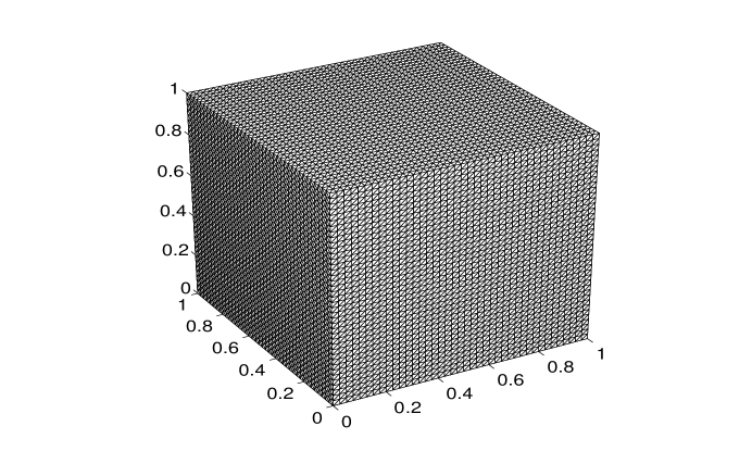
Figure 1: The three-dimensional mesh (Example 4.2).

Table 6: $L^{2}$ Errors of linear FEM with $h=\tau=1/M$ (Example 4.2).

		$\|U_{h}^{n}-u(\cdot,t_{n})\|_{L^{2}}$
$t$	$M=10$	$M=20$	$M=40$	order
1.0	1.1089e-03	2.8319e-04	7.1320e-05	1.9793
2.0	8.6316e-04	2.2523e-04	5.6987e-05	1.9605
3.0	4.0520e-04	1.0626e-04	2.6895e-05	1.9566
4.0	3.6125e-04	9.4243e-05	2.3822e-05	1.9613
		$\|\Phi_{h}^{n}-\phi(\cdot,t_{n})\|_{L^{2}}$
$t$	$M=10$	$M=20$	$M=40$	order
1.0	4.0129e-04	1.1562e-04	2.9779e-05	1.8761
2.0	7.8577e-04	2.1723e-04	5.5611e-05	1.9103
3.0	7.7231e-04	2.1482e-04	5.5087e-05	1.9047
4.0	5.0533e-04	1.4801e-04	3.8404e-05	1.8589

Table 7: $L^{2}$ Errors of linear FEM with $h=1/M$ and $\tau=kh$ (Example 4.2)

		$\|U_{h}^{n}-u(\cdot,t_{n})\|_{L^{2}}$
$t$	$k=1$	$k=5$	$k=10$
1.0	7.1320e-05	2.5286e-04	2.3962e-03
2.0	5.6987e-05	2.4133e-04	1.6463e-03
3.0	2.6895e-05	1.0359e-04	8.5356e-04
4.0	2.3822e-05	2.6147e-04	1.1001e-03
		$\|\Phi_{h}^{n}-\phi(\cdot,t_{n})\|_{L^{2}}$
$t$	$k=1$	$k=5$	$k=10$
1.0	2.9779e-05	2.7311e-04	4.6730e-04
2.0	5.5611e-05	1.2094e-04	1.3614e-03
3.0	5.5087e-05	1.0514e-04	1.7040e-03
4.0	3.8404e-05	1.0333e-04	1.6532e-03

6 Conclusions

We have presented an uncoupled and linearized Crank–Nicolson Galerkin finite element method for the nonlinear time-dependent thermistor equations in the $d$-dimensional space ($d=2,3$) and provided unconditionally optimal error estimates in both $L^{2}$ and $H^{1}$ norms, while existing analysis requires certain time-step restrictions. Our numerical results confirm our analysis and show that the proposed scheme is efficient. Our approach presented in this paper can be extended to many other nonlinear parabolic systems, high-order finite element approximations and other time discretization schemes, while the analysis only focuses on the electric heating model with a linear finite element method to illustrate our idea.

References

[1]
S. Agmon, A. Douglis, and L. Nirenberg, Estimates near the boundary for solutions of
elliptic partial differential equations satisfying general boundary conditions,
Part I and Part II, Comm. Pure Appl. Math., 12 (1959), 623–727; 127 (1964), 35–92.
[2]
G. Akrivis and S. Larsson, Linearly implicit finite element methods
for the time dependent Joule heating problem, BIT, 45 (2005),
429–442.
[3]
W. Allegretto and H. Xie, Existence of solutions for the time
dependent thermistor equation, IMA. J. Appl. Math., 48 (1992),
271–281.
[4]
W. Allegretto and N. Yan, A posteriori error analysis for FEM of
thermistor problems, Int. J. Numer. Anal. Model., 3 (2006),
413 – 436.
[5]
W. Allegretto, Y. Lin and S. Ma, Existence and long time behaviour
of solutions to obstacle thermistor equations,
Discrete and Continuous Dynamical Syst., Series A, 8 (2002), 757–780.
[6]
W. Bao and Y. Cai, Uniform error estimates of finite difference methods
for the nonlinear Schrödinger equation with wave operator,
SIAM J. Numer. Anal., 50 (2012), 492–521.
[7]
S.S. Byun and L. Wang, Elliptic equations with measurable
coefficients in Reifenberg domains, Advances in Mathematics,
225 (2010), 2648–2673.
[8]
J.R. Cannon and Y. Lin, Nonclassical projection and Galerkin
methods for nonlinear parabolic integro-differential equations, Calcolo, 25 (1988), 187–201.
[9] Z. Chen and K. -H. Hoffmann, Numerical studies of a non-stationary
Ginzburg-Landau model for superconductivity, Adv. Math. Sci. Appl.,
5(1995), 363-389.
[10]
G. Cimatti, Existence of weak solutions for the nonstationary
problem of the Joule heating of a conductor, Ann. Mat. Pura
Appl., 162 (1992), 33–42.
[11]
Ya-Zhe Chen and Lan-Cheng Wu, Second Order Elliptic Equations and
Elliptic Systems, Translations of Mathematical Monographs 174, AMS
1998, USA.
[12]
Z. Deng and H. Ma, Optimal error estimates of the Fourier spectral
method for a class of nonlocal, nonlinear dispersive wave equations,
Appl. Numer. Math., 59 (2009), 988–1010.
[13]
T. Dupont, G. Fairweather and J.P. Johnson,
Three-level Galerkin methods for parabolic equations,
SIAM J. Numer. Anal., 11(1974), 392–410.
[14]
C.M. Elliott, and S. Larsson, A finite element model for the
time-dependent Joule heating problem, Math. Comp., 64 (1995),
1433–1453.
[15]
R.E. Ewing and M.F. Wheeler, Galerkin methods for miscible
displacement problems in porous media, SIAM J. Numer. Anal.,
17 (1980), 351–365.
[16]
Yinnian He, The Euler implicit/explicit scheme for the 2D
time-dependent Navier-Stokes equations with smooth or non-smooth
initial data, Math. Comp., 77 (2008), 2097–2124.
[17]
Y. Hou, B. Li and W. Sun,
Error analysis of splitting Galerkin methods
for heat and sweat transport in textile materials,
SIAM J. Numer. Anal., 2012, accepted.
[18]
B. Kellogg and B. Liu, The analysis of a finite element method for
the Navier–Stokes equations with compressibility, Numer.
Math., 87 (2000), 153–170.
[19]
O.A. Ladyzenskaja, V.A. Solonnikov, and N.N. Uralceva, Linear
and quasilinear equations of parabolic type, Translations of
Mathematical Monographs 23, Providence, 1968.
[20]
B. Li and W. Sun,
A new approch to errror analysis of linearized semi-implicit Galerkin
FEMs for nonlinear parabolic equations,
Int. J. Numer. Anal. Model., 2012, accepted.
[21]
B. Li and W. Sun,
Unconditional convergence and optimal error estimates of a
Galerkin-mixed FEM for incompressible miscible flow in porous media,
submitted.
[22]
B. Li,
Mathematical modeling, analysis and computation for some complex and
nonlinear flow problems,
PhD Thesis, City University of Hong Kong, Hong Kong, June, 2012.
[23]
B. Liu, The analysis of a finite element method with streamline
diffusion for the compressible Navier–Stokes equations, SIAM
J. Numer. Anal., 38 (2000), 1-16.
[24]
H. Ma and W. Sun, Optimal error estimates of the
Legendre-Petrov-Galerkin method for the Korteweg-de Vries equation,
SIAM J. Numer. Anal., 39 (2001), 1380–1394.
[25] M. Mu and Y. Huang, An alternating Crank-Nicolson method for
decoupling the Ginzburg-Landau equations, SIAM J. Numer. Anal.,
35(1998), 1740-1761.
[26]
R. Rannacher and R. Scott, Some optimal error estimates for
piecewise linear finite element approximations, Math. Comp.,
38 (1982), 437–445.
[27]
C.G. Simader, On Dirichlet Boundary Value Problem. An Theory
Based on a Generalization of Garding’s Inequality, Lecture Notes in
Math., vol. 268, Springer, Berlin, 1972.
[28]
W. Sun and Z. Sun, Finite difference methods for a nonlinear and
strongly coupled heat and moisture transport system in textile
materials, Numer Math., 120 (2012), 153-187.
[29]
V. Thomée, Galerkin finite element methods for parabolic
problems, Springer-Verkag Berkub Geudekberg 1997.
[30]
Y. Tourigny,
Optimal estimates for two time-discrete Galerkin approximations of
a nonlinear Schrödinger equation,
IMA J. Numer. Anal., 11(1991), 509-523.
[31]
H. Wang, An optimal-order error estimate for a family of ELLAM-MFEM
approximations to porous medium flow, SIAM J. Numer. Anal., 46
(2008), 2133–2152.
[32]
K. Wang, Y. He and Y. Shang, Fully discrete finite element method
for the viscoelastic fluid motion equations, Discrete Contin.
Dyn. Syst. Ser. B, 13 (2010), 665–684.
[33]
M.F. Wheeler, A priori error estimates for Galerkin
approximations to parabolic partial differential equations, SIAM J. Numer. Anal., 10 (1973), 723–759.
[34]
H. Wu, H. Ma and H. Li, Optimal error estimates of the
Chebyshev-Legendre spectral method for solving the generalized
Burgers equation, SIAM J. Numer. Anal., 41 (2003), 659–672.
[35]
X.Y. Yue, Numerical analysis of nonstationary thermistor problem,
J. Comput. Math., 12 (1994), 213–223.
[36]
G. Yuan, Regularity of solutions of the thermistor problem, Appl. Anal., 53 (1994), 149–155.
[37]
G. Yuan and Z. Liu, Existence and uniqueness of the
solution for the thermistor problem with mixed boundary value, SIAM J. Math. Anal., 25 (1994), 1157–1166.
[38]
W. Zhao, Convergence analysis of finite element method for the
nonstationary thermistor problem, Shandong Daxue Xuebao, 29
(1994), 361–367.
[39]
S. Zhou and D.R. Westbrook, Numerical solutions of the thermistor
equations, J. Comput. Appl. Math., 79(1997), 101–118.