Universal Dynamical Steps in the Exact Time-Dependent Exchange-Correlation Potential

Abstract

We show that the exact exchange-correlation potential of time-dependent density-functional theory displays dynamical step structures that have a spatially non-local and time non-local dependence on the density. Using one-dimensional two-electron model systems, we illustrate these steps for a range of non-equilibrium dynamical situations relevant for modeling of photo-chemical/physical processes: field-free evolution of a non-stationary state, resonant local excitation, resonant complete charge-transfer, and evolution under an arbitrary field. Lack of these steps in usual approximations yield inaccurate dynamics, for example predicting faster dynamics and incomplete charge transfer.

The vast majority of applications of time-dependent density functional theory (TDDFT) today deal with the calculation of the linear electronic spectra and response of molecules and solids, and provide an unprecedented balance between accuracy and efficiency RG84 ; TDDFTbook12 . The theorems of TDDFT also apply to any real-time electron dynamics, not necessarily starting in a ground-state, and possibly subject to strong or weak time-dependent fields. Time-resolved dynamics are particularly important and topical for TDDFT for two reasons. First, there is really no alternative practical method for accurately describing correlated electron dynamics, and second, many fascinating new phenomena and technological applications lie in this realm. These include: attosecond control of electron dynamics KV08 , photo-induced coupled electron-ion dynamics (for example in describing light-harvesting and artificial photosyntheses), and photo-chemical/physical processes TTRF08 ; GROT09 in general. TDDFT in theory yields all observables exactly, solely in terms of the time-dependent density, however in practice, approximations must be made both for the observable as a functional of the density, and for the exchange-correlation (xc) functional. Thus the question arises as to whether the approximate functionals that have been successful for excitations predict equally well the dynamics in the more general time-dependent context. In particular, the exact xc contribution to the Kohn-Sham (KS) potential at time $t$ functionally depends on the history of the density $n({\bf r},t^{\prime}<t)$, the initial interacting many-body state $\Psi_{0}$, and the choice of the initial KS state $\Phi_{0}$: $v_{\scriptscriptstyle\rm XC}[n;\Psi_{0},\Phi_{0}]({\bf r},t)$. However, almost all calculations today use an adiabatic approximation, $v_{\scriptscriptstyle\rm XC}^{A}=v_{\scriptscriptstyle\rm XC}^{\rm g.s.}[n(t)]$, that inputs the instantaneous density into a ground-state xc functional HK64 ; PK03 , completely neglecting both the history- and initial-state-dependence. Further, the ground-state functional $v_{\scriptscriptstyle\rm XC}^{\rm g.s.}$ must be approximated; hybrid functionals, that mix in a fraction of exact-exchange to an xc functional that otherwise depends locally or semi-locally in space on the density, are most popular for the spectra of molecules, while the spatially local LDA and semi-local GGA’s are most popular for solids (see Ref. TDDFTbook12 and references therein).

Although understanding when such approximations are expected to work well or fail has advanced significantly in the linear response regime TDDFTbook12 , considerably less is known about the performance of approximate TDDFT for general non-linear time-dependent dynamics Baerissue ; HFTA11 ; RN11 . Part of the reason for this is due to the lack of exact, or highly accurate, results to compare with. Moreover, even in the case where an accurate calculation is available, it is very complicated to extract the exact xc potential (although see Refs. RG12 ; NRL12 for significant progress). Thus, it is critical for the reliability of TDDFT for describing fundamental dynamical processes in the applications mentioned earlier, to first test available xc approximations on systems for which the exact xc potential can be extracted. One such case is that of two-electrons in a spin-singlet, chosen to start in a KS single-Slater determinant. We show that, in this case, the usual adiabatic and semi-local approximations typically fail to capture a critical and fundamental structure in the exact correlation potential: a time-dependent step, that has a spatially ultranonlocal and non-adiabatic dependence on the density. This feature is missing in all available TDDFT approximations today. Even the exact adiabatic functional misses this dynamical step structure. This leads to erroneous dynamics, e.g. faster time scales are observed in the adiabatic approximations for examples where the step opposes the density evolution.

For two-electrons in a spin-singlet we choose, as is usually done, the initial KS state as a doubly-occupied spatial orbital, $\phi({\bf r},t)$. Then the exact KS potential for a given density evolution can be found easily HMB02 . In one-dimension (1D), we have

$$v_{\scriptscriptstyle\rm S}(x,t)=-\frac{(\partial_{x}n(x,t))^{2}}{8n^{2}(x,t)}+\frac{\partial^{2}_{x}n(x,t)}{4n(x,t)}-\frac{u^{2}(x,t)}{2}-\int^{x}\frac{\partial u(x^{\prime},t)}{\partial t}dx^{\prime}$$ (1)

where $u(x,t)=j(x,t)/n(x,t)$ is the local “velocity”, $n(x,t)$ is the one-body density, and $j(x,t)$ is the current-density. We numerically solve the exact time-dependent Schrödinger equation for the two-electron interacting wavefunction, obtain $n(x,t)$ and $j(x,t)$, and insert them into Eq. 1. The exchange-potential in this case is simply minus half the Hartree potential, $v_{\scriptscriptstyle\rm X}(x,t)=-v_{\scriptscriptstyle\rm H}(x,t)/2$, with $v_{\scriptscriptstyle\rm H}(x,t)=\int w(x^{\prime},x)n(x^{\prime},t)dx^{\prime}$, in terms of the two-particle interaction $w(x^{\prime},x)$. Therefore, we can directly extract the correlation potential using

$$v_{\scriptscriptstyle\rm C}(x,t)=v_{\scriptscriptstyle\rm S}(x,t)-v_{\rm ext}(x,t)-v_{\scriptscriptstyle\rm H}(x,t)/2\;,$$ (2)

where $v_{\rm ext}(x,t)$ is the external potential applied to the system. The two electrons in all our 1D examples interact via the soft-Coulomb interaction JES88 , $w(x^{\prime},x)=1/\sqrt{(x^{\prime}-x)^{2}+1}$. We use atomic units throughout.

We start the analysis with some purely (or largely) two-state systems, in which the exact interacting time-dependent wavefunction, $|\Psi(t)\rangle$, can be expanded in a basis consisting of the ground-state, $|\Psi_{g}(t)\rangle$, and the first excited singlet state, $|\Psi_{e}(t)\rangle$:

$$|\Psi(t)\rangle=a_{g}(t)|\Psi_{g}\rangle+a_{e}(t)|\Psi_{e}\rangle$$ (3)

where $a_{g}(t)$ and $a_{e}(t)$ are coefficients given by:

$$i\partial_{t}\left({\begin{array}[]{c}a_{g}(t)\\ a_{e}(t)\\ \end{array}}\right)=\left({\begin{array}[]{cc}E_{g}-d_{gg}{\cal E}(t)&-d_{eg}{\cal E}(t)\\ -d_{eg}{\cal E}(t)&E_{e}-d_{ee}{\cal E}(t)\\ \end{array}}\right)\left({\begin{array}[]{c}a_{g}(t)\\ a_{e}(t)\end{array}}\right)$$ (4)

where $E_{g}$, $E_{e}$ are the energy eigenvalues of the two states, $d_{ab}=\int\Psi_{a}^{*}(x_{1},x_{2})(x_{1}+x_{2})\Psi_{b}(x_{1},x_{2})dx_{1}dx_{2}$ is the transition dipole moment and ${\cal E}(t)=A\cos(\omega t)$ is an applied electric field of strength $A$ and frequency $\omega$. In the weak amplitude limit, with $\omega\gg|d_{eg}A|$ and $\omega$ close to the resonant frequency, this reduces to the textbook Rabi problem. When on-resonance, the system oscillates from one state to the other over a Rabi cycle of period $T_{R}=2\pi/(|d_{eg}|A)$. By solving Eq. 4 we can easily construct the current and density at any time, their time-derivatives, and hence all pieces entering Eq. 1.

In our first example, we consider a “1D He atom”, where $v_{\rm ext}=-2/\sqrt{x^{2}+1}$, subject to a weak electric field of strength $A=0.00667$au and frequency $\omega=0.533$au, resonant with the first singlet excitation RB09 ; FHTR11 . Figure 1 shows snapshots of the correlation potential over one Rabi cycle, while Fig. 2 shows snapshots over one optical period centered around $T_{R}/4$. (Note that the system is not exactly periodic over the Rabi period as the two time-scales dictated by the optical frequency and the Rabi frequency are not commensurate).

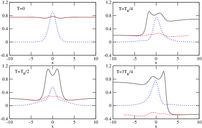
Figure 1: (color online). Snapshots of the exact correlation potential (solid black), density (blue dotted), and exact-adiabatic (red dashed) over one Rabi cycle; at $T_{R}/2$ the density of the first excited state is essentially exactly reached. In all graphs in this paper, the correlation potentials are plotted up to an arbitrary irrelevant time-dependent constant.

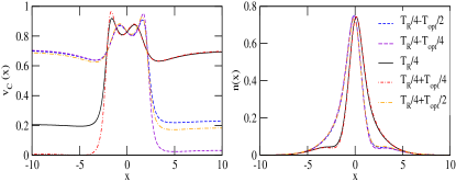
Figure 2: (color online) Snapshots of the correlation potential (left), and corresponding density (right), at times indicated in the right panel.

The most salient feature of the correlation potential is the presence of time-dependent steps, that oscillate on the time-scale of the optical field. These steps arise from the fourth term of Eq. 1: whenever there is a net “acceleration”, $\partial_{t}u(x,t)$, through the system, the spatial-integral is finite, resulting in a potential rising from one end of the system to the other. The correlation potential thus has a spatially ultranonlocal dependence on the density, as it changes far from the system.

Further, the time-dependence of the steps is non-adiabatic, meaning that the instantaneous density is not enough to determine the correlation potential functional. This is clear from Figure 2 where the small changes of the density between time steps cannot capture the observed large changes of the step. One is tempted to point to the time-derivatives in the fourth term in Eq. 1 as further evidence for the non-adiabatic dependence, however caution would be needed for such an argument as time non-locality in $v_{\scriptscriptstyle\rm S}$ is not the same as time non-locality in $v_{\scriptscriptstyle\rm C}$ TDDFTbook12 : the fourth term, for example, may be written as $v_{\rm ext}$ plus other terms, and although $v_{\rm ext}$ has typically strongly non-adiabatic dependence, this is irrelevant because it is never approximated as a functional in practice MLB08 ; TDDFTbook12 , rather it is taken from the problem at hand. Only the xc potential must be approximated, and the functional-dependence of this cannot be deduced directly from Eq. (1). Instead, to unambiguously show the non-adiabatic dependence of the step, we plot the “adiabatically-exact” correlation potential in Fig. 1. This is defined by the exact correlation potential for which both the interacting and KS wavefunctions are ground-state wavefunctions with density equal to the instantaneous one i.e. $v_{\scriptscriptstyle\rm C}^{adia-ex}[n]=v_{\scriptscriptstyle\rm S}^{adia}[n]-v_{\rm ext}^{adia}[n]-v_{\scriptscriptstyle\rm H}[n]-v_{\scriptscriptstyle\rm X}[n]$ TGK08 , where $v_{\rm ext}^{adia}[n]$ is the external potential for two interacting electrons whose ground-state has density $n$, and $v_{\scriptscriptstyle\rm S}^{adia}[n]$ is the exact ground-state KS potential for this density (given by the first two terms in Eq.(1). We find $v_{\rm ext}^{adia}[n]$ using similar techniques to Ref. TGK08, (see also Ref. EM12, ). Fig. 1 shows that $v_{\scriptscriptstyle\rm C}^{adia-ex}[n]$ indeed does not capture the dynamical step structure.

Before turning to our next example, we verify that the two-state approximation for the dynamics is accurate enough for our purposes. Actually one aspect of the potentials we find is indeed an artifact of the two-state approximation: the correlation potential asymptotically has a slope so to exactly cancel the externally applied electric field. This is because the two-state approximation cannot correctly describe polarization arising from occupying many excited states in time. The KS potential obtained from inverting the two-state approximation must therefore be flat asymptotically, as it cannot describe states that are polarized asymptotically. The field is so weak in our case that this effect is hardly noticeable on the scale of Figs. 1 and 2, but to check that our conclusions regarding the dynamics step structure are unaffected by the two-level approximation, we computed the KS potential using the density, current, and their time-derivatives from the numerically exact wavefunction, found using octopus octopus ; octopus2 . Apart from some extra structure in the tail region (small peaks and steps as we move away from the atom), and the linear field-counteracting term, the correlation potential agrees with that from the two-state model.

Dynamical step features have arisen in TDDFT in earlier studies; Refs. LK05 ; TGK08 showed they appear in ionization processes, and linked them to a time-dependent derivative discontinuity, related to fractional charges. In time-resolved transport, step structures have been shown to be essential for describing Coulomb-blockade phenomena KSKV10 , again related to the discontinuity. In the response regime, field-counteracting steps develop across long-range molecules GSGB99 . In open-systems-TDDFT, Ref. TA11 shows steps arise when using a closed KS system to model an open interacting one. In the linear response regime, the xc kernel for charge-transfer excitations displays frequency-dependent steps HG12 . However we argue that the dynamical step structures we are seeing are generic, and moreover, unlike most of the above cases LK05 ; TGK08 ; KSKV10 ; GSGB99 , cannot be captured by an adiabatic approximation. They appear with no need for ionization nor subsystems of fractional charge, nor any applied field (see next example), unlike in Refs. LK05 ; TGK08 ; KSKV10 ; GSGB99 . In this sense our results are more akin to Ref. RG12 , which studies the physically very different situation when an electron freely propagates through a wire. The range of the examples we present suggests that such non-adiabatic and non-local steps generically arise when dealing with real electron dynamics.

Our second example accentuates the fact that dynamical step structures need neither ionization nor an external field to appear. We begin in an equal linear superposition of the ground and first-excited state of the 1D He and let it evolve freely, so that

$$|\Psi(t)\rangle=\left(e^{-iE_{g}t}|\Psi_{g}\rangle+e^{-iE_{e}t}|\Psi_{e}\rangle\right)/\sqrt{2}\;.$$ (5)

It will oscillate back and forth between the two states with frequency $\omega_{0}=E_{e}-E_{g}$. The two-state approximation for this is exact at all times. Again, we see large steps in the correlation potential, as shown in Fig. 3. To support the discussion and provide a microscopic insight behind this phenomenon, we also plot in Fig. 3 the acceleration, $a(x,t)=\partial_{t}u(x,t)$, and its spatial integral with the external potential subtracted out. The position and magnitude of the step at each time is heavily dependent on this term. Peaks in the acceleration, when integrated, become local steps in the potential and the asymptotic value of the step in $v_{\scriptscriptstyle\rm C}(x,t)$ is given by the total step in the spatial integral of $a(x,t)$. Although local step-like features may be cancelled out by the other terms in Eq. (1), the net magnitude of the step is determined from the asymptotic values of this integral.

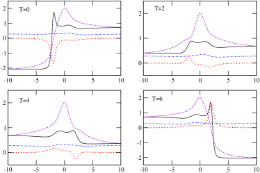
Figure 3: (color online) The exact correlation potential (black solid) shown at times 0, 2, 4, and 6 au, for the two-state example (Eq. 5). Also shown are the local acceleration (red dotted), $\int^{x}\partial_{t}u-v_{\rm ext}$ (purple dashed), and the adiabatically-exact correlation potential (blue dash-dot).

Note that we have the freedom to choose the initial state of the KS system as long as it has the same density and first derivative in time of the exact density L99 , and the shape of the exact correlation potential depends on this choice EM12 . We used a doubly occupied orbital in the previous example, so that we can calculate the exact $v_{\scriptscriptstyle\rm C}$ using the method discussed. A different choice, with a configuration more similar to that of the interacting initial state could well yield a more gentle correlation potential EM12 , with less dramatic step structure.

The generality of the step feature in dynamics is further supported by considering different resonant excitations. Consider a double-well as a model of a molecule:

$$v_{\rm ext}(x,t)=-\frac{2}{\sqrt{(x+3.5)^{2}+1.0}}-\frac{1}{\cosh^{2}(x-3.5)}-{\cal E}(t)x$$ (6)

with ${\cal E}(t)=0.006\cos(0.112t)$. Here the ground-state has two electrons in one well, and a charge-transfer excited state $\Psi_{e}$, with one electron in each well, at a frequency of 0.112au. We use the ground-state and $\Psi_{e}$ in the two-state model of Eq. (3), and solve for the occupations using Eq. (4); we again checked the two-state result against the exact numerical solution using octopus. The system behaves like the Rabi problem with non-zero dipole moment for the ground-state KM85 ; BMT00 . In Fig. 4 we plot the correlation potential for several times within an optical cycle around $T_{R}/8$. Again dynamical steps oscillating on the optical frequency time scale emerge. The situation is more complicated as a step related to the delocalization of the density during the charge-transfer process slowly develops (on the time-scale of $T_{R}/2$) FERM12 . The dynamical step can then increase, decrease, or even reverse this charge-transfer step. Approximations unable to develop steps lead to incomplete charge-transfer. This, along with other details of time resolved charge-transfer, is investigated in more detail in Ref. FERM12 . For our purposes, it is sufficient to note that dynamical steps are again present to capture the exact dynamics.

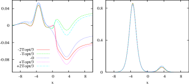
Figure 4: (color online) The correlation potential (left) and density (right) shown at snapshots of time $T_{R}/8\pm$ fractions of the optical period, $T_{\rm opt}=2\pi/0.112$au, that are indicated in the key, for the two-well potential model Eq. (6).

Finally, we explicitly demonstrate that the non-local non-adiabatic step feature is a generic aspect of the correlation potential in the following way. We subject the 1D He atom to an electric field that is chosen somewhat arbitrarily: it is relatively strong and linearly switched on over 2 optical cycles, with an off-resonant frequency. In Fig. 5, we show the exact correlation potential at four times, along with the density, and the adiabatically-exact correlation potential. The time-dependent step in the exact $v_{\scriptscriptstyle\rm C}$ is once again evident, and again fails to be captured by the adiabatically-exact approximation.

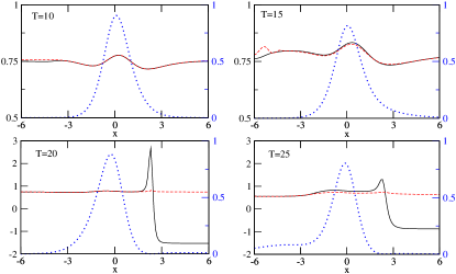
Figure 5: (color online). The exact correlation potentials (solid, black) at times $10$,$15$,$20$,$25$au during propagation under $\mathcal{E}(t)=\frac{t}{2\sqrt{2}}\frac{0.3}{4\pi}\cos(0.3\ t)$. Also shown are the adiabatically-exact correlation potentials (dashed red), and the density (dotted blue, scale on the right).

In summary, dynamical steps in the correlation potential are a generic feature of electron dynamics. The step features discussed above arise from part of the fourth term of Eq. (1), which suggests that any time there is a net localized acceleration, there will be a step, and that it will have a very non-local spatial dependence on the density, and is non-adiabatic. This represents a type of time-dependent screening, where the electron-electron interaction hinders electron movement to certain regions. Although two-electron systems were studied here, we expect steps are a more general feature of electron dynamics, as supported by the recent Ref. RG12 .

The lack of the step in approximations leads to incorrect dynamics. For example, faster time scales in adiabatic approximations were found for the field-free dynamics of a linear superposition state, where the direction of the step tended to oppose the density’s motion. The exact dipole and adiabatic exact-exchange (AEXX) dipole for this case are shown in Fig. 6. We computed the dynamics of the the local excitation in Figs 1 and 2 using AEXX, adiabatic LDA, and adiabatic self-interaction-corrected LDA. In all cases, we found the timescale for the dipole oscillations was faster than in the true case, in spite of providing good linear response spectra FHTR11 . How general this finding is will be investigated in future work.

We note that the xc electric field, defined as the gradient of the xc potential, has a more local character than the potential. This suggests that considering functional approximations to this field, or, more generally, to an xc vector potential VK96 ; RG12 , may point to an easier path to develop approximations containing step features.

As applications of TDDFT continue to expand, it is crucial to further study what the impact of the missing steps in the approximations are on the predictions of these calculations. When starting in the ground-state, the exact adiabatic potential may follow well the exact dynamics at short times, but as soon as there is an appreciable change in the occupation of an excited state, the exact soution develops the dynamical step, entirely missing in the adiabatic one. This result is general and applies to all available functionals. It raises an important issue when applying TDDFT to fundamental photo-induced processes (e.g. photovoltaics, artificial photosynthesis, photoactivated chemistry, photophysics, etc): all these involve a significant change of state population. Clearly population of many-body states due to the external field is not a linear process and requires functionals able to cope with the generic features of the dynamical step that we have unveiled in the present work.

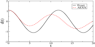
Figure 6: (color online). The dipole moments in the field-free propagation of the linear-superposition state (see text), where the TDKS calculation starts in the exact singlet doubly occupied orbital initial state.

Acknowledgments Financial support from the National Science Foundation (CHE-1152784), and a grant of computer time from the CUNY High Performance Computing Center under NSF Grants CNS-0855217 and CNS-0958379, are gratefully acknowledged. JIF acknowledges support from an FPI-fellowship (FIS2007-65702-C02-01). AR acknowledge financial support from the European Research Council Advanced Grant DYNamo (ERC-2010-AdG -Proposal No. 267374) Spanish Grants (FIS2011-65702- C02-01 and PIB2010US-00652), Grupos Consolidados UPV/EHU del Gobierno Vasco (IT-319-07), and European Commission project CRONOS (280879-2)

References

- (1) E. Runge and E.K.U. Gross, Phys. Rev. Lett. 52, 997 (1984).
- (2) Fundamentals of Time-Dependent Density Functional Theory, (Lecture Notes in Physics 837), eds. M.A.L. Marques, N.T. Maitra, F. Nogueira, E.K.U. Gross, and A. Rubio, (Springer-Verlag, Berlin, Heidelberg, 2012); and references therein.
- (3) M. F. Kling and M. J. J. Vrakking, Annu. Rev. Phys. Chem. 59, 463 (2008).
- (4) E. Tapavicza, I. Tavernelli, U. Rothlisberger, C. Filippi, and M. E. Casida, J. Chem. Phys. 129, 124108 (2008).
- (5) J. Gavnholt, A. Rubio, T. Olsen, K. S. Thygesen, and J. Schiøtz, Phys. Rev. B 79, 195405 (2009).
- (6) P. Hohenberg and W. Kohn, Phys. Rev. 136, B864 (1964).
- (7) J. P. Perdew and S. Kurth, in Lecture Notes in Physics 620, eds. C. Fiolhas, F. Nogueira, M. Marques (Springer-Verlag, Berlin Heidelberg, 2003).
- (8) Special Issue on ”Open Problems and new solutions in time dependent density functional Theory”, Chemical Physics 391, eds. R. Baer, L. Kronik, S. Kuemmel. (2011).
- (9) N. Helbig, J.I. Fuks, I.V. Tokatly, H. Appel, E.K.U. Gross, A. Rubio Chemical Physics 391, 1 (2011).
- (10) S. Raghunathan and M. Nest, J. Chem. Theory and Comput. 7, 2492 (2011).
- (11) J. D. Ramsden and R. W. Godby, Phys. Rev. Lett. 109, 036402 (2012).
- (12) S. E. B. Nielsen, M. Ruggenthaler, R. van Leeuwen, arXiv:1208.0226v2
- (13) P. Hessler, N. T. Maitra, and K. Burke, J. Chem. Phys. 117, 72 (2002).
- (14) J. Javanainen, J. H. Eberly, Q. Su, Phys. Rev. A. 38, 3430 (1988).
- (15) M. Ruggenthaler and D. Bauer, Phys. Rev. Lett. 102, 233001 (2009).
- (16) J. I. Fuks, N. Helbig, I. V. Tokatly, and A. Rubio, Phys. Rev. B. 84, 075107 (2011).
- (17) N. T. Maitra, R. van Leeuwen, and K. Burke, Phys. Rev. A 78, 056501 (2008).
- (18) M. Thiele, E. K. U. Gross, and S. Kümmel, Phys. Rev. Lett. 100, 153004 (2008).
- (19) P. Elliott and N. T. Maitra, Phys. Rev. A. 85, 052510 (2012).
- (20) A. Castro et al., Phys. Stat. Sol. (b) 243, 2465 (2006).
- (21) M. A. L. Marques, A. Castro, G. F. Bertsch, and A. Rubio, Comp. Phys. Comm. 151, 60 (2003).
- (22) M. Lein and S. Kümmel, Phys. Rev. Lett. 94, 143003 (2005).
- (23) S. Kurth, G. Stefanucci, E. Khosravi, C. Verdozzi, and E. K. U. Gross, Phys. Rev. Lett. 104, 236801 (2010).
- (24) S.J.A. van Gisbergen, P.R.T. Schipper, O.V. Gritsenko, E.J. Baerends, J.G. Snijders, B. Champagne, B. Kirtman, Phys. Rev. Lett. 83, 694 (1999).
- (25) D. G. Tempel and A. Aspuru-Guzik, Chem. Phys. 391, 130 (2011).
- (26) M. Hellgren and E. K. U. Gross, Phys. Rev. A. 85, 022514 (2012).
- (27) R. van Leeuwen, Phys. Rev. Lett. 82, 3863 (1999).
- (28) M. A. Kmetic and W. J. Meath, Phys. Lett. A 108, 340 (1985).
- (29) A. Brown, W.J. Meath, P. Tran, Phys REVIEW A, VOLUME ,(2000)
- (30) J. I. Fuks, P. Elliott, A. Rubio, and N. T. Maitra, in prep.
- (31) G. Vignale and W. Kohn, Phys. Rev. Lett. 77, 2037 (1996).