Forward jet production & quantum corrections to the gluon Regge trajectory from Lipatov’s high energy effective action

Abstract

We review Lipatov’s high energy effective action and show that it is a useful computational tool to calculate scattering amplitudes in (quasi)-multi-Regge kinematics. We explain in some detail our recent work where a novel regularization and subtraction procedure has been proposed that allows to extend the use of this effective action beyond tree level. Two examples are calculated at next-to-leading order: forward jet vertices and the gluon Regge trajectory.

1 Introduction

A useful description of the high energy limit of perturbative QCD can be given in terms of high energy factorization and the BFKL evolution equation. In this framework large logarithms in the center of mass energy $\sqrt{s}$ at leading (LL) [1] and next-to-leading logarithmic (NLL) accuracy [2] are resummed. Applications of this framework to LHC and HERA phenomenology are numerous, for recent results see [3]. The building block in this formalism is the realization that QCD scattering amplitudes in the high energy limit are dominated by the exchange of an effective $t$-channel degree of freedom, the so-called reggeized gluon, which couples to the external scattering particles through process dependent effective vertices. The calculation of higher order corrections to both the effective couplings and the reggeized gluon propagators is a difficult task. This is especially true when attempting to go beyond LL accuracy, with the aim to obtain accurate phenomenological predictions.

A powerful tool to easy these calculations is provided by Lipatov’s high energy effective action [4], which corresponds to the usual QCD action with the addition of an induced term containing the new effective degrees of freedom relevant in this limit. This induced piece is written in terms of gauge-invariant currents which generate a non-trivial coupling of the gluon to the reggeized gluon fields. Tree level amplitudes at high energies have been obtained making use of this action in Ref. [5]. Loop corrections are technically more involved since a new type of longitudinal divergences, not present in conventional QCD amplitudes, appear. The treatment of these divergences has been addressed for LL transition kernels in Ref. [6] while the coupling for one to two reggeized gluons with the associated production of an on-shell gluon has been studied in [7]. Recently, this high energy effective action has been used for the first time for the calculation of NLL corrections to the forward quark-initiated jet vertex [9] and the quark contribution to the two-loop gluon trajectory [8], finding exact agreement with previous results in the literature. In the following we review the key steps to perform these calculations.

2 High energy factorization and the effective action

Following Lipatov’s work [4] in this section we motivate the construction of gauge invariant high energy factorization and the effective action from an explicit study of QCD tree-level amplitudes.

To fix our notation let us use the partonic scattering process $p_{A}+p_{B}\to p_{1}+p_{2}+\ldots$, with light-like initial momenta $p_{A}^{2}=p_{B}^{2}=0$ and squared center of mass energy $s=2p_{A}\cdot p_{B}$. Dimensionless light-cone four-vectors $n^{+}$ and $n^{-}$ are then defined through the following rescaling $n^{+}=2p_{B}/\sqrt{s}$ and $n^{-}=2p_{A}/\sqrt{s}$. The general Sudakov decomposition of a four vector $k^{\mu}$ can then be written in the form

$$k^{\mu} =\frac{k^{+}}{2}(n^{-})^{\mu}+\frac{k^{-}}{2}(n^{+})^{\mu}+{\bm{k}}^{\mu}, k^{\pm} =n^{\pm}\cdot k, n^{\pm}\cdot{\bm{k}}=0.$$ (1)

We start with the simpler example of a scalar $\phi^{3}$-theory. The tree-level diagrams for a $2\to 2$ scattering process are

$$=\parbox{56.9055pt}{\includegraphics[width=71.13188pt]{phi3t.pdf}}\quad+\quad\parbox{56.9055pt}{\includegraphics[width=71.13188pt]{phi3s.pdf}}\quad+\quad\parbox{56.9055pt}{\includegraphics[width=71.13188pt]{phi3u.pdf}}\leavevmode\nobreak\ \leavevmode\nobreak\ \leavevmode\nobreak\ \leavevmode\nobreak\ \leavevmode\nobreak\ .$$ (2)

In this case the high energy limit $s\sim-u\gg-t$ with $t=q^{2}$, $q=p_{b}-p_{2}$ and $u=(p_{a}-p_{2})^{2}$ is driven by the first diagram of the sum in Eq. (2), while the $s$- and $u$-channel diagrams are power-suppressed with energy. In these kinematics the ‘plus’ (‘minus’) momenta of the upper (lower) particles in the diagram are conserved, $p_{a}^{+}\simeq p_{1}^{+}$ and $p_{b}^{-}\simeq p_{2}^{-}$, which implies that the $t$-channel momentum $q$ takes for the ‘upper’ particles with momenta $p_{a}$ and $p_{1}$ the effective form

$$q =\frac{q^{-}}{2}n^{+}+{\bm{q}} \text{(region a-1)},$$ (3)

while for the lower particles with momenta $p_{b}$ and $p_{2}$ we have

$$q =\frac{q^{+}}{2}n^{-}+{\bm{q}} \text{(region b-2)}.$$ (4)

In QCD a similar process is given by elastic gluon-quark scattering ($g(p_{a})q(p_{b})\to g(p_{1})g(p_{2})$) with the following diagrams

$$=\parbox{85.35826pt}{\includegraphics[width=85.35826pt]{gq_qcd1.pdf}}+\parbox{85.35826pt}{\includegraphics[width=85.35826pt]{gq_qcd2.pdf}}+\parbox{85.35826pt}{\includegraphics[width=85.35826pt]{gq_qcd3.pdf}}.$$ (5)

Kinematics carries over from the $\phi^{3}$-theory, with the additional feature that for covariant gauges certain longitudinal components of the gauge fields are enhanced in comparison to their transverse counterparts. In particular, in covariant Feynman gauge, the polarization tensor of the $t$-channel gluon is to be replaced by its enhanced longitudinal part $g_{\mu\nu}\to n^{+}_{\mu}n^{-}_{\nu}/2$ while the $s$-channel gluons emitted directly from the quark line have, up to power suppressed corrections, polarizations proportional to $n^{+}_{\mu}$.

In contrast to kinematical effects, for which QCD and the scalar theory agree, the gauge theory nature of QCD no longer allows to drop the contribution from the $s$- and $u$-channel diagrams. While certain choices such as the $V\cdot n^{+}=0$ light-cone gauge allow to cast the entire relevant contributions into the $t$-channel diagram, gauge invariance requires to take into account the full set of diagrams in Eq. (5). Naïve high energy factorization at the level of QCD Feynman diagrams therefore no longer occurs.

Within the effective action proposed in [4] this problem is solved by introducing an additional effective scalar degree-of-freedom which describes the interaction between particles with significantly different rapidity $y=1/2\ln(k^{+}/k^{-})$. Due to its scalar nature, this degree-of-freedom (which is identified with the reggeized gluon) is invariant under gauge transformations and sets the basis for gauge invariant high energy factorization. Building on the $\phi^{3}$-theory result and on the observation that the $V\cdot n^{+}=0$ gauge still allows to describe the entire process in terms of the $t$-channel contributions only, the effective action formalism takes as a starting point the QCD $t$-channel topologies. As a second step these contributions are dressed, making use of new ‘induced vertices’ , with precisely those contributions of the QCD $s$- and $u$-channel diagrams which are needed to restore gauge invariance.

The elastic gluon-quark scattering amplitude in the high energy limit is then described by the following set of diagrams

$$=\parbox{85.35826pt}{\includegraphics[width=85.35826pt]{gq_eff1.pdf}}+\parbox{85.35826pt}{\includegraphics[width=85.35826pt]{gq_eff2.pdf}}+\mathcal{O}\left(\frac{|t|}{s}\right).$$ (6)

The Feynman rules needed for the construction of these diagrams are shown in Fig. 1.

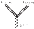
$=\displaystyle\begin{array}[h]{ll}\\ \\ -i{\bm{q}}^{2}\delta^{ac}(n^{\pm})^{\nu},\\ \\ \qquad k^{\pm}=0.\end{array}$ $=\displaystyle\begin{array}[h]{ll}\delta^{ab}\frac{i/2}{{\bm{q}}^{2}}\end{array}$ $\displaystyle=\begin{array}[h]{ll}\\ \\ gf^{c_{1}c_{2}a}\frac{{\bm{q}}^{2}}{k_{1}^{\pm}}(n^{\pm})^{\nu_{1}}(n^{\pm})^{\nu_{2}},\\ \\ \quad k_{1}^{\pm}+k_{2}^{\pm}=0\end{array}$
(a) (b) (c)

Figure 1: Transition vertex (a), reggeized gluon propagator (b) and induced vertex (c).

The first element, Fig. 1.a, yields the projection of the QCD gluon on the high energy kinematics and polarization. Fig. 1.b describes the propagator of the effective $t$-channel exchange; it agrees with the high energy limit of the $t$-channel gluon propagator in covariant gauge, with polarization vectors $n^{+}_{\mu}n^{-}_{\nu}$ being absorbed into the adjacent vertices. Fig. 1.c corresponds to the $\mathcal{O}(g)$ induced vertex, which makes the two gluon-reggeized gluon amplitude to be gauge invariant. With the latter defined as

$$i\mathcal{M}^{\mu\nu,abc}_{2gr^{*}}(p_{a},p_{1},q) =\parbox{56.9055pt}{\centering\includegraphics[height=51.21504pt]{indu1_lab.pdf}\@add@centering}+\parbox{56.9055pt}{\centering\includegraphics[height=51.21504pt]{3gl_lab.pdf}\@add@centering}$$ (7)

one explicitly finds that the corresponding Slavnov-Taylor identities are fulfilled

$${p_{a}}_{\mu}\mathcal{M}^{\mu\nu}_{2gr^{*}}(p_{a},p_{1},q)\epsilon^{(\lambda)}_{\nu}(p_{1}) =0={p_{a}}_{\mu}\mathcal{M}^{\mu\nu}_{2gr^{*}}(p_{a},p_{1},q){p_{1}}_{\nu},$$

$$\epsilon^{(\lambda)}_{\nu}(p_{a})\mathcal{M}^{\mu\nu}_{2gr^{*}}(p_{a},p_{1},q){p_{1}}_{\nu} =0.$$ (8)

This structure can be extended to the case where $n$-gluons are produced in the fragmentation region of the initial gluon and the whole cluster is well-separated in rapidity from the final state quark, see Fig. 2.

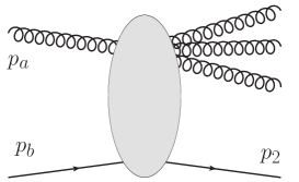
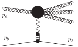
(a)

(b)

Figure 2: a) Quasi-elastic scattering of a gluon on a quark with final state gluons produced in the fragmentation region of the initial gluon, well-separated separated in rapidity from the target quark. b) The effective action formalism factorizes this process with the fragmentation process described by a gauge invariant $n$ gluon-reggeized gluon amplitude.

To achieve gauge invariance for the (tree-level) $n$-gluon–reggeized gluon amplitude, it is needed to supplement the set in Fig. 1 for the $i$th additional external gluon with the corresponding $\mathcal{O}(g^{i+1})$ induced vertex. As a result one obtains a recursive relation for the $\mathcal{O}(g^{n})$ induced vertex; the latter can then be expressed as the $\mathcal{O}(g^{n})$ term of a path order exponential. This fact was first observed in [4, 5] and has been recently rederived in [13].

Lipatov’s effective action generates the above-mentioned set of diagrammatic rules by adding to the QCD action, $S_{\text{QCD}}$, an additional induced term, $S_{\text{ind.}}$, which describes the coupling of the gluonic field $v_{\mu}=-it^{a}v_{\mu}^{a}(x)$ to the reggeized gluon field $A_{\pm}(x)=-it^{a}A_{\pm}^{a}(x)$. We therefore have

$$S_{\text{eff}} =S_{\text{QCD}}+S_{\text{ind.}},$$ (9)

where we include the gauge-fixing and ghost terms

$${S}_{\text{QCD}}=\int d^{4}x\big{[}\mathcal{L}_{\text{QCD}} (v_{\mu},\psi,\bar{\psi})+\mathcal{L}_{\text{fix}}(v_{\mu})+\mathcal{L}_{\text{ghost}}(v_{\mu},\phi,\phi^{\dagger})\big{]}.$$ (10)

The reggeized gluon field obeys the kinematic constraint

$$\partial_{+}A_{-} =0=\partial_{+}A_{+},$$ (11)

in order to fulfill the kinematic conditions in Eqs. (3) and (4). Although the reggeized gluon field is charged under the QCD gauge group SU$(N_{c})$, it is invariant under local gauge transformations, $\delta A_{\pm}=0$. Its kinetic term and the gauge invariant coupling to the QCD gluon field are included in the induced term

$$S_{\text{ind.}}=\int\text{d}^{4}x{\rm tr}\left[\left(W_{-}[v]-A_{-}\right)\partial^{2}_{\perp}A_{+}\right]+{\rm tr}\left[\left(W_{+}[v]-A_{+}\right)\partial^{2}_{\perp}A_{-}\right].$$ (12)

The definition of the non-local functionals $W_{\pm}[v]$ reads

$$W_{\pm}[v]= -\frac{1}{g}\partial_{\pm}U[v_{\pm}]=v_{\pm}-gv_{\pm}\frac{1}{\partial_{\pm}}v_{\pm}+g^{2}v_{\pm}\frac{1}{\partial_{\pm}}v_{\pm}\frac{1}{\partial_{\pm}}v_{\pm}-\ldots$$ (13)

with

$$U[v_{\pm}] =\mathrm{P}\exp\left(-\frac{g}{2}\int^{x^{\pm}}_{-\infty}dz^{\pm}v_{\pm}(z^{\pm},x_{\perp})\right) x_{\perp} =(x^{\mp},{\bm{x}}),$$ and (14)

being a path ordered exponential with an integration contour located along the two light-cone directions and with the boundary condition $\lim_{x^{\pm}\to\infty}U[v_{\pm}]=1$.

While the effective action can be used to generate the necessary set of rules to construct the high energy limit of quasi-elastic amplitudes as discussed in the previous paragraph and depicted in Fig. 2, its range of applicability reaches further. It allows to generate a general production amplitude in quasi-multi-Regge-kinematics (QMRK), see Fig. 3. In this case, besides particle production in the fragmentation region of the initial scattering particles, arbitrary many clusters of particles can be produced at central rapidities, with these clusters being strongly ordered in rapidity among themselves.

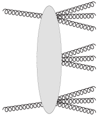
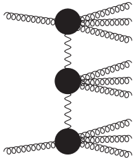
Figure 3: Gluon production in quasi-multi-Regge kinematics. In the effective action framework, each of the clusters separated in rapidity is connected through reggeized gluon exchange.

From Eq. (9) we notice that the high energy effective action does not correspond to an effective field theory in the conventional Wilsonian sense. Since we now have an enhanced set of Feynman diagrams it is needed to device some cut-off or subtraction procedure to avoid double counting in our calculations. In the remaining of this review we explain a convenient method to achieve this in two different calculations.

3 Forward jet vertex at NLO

Let us first use Lipatov’s effective action by applying it to the study of the high energy limit of a simple QCD process at NLO: quark-quark scattering.

3.1 The Born-level result

At Born level the effective action in Eq. (9) provides two Feynman diagrams for the process $p_{a}+p_{b}\to p_{1}+p_{2}$, depicted in Fig. 4.

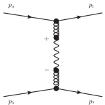
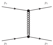
(a)

(b)

Figure 4: Quark-quark scattering mediated by (a): reggeized gluon exchange, (b): gluon exchange.

To determine the Born level cross-section in the high energy limit we need to evaluate diagram Fig. 4.a. It contains the coupling of a reggeized gluon to the on-shell quarks which reads

$$i\mathcal{M}_{qr^{*}\to q}^{(0)} =\parbox{71.13188pt}{\includegraphics[width=85.35826pt]{QQRtrans0.pdf}}=\bar{u}_{\lambda^{\prime}}(p^{\prime})igt^{a}\not{n}^{\pm}u_{\lambda}(p)=igt^{a}2p^{\pm}\delta_{\lambda\lambda^{\prime}}.$$ (15)

Evaluating the differential cross-section

$$d\hat{\sigma}^{(0)}_{q_{a}q_{b}}=h^{(0)}_{a}({{\bm{k}}})h^{(0)}_{b}({\bm{k}})d^{d-2}{\bm{k}}$$ (16)

in $d=4+2\epsilon$ dimensions with the $\overline{\rm MS}$ scheme coupling $\alpha_{s}=\frac{g^{2}\mu^{2\epsilon}\Gamma(1-\epsilon)}{(4\pi)^{1+\epsilon}}$ and $C_{F}=\frac{N_{c}^{2}-1}{2N_{c}}$ we find

$$\overline{|\mathcal{M}^{(0)}|^{2}}_{qr^{*}\to q} =\frac{1}{4N_{c}(N_{c}^{2}-1)}\sum_{\lambda\lambda^{\prime}}|\mathcal{M}^{(0)}|^{2}_{qr^{*}\to q}=\frac{4g^{2}C_{F}}{{N_{c}^{2}-1}}p_{a}^{+2},$$ (17)

and the leading order (LO) quark impact factor $h^{(0)}_{a}({\bm{k}})$ in Eq. (16) is given by

$$h_{a}^{(0)}({\bm{k}})=\frac{C_{F}}{\sqrt{N_{c}^{2}-1}}\frac{2^{1+\epsilon}}{\mu^{2\epsilon}\Gamma(1-\epsilon)}\frac{1}{\bm{k}^{2}},$$ (18)

in agreement with  [14]. The same result can be obtained by evaluating the diagram in Fig. 4.b in the limit $|t|/s\to 0$. In [4] it was suggested to introduce a factorization parameter $\eta$ to associate the high energy region $|t|/s<\eta$ with diagram Fig. 4.a, and the low energy region $|t|/s>\eta$ with Fig. 4.b. Alternatively, it is possible to subtract the high energy cross-section from the QCD diagram in Fig. 4.b. More precisely, if the QCD cross-section reads

$$\left(d\hat{\sigma}_{q_{a}q_{b}}^{(0)}\right)_{\text{QCD}} =\frac{1}{2s}\frac{1}{4N^{2}_{c}}\sum_{\begin{subarray}{c}\text{spin}\\ \text{color}\end{subarray}}\left|\parbox{99.58464pt}{\centering\includegraphics[height=71.13188pt]{4pointLOQCD.pdf}\@add@centering}\right|^{2}d\Phi^{(2)}$$ (19)

where $d\Phi^{(2)}$ denotes the 2 particle Lorentz invariant phase space measure, we can define a low energy coefficient in the form

$$d\hat{\mathcal{C}}_{q_{a}q_{b}}^{(0)} =\left(d\hat{\sigma}_{q_{a}q_{b}}^{(0)}\right)_{\text{QCD}}-d\hat{\sigma}_{q_{a}q_{b}}^{(0)}.$$ (20)

The complete effective action result then consists of the sum of the high energy cross-section in Eq. (16) and the low energy coefficient in Eq. (20) which by construction agrees with the QCD result. The leading term of the high energy expansion of the QCD cross-section is then formally obtained by dropping the low energy contribution in Eq. (20).

This procedure can be applied in general to any class of effective action matrix elements stemming from Eq. (9). From those amplitudes with internal QCD propagators only, to which the reggeized gluon couples as an external (classical) field, one subtracts the corresponding high energy factorized amplitudes with reggeized gluon exchange. The subtracted coefficient is then local in rapidity.

3.2 Real corrections

The real corrections to the Born level process can be organized into three contributions to the five-point amplitude with central and quasi-elastic gluon production:

Integrating over the longitudinal phase space of the produced gluon we will find divergences which can be regularized using an explicit cut-off in rapidity. The central production amplitude, obtained from the sum of the following three effective diagrams, yields the unintegrated real part of the forward LO BFKL kernel:

$$= \parbox{56.9055pt}{\centering\includegraphics[width=34.14322pt]{C1.pdf}\@add@centering}+\parbox{56.9055pt}{\centering\includegraphics[width=34.14322pt]{C2.pdf}\@add@centering}+\parbox{56.9055pt}{\centering\includegraphics[width=34.14322pt]{C3.pdf}\@add@centering},$$

with the following Sudakov decomposition of the momenta

$$k^{\prime}=\frac{q^{+}}{2}n^{+}+{\bm{k}}^{\prime},\qquad k=\frac{k^{-}}{2}n^{+}+\bm{k},\qquad q=\frac{q^{+}}{2}n^{+}+\frac{k^{-}}{2}n^{+}+{\bm{q}},$$ (21)

with

$$k^{-} =\frac{{\bm{q}}^{2}}{q^{+}} {\bm{k}}^{\prime} ={\bm{q}}-{\bm{k}}.$$ (22)

Note that the condition ${k^{\prime}}^{-}=0=k^{+}$ appears as a direct consequence of the kinematic constraint in Eq. (11). The squared amplitude, averaged over color of the incoming reggeized gluons and summed over final state color and helicities reads

$$\overline{|\mathcal{M}|^{2}}_{r^{*}r^{*}\to g} = \frac{16g^{2}N_{c}}{N_{c}^{2}-1}\frac{{\bm{k}^{\prime}}^{2}{\bm{k}}^{2}}{{\bm{q}}^{2}}.$$ (23)

It leads to the following production vertex

$$V({\bm{q}};{\bm{k}},{\bm{k}}^{\prime}) = \frac{N_{c}^{2}-1}{8(2\pi)^{3+2\epsilon}{\bm{k}}^{2}{\bm{k}^{\prime}}^{2}}\overline{|\mathcal{M}|^{2}}_{r^{*}r^{*}\to g}\leavevmode\nobreak\ =\leavevmode\nobreak\ \frac{\alpha_{s}N_{c}}{\mu^{2\epsilon}\pi^{2+\epsilon}{\bm{q}}^{2}}.$$ (24)

The exclusive differential cross section for central production then reads

$$d\hat{\sigma}^{(c)}_{ab} =h^{(0)}_{a}({\bm{k}^{\prime}})h^{(0)}_{b}({\bm{k}})\mathcal{V}({\bm{q}};{\bm{k}},{\bm{k}^{\prime}},\eta_{a},\eta_{b})d^{2+2\epsilon}{\bm{k}^{\prime}}d^{2+2\epsilon}{\bm{k}}\,d\eta,$$ (25)

where ${\cal V}({\bm{q}};{\bm{k}},{\bm{k}^{\prime}},\eta_{a},\eta_{b})\equiv V({\bm{q}};{\bm{k}},{\bm{k}^{\prime}})\theta(\eta_{a}-\eta)\theta(\eta-\eta_{b})$ corresponds to the regularized production vertex with cut-offs $\eta_{a,b}$, to be evaluated in the limit $\eta_{a,b}\to\infty$. Once integrated over the full range in $\eta$, Eq. (25) without regulators would result into a (longitudinal) high energy divergence, proportional to the real part of the LO BFKL kernel.

For the quasi-elastic contribution $q(p_{a})r^{*}(k)\to g(q)q(p)$ we first evaluate the sum of the effective diagrams

$$= \parbox{113.81102pt}{\centering\includegraphics[width=99.58464pt]{QQRt_real1.pdf}\@add@centering}+\parbox{113.81102pt}{\centering\includegraphics[width=99.58464pt]{QQRt_real2.pdf}\@add@centering}$$

$$+ \parbox{113.81102pt}{\centering\includegraphics[width=99.58464pt]{QQRt_real3.pdf}\@add@centering}+\parbox{113.81102pt}{\centering\includegraphics[width=99.58464pt]{QQRt_real4.pdf}\@add@centering}.$$

With the Sudakov decomposition of external momenta given by

$$p_{a} =\frac{p_{a}^{+}}{2}n^{-} p =\frac{(1-z)p_{a}^{+}}{2}n^{-}+\frac{p^{-}}{2}n^{+}+{\bm{k}}-{\bm{q}},$$

$$k =\frac{k^{-}}{2}n^{+}+{\bm{k}} q =\frac{zp_{a}^{+}}{2}n^{-}+\frac{k^{-}-p^{-}}{2}n^{+}+{\bm{q}},$$ (26)

with $z=q^{+}/p^{+}_{a}$ and

$$p^{-} =\frac{({\bm{k}}-{\bm{q}}^{2})}{(1-z)p_{a}^{+}}, k^{-} =\frac{{\bm{\Delta}}^{2}+z(1-z){\bm{k}}^{2}}{(1-z)p_{a}^{+}}, {\bm{\Delta}} ={\bm{q}}-z{\bm{k}}.$$ (27)

The squared amplitude reads

$$\overline{|\mathcal{M}|^{2}}_{r^{*}q\to qg} = \frac{8g^{4}p_{a}^{+2}}{{N_{c}^{2}-1}}\frac{\mathcal{P}_{gq}(z,\epsilon)}{\bm{\Delta}^{2}\bm{q}^{2}}\frac{(1-z)z\bm{k}^{2}}{\bm{k}^{\prime 2}}\theta\left(z-e^{-\eta_{b}}\frac{\sqrt{q_{\perp}^{2}}}{p_{a}^{+}}\right)$$ (28)

$$\qquad\qquad\qquad\qquad\cdot\left[C_{F}z^{2}{k}^{\prime 2}+N_{c}(1-z)\bm{\Delta}\cdot\bm{q}\right],$$

where $\mathcal{P}_{gq}(z,\epsilon)=C_{F}\frac{1+(1-z)^{2}+\epsilon z^{2}}{z}$ is the real part of the $q\to g$ splitting function and ${\bm{k}}^{\prime}={\bm{q}}-{\bm{k}}$. The lower cut-off $\eta_{b}$ on the rapidity $\eta=\ln{\bm{q}}^{2}/(zp_{a}^{+})$ of the gluon has been introduced, in direct analogy to the corresponding lower cut-off for the central production vertex. The upper limit for the quasi-elastic contribution is bounded by kinematics since $z<1$. Putting together these results, the real corrections to the jet vertex are

$$h^{(1)}({\bm{k}})dzd^{2+2\epsilon}{\bm{q}} = \frac{\sqrt{N_{c}^{2}-1}}{(2p_{a}^{+})^{2}}\int\frac{dk^{-}}{(2\pi)^{2+\epsilon}}d\Phi^{(2)}|\mathcal{M}|^{2}_{qg^{*}\to qg}\frac{1}{{\bm{k}}^{2}},$$ (29)

with the two-particle phase space explicitly given by

$$d\Phi^{(2)} = \frac{1}{2p_{a}^{+}(2\pi)^{2+2\epsilon}}dzd^{2+2\epsilon}{\bm{q}}\frac{1}{(1-z)z}\delta\left(k^{-}-\frac{{\bm{\Delta}}^{2}+z(1-z){\bm{k}}^{2}}{(1-z)p_{a}^{+}}\right).$$ (30)

The final result exactly agrees with the equivalent one in [14]:

$$h^{(1)}(z;\, {\bm{k}}^{2},{\bm{k}^{\prime}}^{2},{\bm{q}}^{2})=h^{(0)}({\bm{k}}^{2})\,\cdot\,\mathcal{F}_{qqg}(\bm{q},\bm{k},z)$$ (31)

$$\mathcal{F}_{qqg}(\bm{q},\bm{k},z) =\frac{\alpha_{s}}{2\pi}\frac{\mathcal{P}_{gq}(z,\epsilon)}{\pi_{\epsilon}}\frac{1}{{\bm{q}}^{2}{\bm{\Delta}}^{2}}\theta\left(z-e^{-\eta_{b}}\frac{\sqrt{{\bm{q}}^{2}}}{p_{a}^{+}}\right)\left[C_{F}z^{2}{\bm{k}^{\prime}}^{2}+N_{c}(1-z){\bm{\Delta}}\cdot{\bm{q}}\right].$$

Note that in the limit $z\to 0$, which corresponds to a large distance in rapidity between the final state quark and gluon, the above expression turns into the central production vertex, multiplied by the leading order impact factor

$$\lim_{z\to 0}h^{(1)}(z;{\bm{k}}^{2},{\bm{k}^{\prime}}^{2},{\bm{q}}^{2})dz =h^{(0)}({\bm{k}}^{2})V({\bm{q}};{\bm{k}},{\bm{k}^{\prime}})d\eta.$$ (32)

Simply adding quasi-elastic and central production cross-section therefore leads to the expected over-counting. For production processes at tree-level, there are two immediate solutions. A physical intuitive solution slices the longitudinal phase space and associates a fixed range of rapidity to gluon production in the quasi-elastic (where the gluon separation of gluon and one final state quark is small) and central region (with a significant separation between both quarks). Here we choose to follow a different treatment suggested at the end of Sec. 3.1 and subtract the central production contribution of Eq. (3.2), including the full cut-off dependence as given in Eq. (25) from the quasi-elastic correction, i.e., schematically

$$= \parbox{113.81102pt}{\centering\includegraphics[height=36.98866pt]{QQR0_real00.pdf}\@add@centering}-\parbox{113.81102pt}{\centering\includegraphics[height=36.98866pt]{QQR0_realsub.pdf}\@add@centering}.$$

In this way the subtracted quasi-elastic contribution to the exclusive differential cross-section is already local in rapidity space, in the sense that it only depends on the regulator $\eta_{a}$

$$d\hat{\sigma}^{(qea)}_{ab} = h^{(0)}_{a}(\bm{k}^{\prime})h^{(0)}_{b}(\bm{k})\mathcal{G}^{a}_{qqg}(\bm{k},\bm{q},z,\eta_{a},\eta_{b})d^{2+2\epsilon}\bm{q}\,d^{2+2\epsilon}\bm{k}\,dz,$$ (33)

where

$$\mathcal{G}^{a,b}_{qqg} =\lim_{\eta_{b}\to\infty}\left[\mathcal{F}_{qqg}-\mathcal{V}({\bm{q}};{\bm{k}},{\bm{k}^{\prime}},\eta_{a},\eta_{b})\right]=\frac{\alpha_{s}}{2\pi}\bigg{\{}\frac{\mathcal{P}_{gq}(z,\epsilon)}{\pi^{1+\epsilon}\Gamma(1-\epsilon)}\bigg{[}\frac{C_{F}z^{2}{\bm{k}}^{{}^{\prime}2}}{{\bm{q}}^{2}{\bm{\Delta}}^{2}}$$

$$+\frac{N_{c}(1-z){\bm{\Delta}}\cdot{\bm{q}}}{{\bm{q}}^{2}{\bm{\Delta}}^{2}}\bigg{]}-\frac{N_{c}}{z}\frac{1}{{\bm{q}}^{2}}\bigg{\}}+\frac{N_{c}}{z}\frac{1}{{\bm{q}}^{2}}\theta\left(z-e^{\pm\eta_{a,b}}\frac{\sqrt{{\bm{q}}^{2}}}{p_{a}^{+}}\right).$$ (34)

The complete exclusive differential cross-section is then given as the sum of central and quasi-elastic contributions,

$$d\hat{\sigma}_{ab} = d\hat{\sigma}^{(c)}_{ab}+d\hat{\sigma}^{(qea)}_{ab}+d\hat{\sigma}^{(qeb)}_{ab},$$ (35)

for which the dependence on the regulators $\eta_{a,b}$ cancels. Let us now consider the corresponding virtual contributions.

3.3 Virtual corrections: pole prescription and regularization

To evaluate loop corrections within the effective action it is necessary to fix a prescription for the light-cone pole of the induced vertex in Fig. 1.c. Although the final result for a scattering amplitude must be independent from the chosen prescription, a convenient one can considerable help simplify the full calculation. In the following we use the prescription suggested in [15]. We replace the unregulated operator $W_{\pm}(v)$ in the induced Lagrangian of Eq. (12) by the expression

$$W^{\epsilon}_{\pm}[v] =\frac{1}{2}\left[\mathcal{P}_{\text{A}}\left(v_{\pm}\frac{1}{D_{\pm}-\epsilon}\partial_{\pm}\right)+\mathcal{P}_{\text{A}}\left(v_{\pm}\frac{1}{D_{\pm}+\epsilon}\partial_{\pm}\right)\right],$$ (36)

The projector $\mathcal{P}_{\text{A}}$ is needed since the color structure of the induced vertices is defined in terms of only antisymmetric color structure, in terms of the SU$(N_{c})$ structure constants $f^{abc}$. While for non-zero values of the operators $1/\partial_{\pm}$ this happens automatically, a pole prescription of the above kind leads to momentum space expressions which are proportional to symmetric color tensors multiplied by a delta-function in one of the light-cone momenta. We remove these subleading terms using a suitable projector, keeping in this way the same color structure as in the unregulated case. The projector $\mathcal{P}_{\text{A}}$ acts then order by order in $g$ on the SU$(N_{c})$ color structure of the gluonic fields $v_{\pm}(x)=-it^{a}v^{a}(x)$,

$$\mathcal{P}_{\text{A}}\bigg{(} v_{\pm}\frac{1}{D_{\pm}-\epsilon}\partial_{\pm}\bigg{)}\equiv-i\bigg{(}P^{(1)}_{\text{A}}(t^{a})v^{a}_{\pm}-(-ig)v^{a_{1}}_{\pm}\frac{1}{\partial_{\pm}-\epsilon}v^{a_{2}}_{\pm}P^{(2)}_{\text{A}}\left(t^{a_{1}}t^{a_{2}}\right)$$

$$\qquad+(-ig)^{2}v^{a_{1}}_{\pm}\frac{1}{\partial_{\pm}-\epsilon}v^{a_{2}}_{\pm}\frac{1}{\partial_{\pm}-\epsilon}v^{a_{3}}_{\pm}P^{(3)}_{\text{A}}\left(t^{a_{1}}t^{a_{2}}t^{a_{3}}\right)-\ldots\bigg{)},$$ (37)

where $P_{\text{A}}^{(n)}$ are the projectors of the color tensors with $n$ adjoint indices on the maximal antisymmetric subsector of order $n$. The latter can be defined by an iterative procedure, outlined in [15]. For the $\mathcal{O}(g)$ induced vertex, to which we can restrict in the following, this means discarding the symmetric color tensor $d^{abc}$ from the $\mathcal{O}(g)$ induced vertex which arises from Eq. (36) before projecting, resulting into a Cauchy principal value prescription for the pole in Fig. 1.c.

Furthermore, in full analogy with the evaluation of real corrections, loop diagrams of the effective action lead to a new type of longitudinal divergences, which are not present in conventional quantum corrections to QCD amplitudes. For loop calculations a convenient way to regularize these divergences is to introduce an external parameter $\rho$, evaluated in the limit $\rho\to\infty$, which can be interpreted as $\log s$. It deforms the light-cone four vectors of the effective action in the form

$$n^{-}\to n_{a} = e^{-\rho}n^{+}+n^{-},\,\,\,\,\,\,n^{+}\to n_{b}\leavevmode\nobreak\ =\leavevmode\nobreak\ n^{+}+e^{-\rho}n^{-}.$$ (38)

To study the virtual corrections it is first needed to obtain the one-loop self energy corrections to the reggeized gluon propagator. The contributing diagrams (including ghost loops) are shown in Fig. 5.

= + + + + +

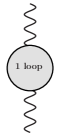
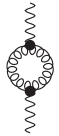
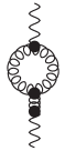
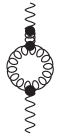
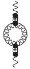
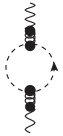
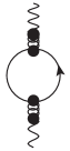
Figure 5: Diagrams contributing to the one-loop reggeized gluon self-energy.

Keeping the ${\cal O}(\rho,\rho^{0})$ terms, for $\rho\to\infty$, we have the following result:

$$\parbox{28.45274pt}{\includegraphics[width=28.45274pt]{self_1loop.pdf}}=\Sigma^{(1)}\left(\rho;\epsilon,\frac{{\bm{q}}^{2}}{\mu^{2}}\right)=\frac{(-2i{\bm{q}}^{2})\alpha_{s}N_{c}\Gamma^{2}(1+\epsilon)}{4\pi\Gamma(1+2\epsilon)}\left(\frac{{\bm{q}}^{2}}{\mu^{2}}\right)^{\epsilon}$$

$$\hskip 54.06006pt\times\bigg{\{}\frac{i\pi-2\rho}{\epsilon}-\frac{1}{(1+2\epsilon)\epsilon}\bigg{[}\frac{5+3\epsilon}{3+2\epsilon}-\frac{n_{f}}{N_{c}}\left(\frac{2+2\epsilon}{3+2\epsilon}\right)\bigg{]}\bigg{\}}.$$ (39)

It contains both finite $\sim\rho^{0}$ and divergent terms $\sim\rho$, where the latter are found to be proportional to the one-loop gluon Regge trajectory. The one-loop corrections to the quark-quark-reggeized gluon vertex $i\mathcal{M}^{(1)}_{qr^{*}\to q}$ are on the other hand obtained from evaluating the set of diagrams shown in Fig. 6.

= + + + + + +

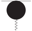
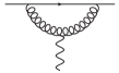
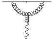
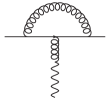
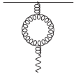
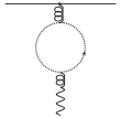
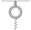
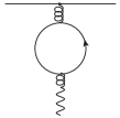
Figure 6: Contributions to the unsubtracted one-loop quark-quark-reggeized gluon vertex.

We obtain the following result

$$={i\mathcal{M}^{(0)}_{qr^{*}\to q}}\frac{\alpha_{s}N_{c}}{4\pi\epsilon}\frac{\Gamma(1+\epsilon)^{2}}{\Gamma(1+2\epsilon)}\left(\frac{{\bm{k}}^{2}}{\mu^{2}}\right)^{\epsilon}\bigg{[}-\left(\ln\frac{-p_{a}^{+}}{\sqrt{{\bm{k}}^{2}}}+\ln\frac{p_{a}^{+}}{\sqrt{{\bm{k}}^{2}}}+{\rho}\right)$$

$$+\frac{3+2\epsilon}{N_{c}^{2}2\epsilon(1+2\epsilon)}-\frac{11+7\epsilon}{(3+2\epsilon)(1+2\epsilon)}+\frac{n_{f}}{N_{c}}\frac{2+2\epsilon}{(3+2\epsilon)(1+2\epsilon)}$$

$$+\frac{2+11\epsilon}{2\epsilon(1+2\epsilon)}-\bigg{(}\psi(1-\epsilon)-2\psi(\epsilon)+\psi(1)\bigg{)}\bigg{]},$$ (40)

where $\psi(z)={\Gamma^{\prime}(z)}/{\Gamma(z)}$. In analogy with our treatment of the real NLO corrections we subtract from the above result the non-local contributions stemming from the one-loop corrections to the reggeized gluon propagator combined with the tree-level quark-reggeized gluon coupling:

$$\mathcal{C}^{(1)}_{qr^{*}\to q}\left(p_{a}^{+},\rho;\epsilon\frac{{\bm{q}}^{2}}{\mu^{2}}\right)=\parbox{56.9055pt}{\includegraphics[width=56.9055pt]{impacoeff.pdf}}=\parbox{56.9055pt}{\includegraphics[width=56.9055pt]{impaamp.pdf}}-\parbox{56.9055pt}{\includegraphics[width=56.9055pt]{impa_traj.pdf}}$$

$$=i\mathcal{M}^{(0)}_{qr^{*}\to q}\frac{\alpha_{s}}{4\pi}\left(\frac{{\bm{k}}^{2}}{\mu^{2}}\right)^{\epsilon}\frac{\Gamma^{2}(1+\epsilon)}{\Gamma(1+2\epsilon)}\left\{\frac{-2N_{c}}{\epsilon}\left(\ln\frac{p_{a}^{+}}{\sqrt{{\bm{k}}^{2}}}-\frac{\rho}{2}\right)\right.$$

$$+\left.\frac{N_{c}(2+7\epsilon)}{2\epsilon^{2}(1+2\epsilon)}+\frac{1}{N_{c}}\left(\frac{1}{\epsilon^{2}(1+2\epsilon)}+\frac{1}{2\epsilon}\right)-N_{c}\frac{1}{\epsilon}\bigg{(}\psi(1-\epsilon)-2\psi(\epsilon)+\psi(1)\bigg{)}\right\}.$$ (41)

The four-point elastic amplitude is the sum of two contributions as the one calculated above:

$$i\mathcal{M}_{q_{a}q_{b}\to q_{1}q_{2}}^{(1)}=\parbox{56.9055pt}{\includegraphics[width=56.9055pt]{qq_amp.pdf}} =\parbox{56.9055pt}{\includegraphics[width=56.9055pt]{qq_amp_traj.pdf}}+\parbox{56.9055pt}{\includegraphics[width=56.9055pt]{qq_amp_i1.pdf}}+\parbox{56.9055pt}{\includegraphics[width=56.9055pt]{qq_amp_i2.pdf}}.$$ (42)

While each of the three diagrams at the right hand side of Eq. (42) is divergent in the $\rho\to\infty$ limit, these $\rho$-divergences cancel in the sum, yielding the following result:

$$\frac{i\mathcal{M}_{q_{a}q_{b}\to q_{1}q_{2}}^{(1)}}{i\mathcal{M}_{q_{a}q_{b}\to q_{1}q_{2}}^{(0)}} =\frac{1}{2}\left(\ln\frac{s}{{\bm{k}}^{2}}+\ln\frac{-s}{{\bm{k}}^{2}}\right)\omega^{(1)}\left(\epsilon,\frac{{\bm{q}}^{2}}{\mu^{2}}\right)+\Gamma_{a}^{(1)}\left(\epsilon,\frac{{\bm{q}}^{2}}{\mu^{2}}\right)+\Gamma_{b}^{(1)}\left(\epsilon,\frac{{\bm{q}}^{2}}{\mu^{2}}\right).$$ (43)

Here the one-loop gluon Regge trajectory reads

$$\omega^{(1)}\left(\epsilon,\frac{{\bm{q}}^{2}}{\mu^{2}}\right) =-\frac{\alpha_{s}N_{c}}{2\pi\epsilon}\left(\frac{{\bm{k}}^{2}}{\mu^{2}}\right)^{\epsilon}\frac{\Gamma^{2}(1+\epsilon)}{\Gamma(1+2\epsilon)}.$$ (44)

This piece is associated to the reggeized gluon exchange, whereas

$$\Gamma^{(1)}_{a,b}\left(\epsilon,\frac{{\bm{q}}^{2}}{\mu^{2}}\right) =\frac{\alpha_{s}}{2}\left(\frac{{\bm{k}}^{2}}{\mu^{2}}\right)^{\epsilon}\bigg{[}\frac{N_{c}}{\pi}\frac{85+9\pi^{2}}{36}-\frac{\beta_{0}}{4\pi\epsilon}-\frac{5}{18}\frac{n_{f}}{\pi}$$

$$\qquad\qquad\qquad\qquad-\frac{C_{F}}{\pi}\left(\frac{1}{\epsilon^{2}}-\frac{3}{2\epsilon}+4-\frac{\pi^{2}}{6}\right)\bigg{]}+\mathcal{O}(\epsilon),$$ (45)

provides the virtual corrections to the quark impact factor. This result is in perfect agreement with the QCD calculations by [16], confirmed in [17]. At this point we would like to stress that in order to arrive at this result it is necessary to subtract in Eq. (3.3) not only the divergent pieces $\sim\rho$ but also finite terms. This is in contrast with the real contributions, where the entire central corrections are proportional to the high energy divergence. We now discuss the calculation of the gluon Regge trajectory in terms of the quark contributions.

4 Quark contribution to the NLO gluon Regge trajectory

It is useful to approach the calculation of the gluon Regge trajectory from the point of view of renormalized effective vertices and propagators. Formally, this can be understood as a renormalization of the coefficients of the reggeized gluon action as obtained after integrating out gluon and quark fields with the subsequent subtraction of non-local contributions. At the amplitude level this corresponds to the following definition of the renormalized quark-reggeized gluon coupling coefficients:

$$\mathcal{C}^{\text{R}}_{qr^{*}\to q}\left(\frac{p_{a}^{+}}{M^{+}};\epsilon,\frac{{\bm{q}}^{2}}{\mu^{2}}\right) =Z^{+}\left(\frac{M^{+}}{\sqrt{{\bm{k}}^{2}}},\rho;\epsilon,\frac{{\bm{k}}^{2}}{\mu^{2}}\right)\mathcal{C}_{qr^{*}\to q}\left(\frac{p_{a}^{+}}{\sqrt{{\bm{k}}^{2}}},\rho;\epsilon\frac{{\bm{k}}^{2}}{\mu^{2}}\right),$$ (46)

$$\mathcal{C}^{\text{R}}_{qr^{*}\to q}\left(\frac{p_{b}^{-}}{M^{-}};\epsilon,\frac{{\bm{k}}^{2}}{\mu^{2}}\right) =Z^{-}\left(\frac{M^{-}}{\sqrt{{\bm{k}}^{2}}},\rho;\epsilon,\frac{{\bm{k}}^{2}}{\mu^{2}}\right)\mathcal{C}_{qr^{*}\to q}\left(\frac{p_{b}^{-}}{\sqrt{{\bm{k}}^{2}}},\rho;\epsilon\frac{{\bm{k}}^{2}}{\mu^{2}}\right),$$ (47)

and the renormalized reggeized gluon propagator:

$$G^{\text{R}}\left(M^{+},M^{-};\epsilon,{\bm{k}}^{2},\mu^{2}\right) =\frac{G\left(\rho;\epsilon,{\bm{k}}^{2},\mu^{2}\right)}{Z^{+}\left(\frac{M^{+}}{\sqrt{{\bm{k}}^{2}}},\rho;\epsilon,\frac{{\bm{k}}^{2}}{\mu^{2}}\right)Z^{-}\left(\frac{M^{-}}{\sqrt{{\bm{k}}^{2}}},\rho;\epsilon,\frac{{\bm{k}}^{2}}{\mu^{2}}\right)},$$ (48)

with the bare reggeized gluon propagator given by

$$G\left(\rho;\epsilon,{\bm{k}}^{2},\mu^{2}\right) =\frac{i/2}{{\bm{k}}^{2}}\left\{1+\frac{i/2}{{\bm{k}}^{2}}\Sigma\left(\rho;\epsilon,\frac{{\bm{k}}^{2}}{\mu^{2}}\right)+\left[\frac{i/2}{{\bm{k}}^{2}}\Sigma\left(\rho;\epsilon,\frac{{\bm{k}}^{2}}{\mu^{2}}\right)\right]^{2}+\ldots\right\}.$$ (49)

The renormalization factors $Z^{\pm}$ cancel for the complete quark-quark scattering amplitude and can be parameterized as follows

$$Z^{\pm}\left(\frac{M^{\pm}}{\sqrt{{\bm{k}}^{2}}},\rho;\epsilon,\frac{{\bm{k}}^{2}}{\mu^{2}}\right) =\exp\left[\left(\rho-\ln\frac{M^{\pm}}{\sqrt{\bm{k}}^{2}}\right)\omega\left(\epsilon,\frac{{\bm{k}}^{2}}{\mu^{2}}\right)+f\left(\epsilon,\frac{{\bm{k}}^{2}}{\mu^{2}}\right)\right]$$ (50)

where the gluon Regge trajectory has the following perturbative expansion,

$$\omega\left(\epsilon,\frac{{\bm{k}}^{2}}{\mu^{2}}\right) =\omega^{(1)}\left(\epsilon,\frac{{\bm{k}}^{2}}{\mu^{2}}\right)+\omega^{(2)}\left(\epsilon,\frac{{\bm{k}}^{2}}{\mu^{2}}\right)+\ldots,$$ (51)

with the one-loop expression given in Eq. (44). The function $f(\epsilon,{\bm{k}}^{2})$ parametrizes finite contributions and is, in principle, arbitrary. Regge theory suggests to fix it in such a way that at one loop the non-$\rho$-enhanced contributions of the one-loop reggeized gluon self energy are entirely transferred to the quark-reggeized gluon couplings leading to

$$f^{(1)}\left(\epsilon,\frac{{\bm{k}}^{2}}{\mu^{2}}\right) =\frac{\alpha_{s}N_{c}\Gamma^{2}(1+\epsilon)}{4\pi\Gamma(1+2\epsilon)}\left(\frac{{\bm{q}}^{2}}{\mu^{2}}\right)^{\epsilon}\frac{(-1)}{(1+2\epsilon)2\epsilon}\bigg{[}2+\frac{5+3\epsilon}{3+2\epsilon}-\frac{n_{f}}{N_{c}}\left(\frac{2+2\epsilon}{3+2\epsilon}\right)\bigg{]}.$$ (52)

Using $M^{+}=p_{a}^{+}$, $M^{-}=p_{b}^{-}$ we can see that this choice for $f$ keeps the full $s$-dependence of the amplitude inside the reggeized gluon exchange, while the renormalized quark-reggeized gluon couplings agree with Eq. (3.3).

= + + + + + + + + + + + + +

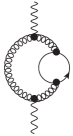
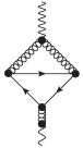
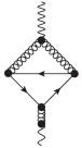
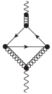
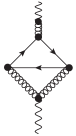
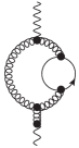
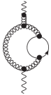
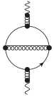
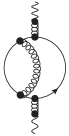
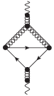
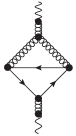
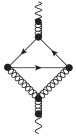
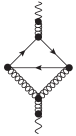
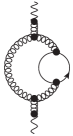
Figure 7: Diagrams contributing to the one-loop reggeized gluon self-energy.

In [8] this formalism has been put to test through the determination of the quark contributions to the two-loop gluon Regge trajectory. The complete set of contributing diagrams is given in Fig. 7. The diagrams in the second line of this figure can be neglected since they do not give $\rho$-enhanced contributions. These subleading diagrams are obtained as projections of the quark contribution to the two-loop gluon polarization tensor and are therefore finite when $\rho\to\infty$.

Among all the remaining diagrams we found that only the first one in Fig. 7 is $\rho$-enhanced. This graph is unique since the reggeized gluon couples from above and below to the usual gluon loop through an induced vertex. The complete set of enhanced contributions in Fig. 7 is given by

$$=-\rho(-i2{\bm{k}}^{2})\bar{g}^{4}\frac{4n_{f}}{\epsilon N_{c}}\frac{\Gamma^{2}(2+\epsilon)}{\Gamma(4+2\epsilon)}\cdot\frac{3\Gamma(1-2\epsilon)\Gamma(1+\epsilon)\Gamma(1+2\epsilon)}{\Gamma^{2}(1-\epsilon)\Gamma(1+3\epsilon)\epsilon}.$$ (53)

As for the one-loop corrections to the quark-quark-reggeized gluon vertex, it is needed to subtract from this result the corresponding diagrams with a reggeized gluon exchange. For the complete two-loop trajectory we have

$$\parbox{56.9055pt}{\centering\includegraphics[height=71.13188pt]{self_2loop.pdf}\@add@centering}=\parbox{56.9055pt}{\centering\includegraphics[height=71.13188pt]{self_2loop_ME.pdf}\@add@centering}-\parbox{56.9055pt}{\centering\includegraphics[height=71.13188pt]{self2_1loop.pdf}\@add@centering}.$$ (54)

More precisely, the terms to be subtracted which are both proportional to $n_{f}$ and $\rho$-enhanced read

$$\left[\parbox{42.67912pt}{\centering\includegraphics[height=71.13188pt]{self2_1loop.pdf}\@add@centering}\right]_{n_{f},\,\rho} =\hskip 11.38092pt-\rho(-2i{\bm{k}}^{2})\frac{\alpha_{s}^{2}N_{c}}{(4\pi)^{2}}\left(\frac{{\bm{k}}^{2}}{\mu^{2}}\right)^{2\epsilon}\frac{8n_{f}}{\epsilon}\frac{\Gamma^{2}(2+\epsilon)}{\Gamma(4+2\epsilon)}\frac{\Gamma^{2}(1+\epsilon)}{\Gamma(1+2\epsilon)}\frac{2}{\epsilon}.$$ (55)

The final subtracted reggeized gluon self energy, in terms of $n_{f}$ and $\rho$ contributions is

$$\Sigma^{(2)}_{n_{f}}\left(\rho;\epsilon,\frac{{\bm{k}}^{2}}{\mu^{2}}\right) =\left[\parbox{42.67912pt}{\centering\includegraphics[height=71.13188pt]{self_2loop.pdf}\@add@centering}\right]_{n_{f},\rho}=\frac{\rho(-2i{\bm{k}}^{2})\alpha_{s}^{2}N_{c}4n_{f}}{(4\pi)^{2}\epsilon}\frac{\Gamma^{2}(2+\epsilon)}{\Gamma(4+2\epsilon)}\left(\frac{{\bm{k}}^{2}}{\mu^{2}}\right)^{2\epsilon}$$

$$\qquad\qquad\qquad\times\left(\frac{\Gamma^{2}(1+\epsilon)}{\Gamma(1+2\epsilon)}\frac{4}{\epsilon}-\frac{3\Gamma(1-2\epsilon)\Gamma(1+\epsilon)\Gamma(1+2\epsilon)}{\Gamma^{2}(1-\epsilon)\Gamma(1+3\epsilon)\epsilon}\right).$$ (56)

To extract the quark contribution to the gluon Regge trajectory at two loops it is needed to identify the $\rho$-enhanced contributions of the bare reggeized gluon propagator up to two loops. These are

$$G\left(\rho;\epsilon,{\bm{k}}^{2},\mu^{2}\right) =\frac{i/2}{{\bm{k}}^{2}}\bigg{\{}1+\frac{i/2}{{\bm{k}}^{2}}\Sigma^{(1)}\left(\rho;\epsilon,\frac{{\bm{k}}^{2}}{\mu^{2}}\right)$$

$$+\frac{i/2}{{\bm{k}}^{2}}\Sigma^{(2)}\left(\rho;\epsilon,\frac{{\bm{k}}^{2}}{\mu^{2}}\right)+\left[\frac{i/2}{{\bm{k}}^{2}}\Sigma^{(1)}\left(\rho;\epsilon,\frac{{\bm{k}}^{2}}{\mu^{2}}\right)\right]^{2}+\ldots\bigg{\}}.$$ (57)

Selecting only the terms proportional to $n_{f}$, the pieces of ${\cal O}(\rho)$ in the renormalized reggeized gluon propagator at two loops are

$$G^{\text{R}}\bigg{|}_{n_{f},\rho} =\frac{i/2}{{\bm{k}}^{2}}\bigg{\{}\frac{i/2}{{\bm{k}}^{2}}\Sigma^{(2)}_{n_{f}}+\left[\frac{i/2}{{\bm{k}}^{2}}\Sigma^{(1)}\left(\rho;\epsilon,\frac{{\bm{k}}^{2}}{\mu^{2}}\right)\right]^{2}\bigg{|}_{n_{f},\rho}$$

$$\qquad\qquad-\rho\,\omega^{(1)}\left(\epsilon,\frac{{\bm{k}}^{2}}{\mu^{2}}\right)f^{(1)}_{n_{f}}\left(\epsilon,\frac{{\bm{k}}^{2}}{\mu^{2}}\right)-\rho\,\omega^{(2)}_{n_{f}}\left(\epsilon,\frac{{\bm{k}}^{2}}{\mu^{2}}\right)\bigg{\}}$$ (58)

with

$$f^{(1)}_{n_{f}}\left(\epsilon,\frac{{\bm{k}}^{2}}{\mu^{2}}\right) =n_{f}\frac{\alpha_{s}\Gamma^{2}(1+\epsilon)}{4\pi\Gamma(1+2\epsilon)}\left(\frac{{\bm{q}}^{2}}{\mu^{2}}\right)^{\epsilon}\bigg{(}\frac{2+2\epsilon}{3+2\epsilon}\bigg{)}$$ (59)

being the part proportional to $n_{f}$ of $f^{(1)}$ in Eq. (52). The requirement that the $\rho$ dependence in Eq. (4) has to cancel in the limit $\rho\to\infty$ then yields the quark contribution to the gluon Regge trajectory at two loops as

$$\omega^{({2})}_{n_{f}}\left(\epsilon,\frac{{\bm{k}}^{2}}{\mu^{2}}\right) =\frac{\alpha_{s}^{2}N_{c}}{4\pi^{2}}\left(\frac{{\bm{k}}^{2}}{\mu^{2}}\right)^{2\epsilon}\frac{n_{f}}{\epsilon}\frac{\Gamma^{2}(2+\epsilon)}{\Gamma(4+2\epsilon)}$$

$$\qquad\times\bigg{[}\frac{\Gamma^{2}(1+\epsilon)}{\Gamma(1+2\epsilon)}\frac{2}{\epsilon}-\frac{3\Gamma(1-2\epsilon)\Gamma(1+\epsilon)\Gamma(1+2\epsilon)}{\Gamma^{2}(1-\epsilon)\Gamma(1+3\epsilon)\epsilon}\bigg{]},$$ (60)

which is in perfect agreement with Eq.(9) of the original study of Fadin et al. in [18]. This confirms the validity of our approach to the effective action at two loop level and the regularization prescription here presented.

5 Conclusions and Outlook

In these contribution a brief introduction to Lipatov’s effective action to describe high energy processes in QCD has been given. This effective action is not obtained through a reduction of the number of degrees of freedom, but rather adds a new degree of freedom through the reggeized gluon. This leads to a series of subtleties that have been recently addressed in [9, 8, 19] by means of a regularization and subtraction procedure that ensures the locality in rapidity. Several non-trivial checks of the validity of this prescription, including one- and two-loop computations, have been performed finding agreement with previous results in the literature. We have explicitly discussed the quark-initiated forward jet vertex and quark contributions to the gluon Regge trajectories at next-to-leading order. The gluon-initiated jet vertex and the gluon contributions to the gluon trajectory will be presented elsewhere [19].

References

- [1] L. N. Lipatov, Sov. J. Nucl. Phys. 23 (1976) 338, E. A. Kuraev, L. N. Lipatov, V. S. Fadin, Phys. Lett. B 60 (1975) 50, Sov. Phys. JETP 44 (1976) 443, Sov. Phys. JETP 45 (1977) 199; I. I. Balitsky, L. N. Lipatov, Sov. J. Nucl. Phys. 28 (1978) 822.
- [2] V. Fadin, L. Lipatov, Phys. Lett. B 429 (1998) 127; M. Ciafaloni, G. Camici, Phys. Lett. B 430 (1998) 349.
- [3] M. Deak, F. Hautmann, H. Jung and K. Kutak, JHEP 0909 (2009) 121 [arXiv:0908.0538 [hep-ph]], arXiv:1012.6037 [hep-ph], Eur. Phys. J. C 72 (2012) 1982 [arXiv:1112.6354 [hep-ph]], G. Chachamis, M. Hentschinski, A. Sabio Vera and C. Salas, arXiv:0911.2662 [hep-ph], D. Colferai, F. Schwennsen, L. Szymanowski and S. Wallon, JHEP 1012 (2010) 026 [arXiv:1002.1365 [hep-ph]], M. Angioni, G. Chachamis, J. D. Madrigal and A. Sabio Vera, Phys. Rev. Lett. 107 (2011) 191601 [arXiv:1106.6172 [hep-th]], F. Hautmann, M. Hentschinski and H. Jung, Nucl. Phys. B 865 (2012) 54 [arXiv:1205.1759 [hep-ph]], arXiv:1205.6358 [hep-ph], M. Hentschinski, A. Sabio Vera and C. Salas, arXiv:1209.1353 [hep-ph], A. van Hameren, P. Kotko and K. Kutak, arXiv:1211.0961 [hep-ph].
- [4] L. N. Lipatov, Nucl. Phys. B452 (1995) 369-400, Phys. Rept. 286 (1997) 131-198.
- [5] E.N.Antonov, L.N.Lipatov, E.A.Kuraev, I.O.Cherednikov, Nucl. Phys. B721 (2005) 111-135.
- [6] M. Hentschinski, Acta Phys. Polon. B39 (2008) 2567-2570; arXiv:0908.2576 [hep-ph]; Nucl. Phys. Proc. Suppl. 198 (2010) 108-111. M. Hentschinski, J. Bartels, L. N. Lipatov, [arXiv:0809.4146 [hep-ph]].
- [7] M. A. Braun, M. Y. .Salykin, S. S. Pozdnyakov and M. I. Vyazovsky, arXiv:1209.2490 [hep-ph], M. A. Braun, L. N. Lipatov, M. Y. .Salykin and M. I. Vyazovsky, Eur. Phys. J. C 71 (2011) 1639 [arXiv:1103.3618 [hep-ph]], M. A. Braun and M. I. Vyazovsky, Eur. Phys. J. C 51 (2007) 103 [hep-ph/0612323].
- [8] G. Chachamis, M. Hentschinski, J. D. Madrigal Martinez and A. Sabio Vera, Nucl. Phys. B 861 (2012) 133 [arXiv:1202.0649 [hep-ph]].
- [9] M. Hentschinski and A. Sabio Vera, Phys. Rev. D 85 (2012) 056006 [arXiv:1110.6741 [hep-ph]].
- [10] V. N. Gribov, “The theory of complex angular momenta: Gribov lectures on theoretical physics,” Cambridge, UK: Univ. Pr. (2003) 297 p
- [11] H. Weigert, Prog. Part. Nucl. Phys. 55 (2005) 461 [hep-ph/0501087].
- [12] I. Balitsky, Nucl. Phys. B 463 (1996) 99 [hep-ph/9509348].
- [13] A. van Hameren, P. Kotko and K. Kutak, arXiv:1207.3332 [hep-ph].
- [14] M. Ciafaloni and D. Colferai, Nucl. Phys. B 538 (1999) 187 [hep-ph/9806350].
- [15] M. Hentschinski, Nucl. Phys. B 859 (2012) 129 [arXiv:1112.4509 [hep-ph]].
- [16] V. S. Fadin, R. Fiore and A. Quartarolo, Phys. Rev. D 50 (1994) 2265 [hep-ph/9310252].
- [17] V. Del Duca and C. R. Schmidt, Phys. Rev. D 57 (1998) 4069 [hep-ph/9711309].
- [18] V. S. Fadin, R. Fiore and M. I. Kotsky, Phys. Lett. B 387 (1996) 593 [hep-ph/9605357].
- [19] G. Chachamis, M. Hentschinski, J. D. Madrigal Martinez and A. Sabio Vera, in preparation.